Decoding Cerebrospinal Fluid: Integrative Metabolomics Across Multiple Platforms
Antoine Presset, Sylvie Bodard, Antoine Lefèvre, Edward Oujagir, Camille Dupuy, Jean-Michel Escoffre, Lydie Nadal-Desbarats

TL;DR
This paper introduces a standardized method to study cerebrospinal fluid using multiple technologies to better understand brain chemistry.
Contribution
A new integrative multiplatform metabolomic workflow combining 1H-NMRS and HPLC-MS for CSF analysis is introduced.
Findings
Integrating 1H-NMRS and HPLC-MS improves metabolite coverage in CSF.
The workflow enables reliable characterization of the CSF metabolome.
The method supports discovery of potential CNS biomarkers.
Abstract
Cerebrospinal fluid (CSF) is a key biological matrix that reflects the physiological and pathological states of the central nervous system (CNS). It supports brain function by regulating ionic balance, facilitating molecular transport, and clearing metabolic waste. In this article, we present a standardized protocol for CSF collection along with an integrative multiplatform metabolomic workflow that combines proton nuclear magnetic resonance spectroscopy (1H-NMRS) and high-performance liquid chromatography coupled to mass spectrometry (HPLC-MS). Integrating these complementary analytical modalities enhances metabolite coverage and improves analytical robustness, enabling a more comprehensive and reliable characterization of the CSF metabolome. This workflow supports the discovery of potential biomarkers and advances our understanding of neurochemical alterations within the CNS.
Genes, proteins, chemicals, diseases, species, mutations and cell lines named across the full text — each resolved to its canonical identifier and authoritative record.
Click any figure to enlarge with its caption.
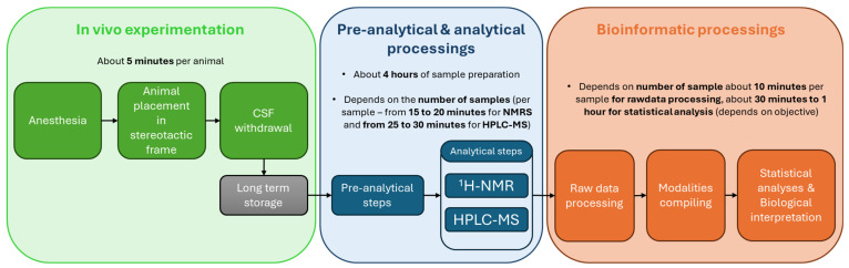 Figure 1
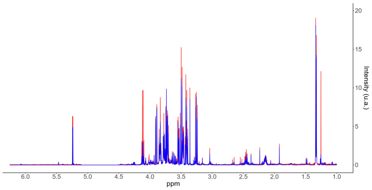 Figure 2
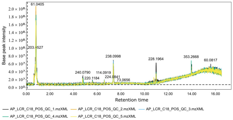 Figure 3
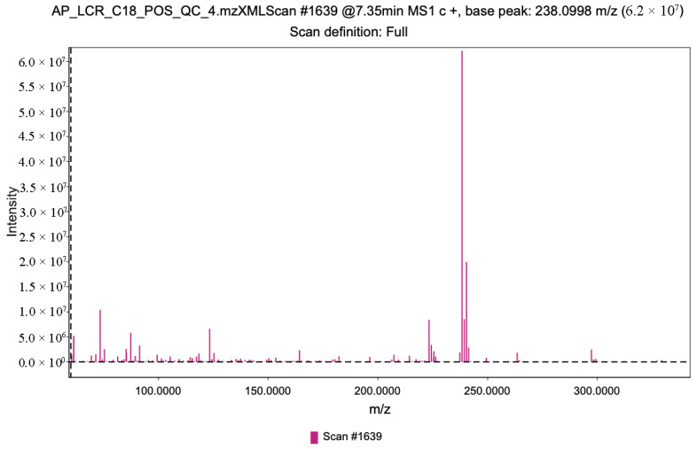 Figure 4
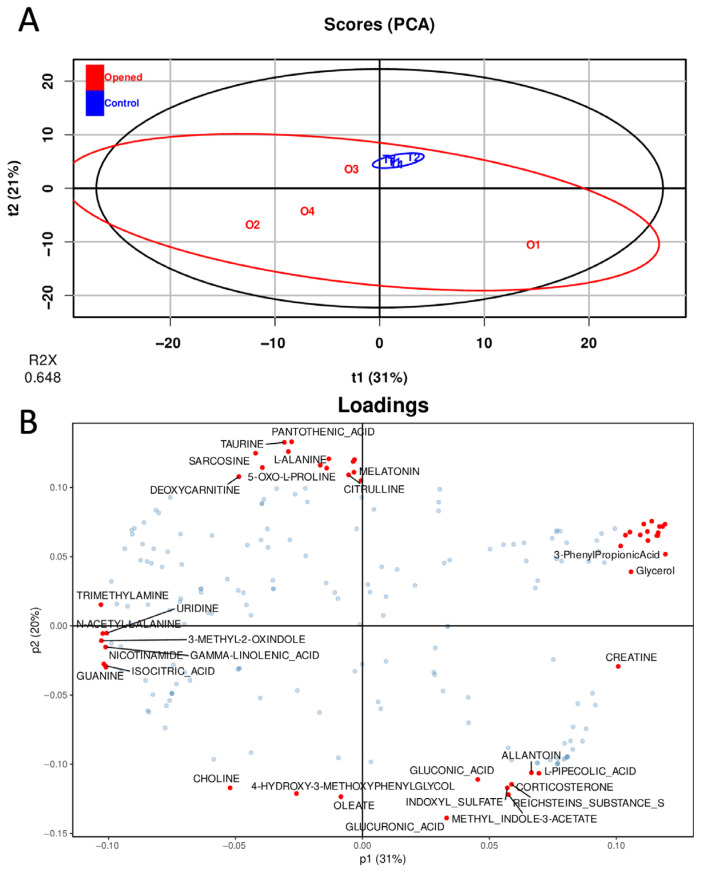 Figure 5
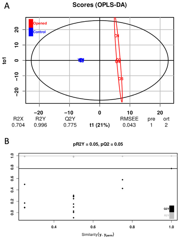 Figure 6
 Figure 7
- —UMR 1253
- —iBraiN
- —Université de Tours, Inserm
- —la Ligue Contre le Cancer
- —Agence Nationale de la Recherche
Peer Reviews
No public reviews on file for this paper yet. If you reviewed it on a platform where reviews are public (OpenReview, ICLR, NeurIPS, ICML), you can paste yours below so the community can read it here.
Videos
No videos yet. Explain this paper in a talk, walkthrough, or lecture? Add one.
Taxonomy
TopicsMetabolomics and Mass Spectrometry Studies · Neuroscience and Neuropharmacology Research · Cerebrospinal fluid and hydrocephalus
1. Introduction
The meninges are three protective membranes surrounding the brain and spinal cord: the dura mater, arachnoid membrane, and pia mater [1,2]. Cerebrospinal fluid (CSF) is a clear, colorless liquid located within the ventricles and subarachnoid spaces. In adult humans, the total CSF volume is approximately 150 mL (about 25 mL within the ventricles and 125 mL in the subarachnoid spaces). CSF is primarily secreted by the choroid plexuses in the ventricles, although the brain interstitial fluid, the ependyma, and cerebral capillaries also contribute to its composition [3]. CSF circulation is mainly driven by the arterial pulse wave, but respiration, posture, venous pressure, and physical activity also influence its flow and pressure dynamics [4]. CSF provides hydromechanical protection, regulates interstitial fluid composition, modulates neuronal activity, and plays a central role in maintaining cerebral homeostasis by clearing metabolic waste and regulating ionic balance [5]. Alterations in CSF dynamics or composition can therefore disrupt brain function [6]. The choroid plexus, located in the lateral, third, and fourth ventricles, is the principal site of CSF secretion. This vascularized structure is composed of choroidal epithelial cells, ependymal cells, endothelial cells, connective stroma, and a rich capillary network [7]. Choroidal epithelial cells, characterized by apical microvilli and tight junctions, actively transport ions and water to produce CSF. Ependymal cells, lining the ventricles and continuous with choroidal epithelium, contribute to regulating CSF volume and composition. Endothelial cells mediate exchanges between blood and CSF compartments [3,7]. CSF secretion involves (1) passive filtration of plasma into the choroidal interstitial space; (2) active ion transport across the choroidal epithelium via cytoplasmic carbonic anhydrase and ion carriers; (3) intracellular conversion of CO_2_ and H_2_O into H^+^ and HCO_3_^−^ by carbonic anhydrase; and (4) exchange of these ions for Na^+^ and Cl^−^ at the basolateral membrane. ATP-dependent pumps on the apical membrane subsequently transport Na^+^, Cl^−^, HCO_3_^−^, and K^+^ into the ventricular lumen, followed by osmotic water movement through aquaporin I channels [8]. Disturbances in CSF production, circulation, or absorption can lead to significant CSF dysfunctions, including hydrocephalus, intracranial pressure dysregulation, or infection [9]. As a result, CSF analysis is a critical tool for evaluating CNS disorders, enabling the detection of metabolic abnormalities and the identification of potential biomarkers.
Metabolomics—the systematic study of small molecules (metabolites) within a biological system—aims to identify and quantify these compounds to capture the organism’s functional state. Unlike genomics or proteomics, metabolomics provides a direct snapshot of the metabolic phenotype, reflecting the combined effects of the genetic, environmental, and biochemical factors [10]. This field primarily relies on mass spectrometry (MS) and nuclear magnetic resonance (NMR) spectroscopy, used either in targeted (specific metabolites) or untargeted (global profile) approaches depending on study objectives [11]. To the best of our knowledge, only a limited number of studies have employed an integrative NMR- and Liquid-Chromatography MS-based metabolomics approach in rats, regardless of the biological matrices analyzed, even though such integrative strategies leverage the complementary strengths of each technique. NMR enables the direct and non-invasive identification of metabolites, offering a substantial advantage for both qualitative and quantitative analysis. However, its sensitivity is often insufficient for detecting low-abundance metabolites. In contrast, Liquid Chromatography coupled to mass spectrometry (LC-MS) provides high sensitivity and can analyze a broad spectrum of metabolites with remarkable precision, although it typically requires more complex sample preparation and does not always offer the same level of direct structural identification as NMR. Recently Kim et al. (2023) reported an ex vivo NMR-based metabolomics approach using cerebrospinal fluid for the diagnosis of primary CNS lymphoma, correlating metabolic signatures with MR imaging features. Their findings suggest that while NMR metabolomics may aid in diagnosing primary central nervous system lymphoma (PCNSL), it is less informative for the prognosis [12]. To further strengthen such metabolomics investigations, one could envision that combining NMR and LC-MS would provide a more comprehensive characterization of metabolic alterations. Similarly, Locasale et al. (2012) studied changes in CSF constituents using high-throughput LC-MS/MS analysis in a small cohort of patients with malignant glioma compared with control subjects [13]. Using targeted MS-based metabolomics and unsupervised statistical techniques, they identified metabolic signatures, mainly involving polar metabolites (tryptophan’s derivative and citric acid cycle components), that distinguished glioma patients from controls. Additionally, Nielsen et al. (2021) characterized Alzheimer’s disease (AD) using an integrative NMR- and LC-MS-based metabolomics workflow. By combining these two methodologies, they identified multiple altered pathways related to AD pathology [14]. Current challenges in this field notably include the complexity of integrating datasets generated from these fundamentally different analytical platforms. Here, we describe a complete protocol for CSF collection in rats before and after a transient blood–brain barrier opening (BBBO) induced by microbubble-assisted ultrasound, coupled with a comprehensive multiplatform metabolomics workflow integrating ^1^H-NMR spectroscopy and HPLC-MS.
2. Experimental Design
CSF is collected from anesthetized animals positioned in a stereotaxic frame using only ear bars. This method is adapted from Ceaglio et al. and Pegg et al. [15,16]. A maximum of 200 µL of CSF can be collected per rat. Samples are immediately placed on ice and centrifuged, and the supernatant is transferred to sterile Eppendorf tubes for storage at −80 °C. For downstream analyses, each CSF sample is aliquoted into three tubes corresponding to the different analytical modalities by the two platforms. Metabolite extraction procedures are adapted to each modality (i.e., ^1^H-NMR and HPLC-MS using a C18 column or HPLC-MS using an HILIC column), including a protein precipitation step using methanol (MeOH). During this pre-analytical step, quality control (QC) samples—either pooled study samples or reference materials—are used in metabolomics workflows to monitor and evaluate the variability and reliability of analytical platforms throughout the entire experiment. QC samples ensure data consistency, enable the detection of technical variability, and help identify potential systematic errors during sample acquisition. To assess analytical performance, several QCs should be injected at the beginning and the end of each analytical run, as well as after every ten samples (depending on the total sample set). Preparing QCs requires calculating the appropriate pooling volume from each individual sample and processing the pooled aliquots in the same manner as all study samples. Our protocol primarily targets polar metabolites to generate a rapid and representative snapshot of the metabolome (e.g., amino acids, carbohydrates, tricarboxylic acids, etc.). Metabolite identification and quantification are achieved using the ASICS R package (R version 4.5.2—ASICS package version 2.24.0) for NMR spectra and the XCalibur software (version 2.2) for HPLC-MS data. Results are exported as tables of relative metabolite intensities or abundancies. Finally, statistical analyses—multivariate, univariate, and pathway integration—are conducted to interpret metabolomic profiles (Figure 1).
2.1. Materials
Kinetex XB C18 (Phenomenex Incorporation; Torrance, CA, USA).Cortecs HILIC (Waters Corporation; Milford, MA, USA).Mass Spectroscopy Metabolite Library of Standards (IROA Technologies, Sea Girt, NJ, USA).25G sterile winged infusion set (SV*25NL30; Terumo, Tokyo, Japan).1 mL sterile syringe (MDSS01SE; Terumo, Tokyo, Japan).500 µL sterile Eppendorf tubes.Ethanol (EtOH) 70% (v/v).Betadine.Electric shaver.Stereotaxic frame.Anesthetic (ketamine/xylazine or isoflurane).Acetonitrile, HPLC-MS grade.Methanol (MeOH), HPLC-MS grade.MilliQ water (18.2 MΩ.cm at 25 °C, TOC 3 ppb, <1 particle/mL).Trimethylsilyl propionate (TSP).
2.2. Equipment
Stereotaxic frame model 963 (Kopf Instruments; Tujunga, CA, USA).Ultra High-Performance Liquid Chromatography (UPLC) Ultimate WPS-3000 (Dionex; Sunnyvale, CA, USA).Q-Exactive hybrid quadrupole-Orbitrap mass spectrometer (Thermo Fisher Scientific; Bremen, Germany).DRX-600 Avance III HD NMR spectrometer with Triple Resonance Inverse Cryoprobe (Bruker; Billerica, MA, USA).
3. Procedure
3.1. CSF Withdrawal
CRITICAL STEP At least two experimenters are required—one to operate the syringe and the other to stabilize the winged needle.
- Anesthetize the animal using a ketamine/xylazine mixture (70 mg/kg and 7 mg/kg, respectively). Alternative approved anesthetic methods may also be used.
- Place it in the stereotaxic frame with only ear bars.
- Tilt the head downward at a 15° to 20° angle relative to the vertical axis to expose the foramen magnum at the C1 vertebra (atlas).
- Secure the head with the tooth bar.
- Shave, depilate, and clean the neck with 70% ethanol followed by betadine.
- Identify the puncture site at the intersection of two lines: one connecting the external occipital protuberance to the spinal column and the other joining the two mastoid processes.
- Apply gentle negative pressure by slightly pulling the syringe plunger during insertion.
- Position the winged needle at a 90° angle relative to the horizontal plane of the skin surface at the sampling site. Ensure that the orientation of the wings is parallel to the ear bars.
- Collect a maximum of 200 µL of CSF. This is the maximum volume recommended prior to sacrifice to avoid physiological disturbance.
CRITICAL STEP If any red blood cells (RBCs) enter the winged needle tubing, the second experimenter must immediately clamp and then cut the tube. Cutting the tube without prior clamping may generate suction, which could draw additional RBCs into the system.
- 10.Immediately place the collected CSF on ice.
- 11.Centrifuge the sample at 10,000× g for 15 min at 4 °C to remove any cellular debris.
- 12.Transfer the supernatant to a clean, sterile Eppendorf tube.
- 13.Store the processed CSF samples at −80 °C until further analysis.
3.2. Pre-Analytical Procedure
CRITICAL STEP Aliquot each sample into two 50 µL tubes and one 100 µL tube for the three different analytical modalities. Include quality control (QC) samples to assess analytical platform variation: several QC samples should be analyzed at the beginning and end of each run and after every 10 samples.
3.2.1. HPLC-MS
Pipette 50 µL of each sample into a clean microcentrifuge tube.Add 300 µL of cold methanol (–20 °C).Vortex for 5 s to ensure proper mixing.Incubate at −20 °C for 30 min to precipitate proteins.Centrifuge at 5000× g for 25 min at 4 °C.Carefully collect a fixed volume of supernatant (e.g., 250 µL), ensuring that the pellet remains undisturbed.Transfer to new tubes and evaporate to dryness using a vacuum concentrator (35 °C, 3 h).Reconstitute dried extracts for the following:
- a.HILIC column: 100 µL of acetonitrile/water (9:1, v/v).
- b.C18 column: 100 µL of methanol/water (1:9, v/v). Vortex briefly to dissolve completely.Transfer reconstituted samples to HPLC vials for injection and analysis.
3.2.2. 1H-NMR
Dilute the CSF sample 1:4 by cold methanol (–20 °C) to a final volume of 200 µL.Vortex briefly.Centrifuge at 4000× g for 10 min at 4 °C to pellet precipitated proteins.Transfer a fixed volume of supernatant (e.g., 80 µL) into a clean hemolysis tube.Dry under vacuum using a SpeedVac (35 °C, 2 h).Immediately before acquisition, reconstitute the dried extract in 200 µL of phosphate buffer (prepared in D_2_O) with 10 µL of 3.2 mM of TSP as a chemical shift reference (leading to a 152 μM final concentration in the NMR tube).Vortex gently to ensure full dissolution.Transfer to NMR tube and proceed with data acquisition.
3.3. Analytical Procedure
CRITICAL STEP Preparation steps may vary depending on the equipment used. All samples must be analyzed simultaneously on the same analytical platform to ensure comparability. Three aliquots were prepared: the first for C18 HPLC-MS, the second for HILIC HPLC-MS, and the third for NMR analysis. For HPLC-MS experiments, it is essential to first construct a commercial reference library as described in the Reference Library Construction Section.
3.3.1. HPLC-MS
Chromatographic Column Setup
C18 Column Conditions
Set up the UPLC Ultimate WPS-3000 system equipped with a Kinetex XB C18 (150 mm × 2.1 mm, 1.7 µm) under the following conditions:
- Column temperature: 55 °C.
- Mobile phase A: Milli-Q water with 0.1% (v/v) formic acid.
- Mobile phase B: Methanol with 0.1% (v/v) formic acid.
- Flow rate: 0.2 mL/min.
- Gradient duration: 28 min for both positive and negative ionization modes. Run analyses by injecting samples into a mass spectrometer configured as described in the Mass Spectrometer Analysis Section.
HILIC Column Conditions:
Prepare a UPLC Ultimate WPS-3000 system equipped with a Cortecs HILIC (150 mm × 2.1 mm, 1.6 µm) under the following conditions:
- Column temperature: 55 °C.
- Mobile phase A: Milli-Q water with 10 mM of ammonium formate.
- Mobile phase B: Acetonitrile with 10 mM of ammonium formate.
- Flow rate: 0.2 mL/min.
- Gradient duration: 22 min for positive ionization mode. Run analyses by injecting samples into a mass spectrometer configured as described below.
Mass Spectrometer Analysis
Configure the Q-Exactive hybrid quadrupole-Orbitrap mass spectrometer for both positive and negative electrospray ionization (ESI) mode as follows:
- Spray voltage: ±3000 V.
- Capillary temperature: 325 °C.
- Heater temperature: 350 °C.
- Sheath gas flow: 25 arbitrary units (AU).
- Auxiliary gas flow: 8 AU.
- Sweep gas flow: 3 AU.
- S-Lens RF level: ±100 V. Configure the analyzer and the detector as follows:
- Acquisition mode: Full scan.
- Mass range: 58–870 m/z.
- Resolution: 70,000 at m/z 200.
- AGC target: 1 × 10^6^ charges.
- Maximum injection time: 250 ms.
CRITICAL STEP QC samples must be injected at the beginning and end of the run and after every 10 samples to monitor analytical stability.
3.Inject samples in the analytical platforms.
- a. Injection volume:
- A total of 5 µL for C18 column.
- A total of 10 µL for HILIC column.
3.3.2. 1H-NMR
CRITICAL STEP As for HPLC-MS, QC samples should be analyzed first and last in the sequence, and after every 10 samples, to ensure data quality and reproducibility.
- Place each NMR tube in a rack and insert the rack into the sample changer of the Bruker DRX-600 Avance III HD spectrometer (Bruker, Billerica, MA, USA).
- The probe must be tuned to the proper frequency to detect the signal of ^1^H.
- Lock the magnetic field on the deuterium resonance from the solvent used (here, D_2_O + H_2_O), followed by shimming to optimize field homogeneity.
- Set up the acquisition parameters: pulse sequence with water suppression, 90° pulse, sweep width, relaxation delay, number of dummy scans, number of scans, and time domain.
- Start the NMR acquisition.
3.4. Data Processing
3.4.1. HPLC-MS
Reference Library Construction
Use the Mass Spectroscopy Metabolite Library of Standards (IROA Technologies, Sea Girt, NJ, USA), containing 610 standard metabolites, to build an in-house spectral reference library.Analyze these standards under the same chromatographical and mass spectrometry conditions as the biological samples (as described in Section 3.3.1).
Metabolite Identification
Identify metabolites in biological samples by matching spectral features against the in-house reference library.Verify by using the XCalibur 2.2 software (Thermo Fisher Scientific, San Jose, CA, USA) for metabolite identification according to the following four criteria:
- Retention time must be within ±20 s of the standard.
- Measured mass must be within ±10 ppm of the theoretical mass.
- Peak shape and isotopic distribution must be consistent with the reference spectrum of the standard.
- Metabolites exhibiting a relative standard deviation greater than 30% are excluded from the final dataset. Metabolites with a signal-to-noise ratio (SNR) < 3 are discarded.
Peak Integration and Intensity Extraction
For metabolites meeting all four identification criteria, integrate the area under the corresponding chromatographic peak to determine intensity.Export results as a data matrix containing metabolite identifiers and their intensities across all samples.
3.4.2. 1H-NMR
Free Induction Decay (FID) Processing
The obtained FID signal is converted into a spectrum by applying a Fourier transformation using TopSpin 3.6.2 (Bruker, Billerica, MA, USA).Apply zero filling and exponential multiplication with a line broadening of 0.3 Hz.Apply zero- and first-order phase correction.Perform baseline flattening and align spectral peaks if necessary.Normalize the spectra using the internal reference compound (TSP or another molecule).
Metabolite Identification and Quantification
Identify and quantify spectral peaks by deconvoluting and reconstructing NMR spectra using a library of pure compounds implemented in the ASICS R package [17,18].Run the ASICS workflow to quantify a maximum of 190 metabolites.Export results as a data table containing relative quantifications across all samples.
3.4.3. Quality Control and Database Attributes
CRITICAL STEP All data matrices must be organized with metabolites as rows and samples as columns. QC samples must be analyzed concurrently with study samples.
Calculate the coefficient of variation (CV) of each metabolite within QC samples for all analytical platforms (C18 ESI+, C18 ESI-, HILIC+, and NMR) as follows:
Remove all metabolites showing a CV greater than 30%.Using metabolite databases (in-house database, KEGG, Reactome, HMDB, etc.), associate each metabolite to a unique identifier (e.g., glucose → KEGG ID: C00031).Save curated data matrices for redundancy filtering.
3.5. Statistical Analysis
3.5.1. Redundancy Filtering and Normalization
Compile a unified data table containing metabolites from each analytical modality and tag them with their corresponding modality (C18 ESI+, C18 ESI-, HILIC+, and NMR).For metabolites detected by multiple platforms, retain the measure from the modality showing the lowest CV in the QC samples.Remove QC samples from the data matrix and normalize CSF samples to the total ion or spectral area [19,20,21].
3.5.2. Multivariate Analyses
Perform multivariate analyses using R and the ropls package (version 1.40.0) [22] or equivalent statistical software.
- a.Unsupervised analysis: perform a Principal Component Analysis (PCA) to explore clustering and detect potential outliers.
- b.Supervised analysis: perform a Partial Least Squares Discriminant Analysis (PLS-DA) to identify group discriminants. Assess model performance using Q^2^, where values closer to 1 indicate stronger predictive ability.Validate model significance through permutation testing (implemented in ropls), ensuring pR^2^Y and pQ^2^ are <0.05 and Q^2^ is >0.5.Identify significant metabolites based on Variable Importance in Projection (VIP) scores. Select those with a VIP > 1 for further analyses.
OPTIONAL STEP Receiver Operating Characteristic (ROC) curves may be plotted to evaluate the predictive performance of discriminant metabolites, either individually or in combination [23]. The area under the curve (AUC) indicates the ability to correctly classify new samples.
3.5.3. Univariate Analyses
Assess data normality using the Shapiro–Wilk test and homogeneity of variances using the Fligner–Killeen test.Choose the appropriate statistical test (parametric or non-parametric) depending on these results to identify metabolites differing significantly between groups.Adjust p-values for multiple testing using the Bonferroni correction [24] or other suitable methods.Metabolites are considered significantly altered when the adjusted p-value is < 0.05.Calculate the log_2_ Fold Change (Log2 FC) for all significantly different metabolites.
OPTIONAL STEP A volcano plot can be used to visualize metabolites according to their log_2_ fold change and statistical significance (−log_10_ p-value). Metabolites with a Log2 FC > 1 and a −log_10_ p-value > 1.30 were selected as candidates for further investigation.
3.5.4. Biological Integration
Identify metabolites showing significant differences between experimental groups or use metabolites with a VIP > 1 and a |Log2 FC| > 1.Determine affected metabolic pathways using KEGG identifiers and perform Over-Representation Analysis (ORA) via a hypergeometric test, which evaluates whether certain metabolites are statistically over-represented in a pathway.A pathway is considered significantly impacted when the adjusted p is <0.05.Manually inspect significantly dysregulated pathways and remove non-relevant ones (i.e., pathways containing metabolites without reaction biochemical relationships).
4. Expected Results
This section describes the raw and processed data obtained from a multiplatform CSF metabolomics study. A metabolomics workflow generates large and complex datasets: a three-dimensional dataset for HPLC-MS (intensity, retention time, and mass-to-charge ratio) and a two-dimensional dataset (intensity and chemical shift) for NMR spectroscopy. After data processing, metabolite identification and quantification yield structured tables. Because each analytical platform offers complementary yet sometimes overlapping information, redundancy filtering is required. Some metabolites are detectable on only one platform, while others are shared across several. Given the high dimensionality of the data (many metabolites, samples, and experimental conditions), multivariate statistical approaches are preferred. Unsupervised methods (e.g., PCA) enable exploration of inherent data structure, while supervised methods (e.g., PLS-DA or OPLS-DA) identify discriminant metabolites associated with experimental groups. Healthy Sprague–Dawley rats (Janvier Labs, Le Genest-Saint-Isle, France) were housed in an animal facility under a 12 h/12 h light/dark cycle with ad libitum access to food and water. Upon arrival, the rats were 7 weeks old. After a mandatory one-week acclimation period, their average body weight was 340 g (±12 g). Animals were randomly assigned to groups of four per cage. This workflow was applied to eight 2-month-old rats subjected to transient BBBO using microbubble-assisted ultrasound: four control animals and four animals sampled 3 h post-BBBO. This procedure consisted of transiently opening the BBB through the combined action of an intravenous injection of microbubbles and their activation by ultrasound generated by a probe positioned above the skull. Animals were placed in a stereotaxic frame, the skull was exposed, and bregma was used as a reference point to position the ultrasound transducer over the right striatum (anteroposterior: −0.5 mm; laterality: −3.15 mm; depth: 5 mm). A volume of 100 µL of microbubbles was injected via the caudal vein, followed by 100 µL of saline to flush the line. The target region was then exposed to 1 MHz ultrasound for 30 s using a pulse repetition frequency (PRF) of 1 Hz and 10,000 cycles per pulse, corresponding to a burst length (BL) of 10 ms, to transiently open the BBB. CSF was subsequently collected from anesthetized animals positioned in a stereotaxic frame using only ear bars. As this procedure was terminal, animals were euthanized after CSF sampling by administering a lethal dose corresponding to three times the anesthetic induction dose. All CSF withdrawals were successful, and no animal died during the collection procedure.
Raw NMR spectra undergo Fourier transformation followed by post-processing steps—phase and baseline correction—to enhance spectral quality and quantification accuracy (Figure 2). After processing, spectral peaks are identified and quantified using the ASICS R package, which reconstructs spectra based on a reference library of pure compounds [17,18]. This workflow quantifies up to 190 metabolites, producing a data table of relative metabolite intensities (or concentrations if normalized to TSP) across samples.
Each retention time corresponds to a series of scans capturing ion fragments related to a given metabolite (Figure 3). Each chromatographic peak is associated with a specific mass-to-charge (m/z) value (Figure 4). Together, retention time (RT) and m/z pairs constitute the fundamental identifiers used for metabolite annotation.
Table 1 provides an overview of the metabolites detected and quantified in the CSF prior to redundancy filtering (Table 1). Approximately 50% of the redundancy was removed using the CV threshold criterion.
In Table 2, creatine appears across all four analytical modalities, illustrating redundancy in the dataset. To address this, the CV calculated from QC samples is used to determine which modality provides the highest reproducibility and, therefore, the most reliable signal across platforms. HPLC-MS C18 ESI^+^ modality exhibited the lowest CV and was consequently retained in the final matrix. KEGG identifiers are then added to facilitate downstream biological interpretation.
Each individual sample is represented in the scores plot based on the first two principal components, with each point labeled according to its sample name (Figure 5A). The first and second components capture 31% and 21% of the total variance, respectively, explaining 52% of the variability in the dataset. The distribution of samples forms an ellipse reflecting the inter-individual heterogeneity within the overall metabolic pattern. PCA analysis reveals a clear and compact clustering of control animals, whereas rats subjected to transient BBBO exhibit a more dispersed distribution, indicating greater inter-individual variability in their metabolic response. The loadings plot (Figure 5B) illustrates the variables contributing to the principal components. While the scores plot displays the sample positions in the PCA space, the loading plot identifies the metabolites driving those positions. Variables located farther from the origin have stronger contributions to the components, and the angles between their vectors represent correlations (close alignment indicates a positive correlation, while the opposite orientation indicates a negative correlation). In this study, the loading plot provides a global view of the variables underlying the observed clustering. Further discrimination between groups can be obtained using supervised methods, such as OPLS-DA (Figure 6), which infer class membership based on experimental groups.
OPLS-DA is a supervised multivariate statistical method used to model differences between predefined groups. In contrast to PCA, which is unsupervised and captures only the directions of maximum variance within the dataset, OPLS-DA partitions the variation into two components: (i) predictive variation, which is correlated with group membership, and (ii) orthogonal variation, which is unrelated to group differences. This separation enhances model interpretability and facilitates the identification of variables (e.g., metabolites) that drive class discrimination. In an OPLS-DA score plot, groups appear clearly separated because the method explicitly optimizes discrimination, underscoring the need for rigorous model validation to avoid misinterpretation or overfitting. A permutation test is therefore required to verify that the observed separation reflects a true biological difference rather than chance. The procedure involves repeatedly permuting group labels (typically 100–1000 permutations); rebuilding the OPLS-DA model for each permutation; and recalculating performance metrics, such as R^2^ and Q^2^. The metrics of the original model are then compared with the distribution of permuted metrics using a statistical test. If the original model’s R^2^ and Q^2^ are significantly higher (with pR2Y and pQ2 representing p-values), the model is considered robust and unlikely to reflect random structure. In our study, the OPLS-DA model achieved a Q^2^Y value of 0.775, exceeding the commonly accepted threshold of 0.5 and indicating strong predictive performance (Figure 6A). The permutation test confirmed the validity of the model (pR^2^Y = 0.05; pQ^2^ = 0.05) (Figure 6B). Variable Importance in Projection (VIP) scores were used to quantify each metabolite’s contribution to the class separation; metabolites with a VIP > 1 were considered discriminant. Eighty-six metabolites met this criterion and were subsequently subjected to univariate analysis using the non-parametric Dunn test with Bonferroni correction. After statistical filtering, 26 metabolites were significantly different between the two experimental groups. Table 3 presents the top 10 discriminant metabolites with their log_2_ fold-change values and adjusted p-values (Table 3), while all significant metabolites are listed in Appendix A (Table A1).
Biological interpretation of metabolomics data relies on pathway analysis, which situates metabolites within metabolic networks to explain phenotypes. These analyses use curated databases, such as KEGG, HMDB, and Reactome [25,26,27]. Using the KEGG database, a hypergeometric test was performed as part of ORA (Table 4) [28]. This test evaluates the probability that a set of metabolites is statistically over-represented within a pathway. Raw p-values are adjusted using the False Discovery Rate (FDR) correction, with significance set at an adjusted p-value of <0.05.
Only the arginine biosynthesis pathway reached statistical significance after FDR correction (p = 4.44 × 10^−4^; FDR = 0.035). Alanine, aspartate, and glutamate metabolism (p = 3.60 × 10^−3^; FDR = 0.144) and tryptophan metabolism (p = 0.010; FDR = 0.284) exhibited the lowest raw p-values, suggesting potential enrichment trends (Table 4) as the FDR values did not reach significance. A complete table can be found in (Appendix A—Table A2). These preliminary findings indicate that arginine and related amino-acid pathways may be affected. Arginine plays a key role in reducing reactive oxygen and nitrogen species, supporting energy metabolism, regulating vascular tone, and modulating immune functions [29,30,31]. This versatile amino acid participates in numerous biological processes and can be converted into proline and glutamate [29]. Through its metabolic pathways, arginine contributes to protein synthesis, nitric oxide (NO) production, creatine synthesis, and polyamine biosynthesis—processes essential for cell growth, proliferation, and differentiation. It also supports nitrogen detoxification via the urea cycle. Because endothelial cells are the first targets of microbubble-assisted ultrasound [32], arginine is readily used by endothelial arginase, directing its metabolism towards the urea cycle, polyamine formation and the synthesis of proline or glutamate from ornithine. Arginine is also catabolized by nitric oxide synthase (NOS) to generate NO and citrulline, a reaction requiring cofactors, such as NADPH, FMN, FAD, and tetrahydrobiopterin. As the precursor of NO, arginine contributes to vasodilation, angiogenesis, and immune cytotoxicity [33]. Moreover, arginine availability influences macrophage polarization toward M1 or M2 phenotypes [31]. Analysis of CSF metabolism indicates that acoustically mediated BBBO disrupts arginine metabolism. These findings suggest that the procedure alters metabolic processes within the endothelial cells. Further investigation of arginine metabolism is therefore warranted, including mechanistic analyses of the pathways involved. Increasing the number of animals or developing approaches enabling repeated CSF sampling over time would help refine these conclusions. Our multiplatform analytical workflow is optimized for the discovery and quantification of polar metabolites in central metabolic pathways (e.g., amino-acid and carbohydrate metabolisms). However, protein precipitation with cold methanol does not efficiently extract apolar metabolites, such as lipids. Although lipids remain present in the sample, excessive lipid content can contaminate the NMR spectral signal and distort the baseline. CSF is naturally rich in phospholipids, glycerolipids, cerebrosides, ceramides, lysolipids, and related lipid classes [34,35,36]. Implementing a biphasic extraction protocol (e.g., Matyash MTBE, Bligh–Dyer, or Folch) would therefore be valuable to incorporate a lipidomic dimension into the analysis.
5. Reagent Setup
Phosphate Buffer Preparation: dissolve K_2_HPO_4_ and KH_2_PO_4_ in D_2_O to reach pH 7.4.
TSP Solution: prepare TSP solution in D_2_O at a final concentration of 3.2 mM.
The reference list from the paper itself. Each links out to its DOI / PubMed record.
- 1Sakka L. Coll G. Chazal J. Anatomy and physiology of cerebrospinal fluid Eur. Ann. Otorhinolaryngol. Head Neck Dis.201112830931610.1016/j.anorl.2011.03.00222100360 · doi ↗ · pubmed ↗
- 2Sakka L. Chazal J. The meninges, an anatomical point of view Morphologie 200589354210.1016/S 1286-0115(05)83236-915943079 · doi ↗ · pubmed ↗
- 3Reiber H. Proteins in cerebrospinal fluid and blood: Barriers, CSF flow rate and source-related dynamics Restor. Neurol. Neurosci.200321799610.3233/RNN-2003-0022914530572 · doi ↗ · pubmed ↗
- 4Zervas N.T. Liszczak T.M. Mayberg M.R. Black P.M. Cerebrospinal fluid may nourish cerebral vessels through pathways in the adventitia that may be analogous to systemic vasa vasorum J. Neurosurg.19825647548110.3171/jns.1982.56.4.04757062119 · doi ↗ · pubmed ↗
- 5Pollay M. The function and structure of the cerebrospinal fluid outflow system Cerebrospinal Fluid Res.20107910.1186/1743-8454-7-920565964 PMC 2904716 · doi ↗ · pubmed ↗
- 6Ayub M. Jin H.K.J. Bae J. The blood cerebrospinal fluid barrier orchestrates immunosurveillance, immunoprotection, and immunopathology in the central nervous system BMB Rep. Korean Soc. Biochem. Mol. Biol.20215419620210.5483/BMB Rep.2021.54.4.205PMC 809394133298242 · doi ↗ · pubmed ↗
- 7Engelhardt B. Sorokin L. The blood–brain and the blood–cerebrospinal fluid barriers: Function and dysfunction Semin. Immunopathol.20093149751110.1007/s 00281-009-0177-019779720 · doi ↗ · pubmed ↗
- 8Owler B.K. Pitham T. Wang D. Aquaporins: Relevance to cerebrospinal fluid physiology and therapeutic potential in hydrocephalus Cerebrospinal Fluid Res.201071510.1186/1743-8454-7-1520860832 PMC 2949735 · doi ↗ · pubmed ↗