Enhanced HoVerNet Optimization for Precise Nuclei Segmentation in Diffuse Large B-Cell Lymphoma
Gei Ki Tang, Chee Chin Lim, Faezahtul Arbaeyah Hussain, Qi Wei Oung, Aidy Irman Yajid, Sumayyah Mohammad Azmi, Yen Fook Chong

TL;DR
This paper improves HoVerNet for precise nuclei segmentation in DLBCL, a common lymphoma, using deep learning and a user-friendly tool to aid diagnosis.
Contribution
The study optimizes HoVerNet for CMYC-stained images and integrates it into a GUI for real-time diagnostic support in DLBCL.
Findings
HoVerNet achieved 82.5% validation accuracy with strong precision and recall in nuclei segmentation.
The GUI enhanced efficiency and usability for DLBCL histopathological analysis.
The model effectively managed overlapping and complex nuclei morphology.
Abstract
Background/Objectives: Diffuse Large B-Cell Lymphoma (DLBCL) is the most common subtype of non-Hodgkin lymphoma and demands precise segmentation and classification of nuclei for effective diagnosis and disease severity assessment. This study aims to evaluate the performance of HoVerNet, a deep learning model, for nuclei segmentation and classification in CMYC-stained whole slide images and to assess its integration into a user-friendly diagnostic tool. Methods: A dataset of 122 CMYC-stained whole slide images (WSIs) was used. Pre-processing steps, including stain normalization and patch extraction, were applied to improve input consistency. HoVerNet, a multi-branch neural network, was used for both nuclei segmentation and classification, particularly focusing on its ability to manage overlapping nuclei and complex morphological variations. Model performance was validated using metrics…
Genes, proteins, chemicals, diseases, species, mutations and cell lines named across the full text — each resolved to its canonical identifier and authoritative record.
Click any figure to enlarge with its caption.
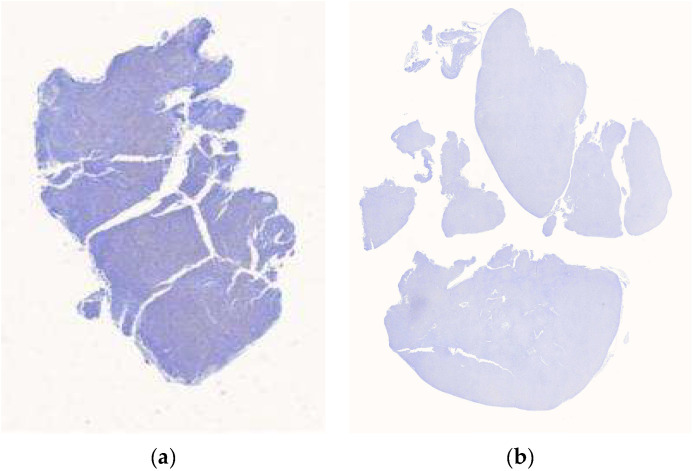 Figure 1
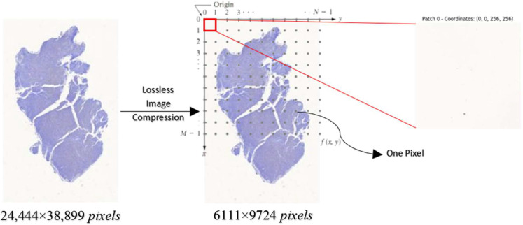 Figure 2
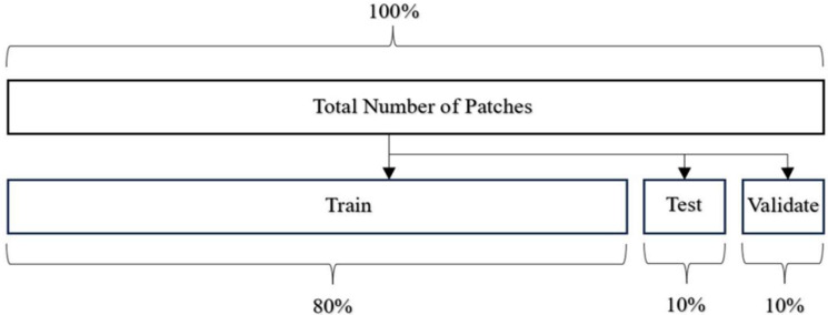 Figure 3
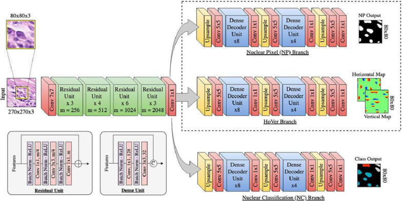 Figure 4
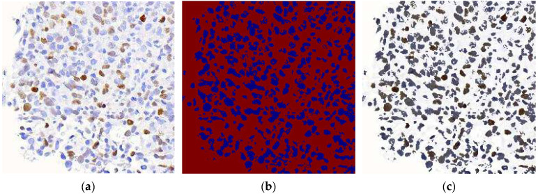 Figure 5
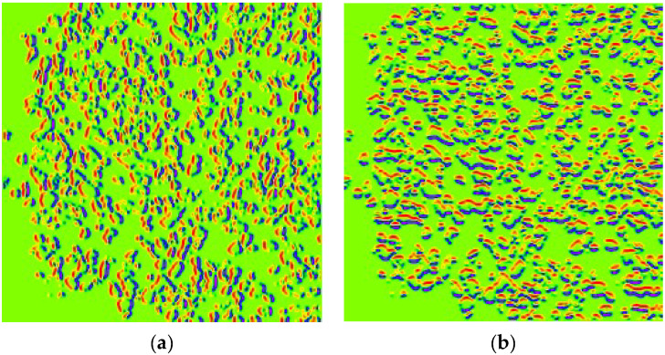 Figure 6
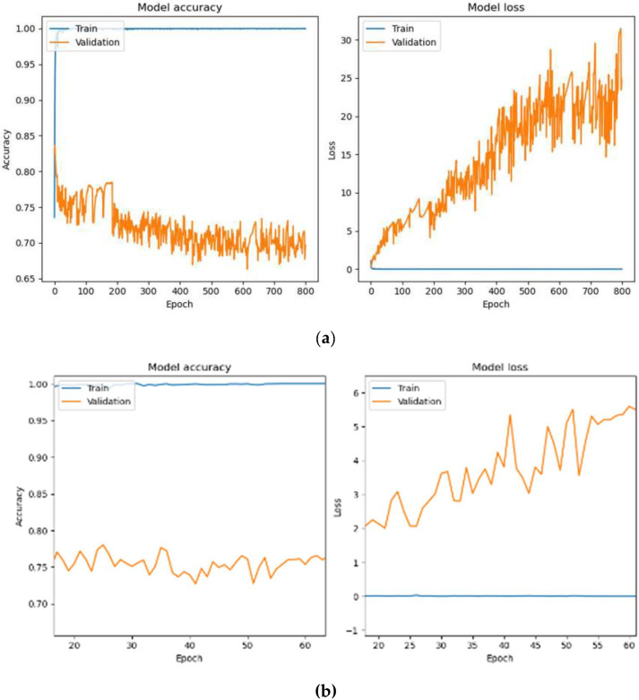 Figure 7
 Figure 8
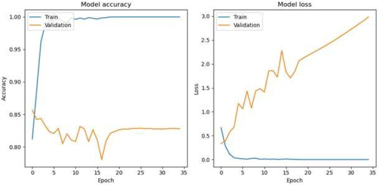 Figure 9
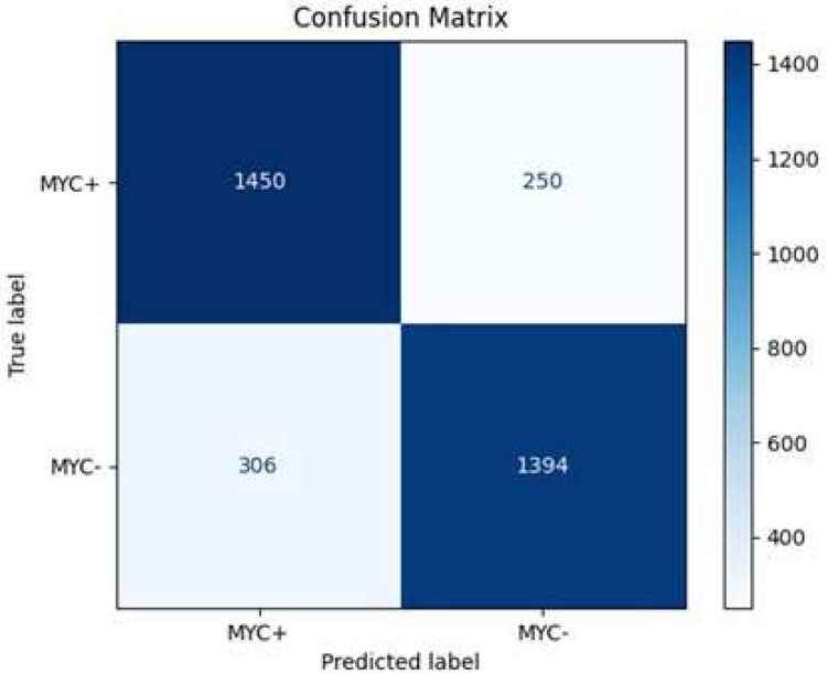 Figure 10
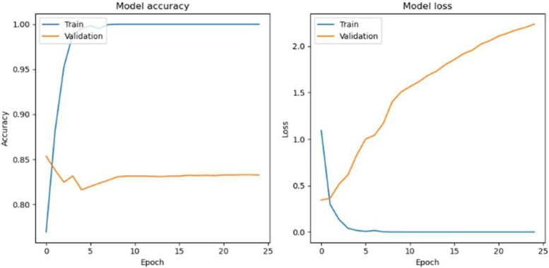 Figure 11
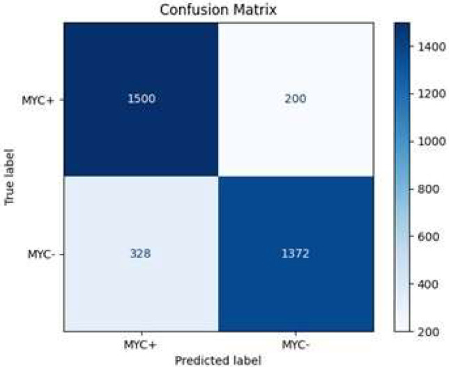 Figure 12
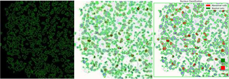 Figure 13
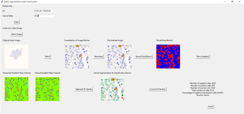 Figure 14
- —Ministry of Higher Education (MoHE), Malaysia, through the Fundamental Research Grant Scheme (FRGS)
- —Universiti Sains Malaysia
Peer Reviews
No public reviews on file for this paper yet. If you reviewed it on a platform where reviews are public (OpenReview, ICLR, NeurIPS, ICML), you can paste yours below so the community can read it here.
Videos
No videos yet. Explain this paper in a talk, walkthrough, or lecture? Add one.
Taxonomy
TopicsAI in cancer detection · Radiomics and Machine Learning in Medical Imaging · Digital Imaging for Blood Diseases
1. Introduction
Accurate segmentation and classification of nuclei are crucial in the analysis of Diffuse Large B-Cell Lymphoma (DLBCL) tissue images [1]. Proper identification and quantification of tumor cells can significantly impact diagnosis and treatment planning. Traditional methods of nuclei segmentation and classification often struggle with challenges such as tissue heterogeneity, staining variability, and complex cellular interactions, leading to slow, labor-intensive processes prone to errors. These challenges highlight the need for more efficient, automated approaches to enhance diagnostic accuracy.
Deep learning, particularly convolutional neural networks (CNNs), has revolutionized the field of medical image analysis. CNNs are proficient at learning intricate patterns from data, making them highly effective in segmenting and classifying nuclei, even under difficult conditions. These networks excel in extracting relevant features such as nucleus shape, size, and texture, enabling accurate tissue analysis. However, while CNNs have shown great promise, existing techniques still face limitations in handling complex cases, such as overlapping nuclei and varying tissue morphologies, especially in diseases like DLBCL.
HoVerNet, an advanced deep learning architecture, offers a promising solution to these challenges. This method employs multi-branch processing to perform both segmentation and classification simultaneously, making it highly effective for the analysis of clustered, heterogeneous nuclei. HoVerNet’s ability to extract precise morphological features, such as nuclear area, perimeter, and shape, allows for more accurate tumor cell quantification. It also opens the door to the development of new prognostic markers and improvements in diagnostic accuracy, addressing the gaps left by traditional methods.
This research aims to leverage HoVerNet’s capabilities to enhance the diagnosis, subtyping, and severity assessment of DLBCL. By addressing the current limitations in medical imaging techniques, this approach promises to improve the precision and efficiency of DLBCL analysis, aiding pathologists in making better-informed clinical decisions. The innovation lies in combining deep learning with tissue image analysis to create a more automated, accurate, and clinically useful framework for cancer diagnosis.
2. Literature Review
Image patches are small, square regions extracted from larger medical images for tasks such as region of interest (ROI) identification, feature extraction, and AI algorithm applications. They enhance analysis by focusing on specific areas, such as structures and textures, with patch sizes varying from single pixels to predefined windows. Basu et al. [2] captured 500 DLBCL and non-DLBCL tissue images at 40× magnification using microscope-based cameras, while El Hussien et al. [3] analyzed 256 × 256 patches from digitally stained H&E slides of CLL, aCLL, and RT cases. Wójcik et al. [4] standardized 37,665 H&E images of DLBCL lymph nodes to 448 × 448 pixels, and Li et al. [5] captured 400× magnification images from 500 labeled DLBCL tissue sections. Swiderska-Chadaj et al. [6] digitized 42 H&E DLBCL slides for external validation, and Bándi et al. [7] extracted annotated patches from six tissue types using WSIs. Shankar et al. [8] analyzed classic Hodgkin lymphoma, mantle cell lymphoma, and DLBCL cores at 40× magnification, while Swiderska-Chadaj et al. [9] derived 512 × 512 patches at 5× magnification for training. Perry et al. [10] applied a self-supervised phase on FFPE H&E-stained biopsy WSIs of aggressive B-cell lymphoma, dividing 20× or 40× images into 384 × 384 patches for analysis.
Pre-processing prepares image data for model input, reducing training time and improving inference. Techniques include orientation, resizing, grayscale conversion, and exposure adjustments to enhance image quality and feature extraction. Hamdi et al. [11] applied Gaussian filters, Laplacian filters, color normalization, and Gradient Vector Flow for feature extraction. Vrabac et al. [12] used tissue microarrays for cell nucleus extraction from H&E-stained images, while Basu et al. [2] developed attention map transformers and feature fusion for DLBCL classification. Blanc-Durand et al. [13] employed resampling, padding, cropping, and adaptive thresholding on PET and CT data to extract tumor heterogeneity features. Ferrández et al. [14] used Gaussian filtering, metabolic tumor volume, and standard uptake value metrics to analyze tumor dissemination. El Hussien et al. [3] annotated ROIs and measured nuclear contour and hull areas, while Graham et al. [15] applied Otsu thresholding, color adjustments, and textural feature extraction. Ferrández et al. [16] and Mohlman et al. [17] utilized normalization, filtering, max-pooling, ReLU operations, and edge detection in pre-processing workflows. Other studies [8,9,10,18,19,20,21] applied normalization, machine learning algorithms, filtering, and feature selection for enhanced image quality and accurate DLBCL classification.
Deep learning, especially CNNs, is highly effective in processing and classifying medical images, such as distinguishing healthy and cancerous cells in DLBCL. HoVerNet excels in nuclei segmentation and classification by integrating segmentation and classification branches, leveraging nuclear pixel distances, and enabling complex pathology analysis. Vrabac et al. [12], El Hussein et al. [3], Wójcik et al. [4], and Graham et al. [15] applied or trained HoVerNet for various tasks, with training epochs ranging from 50 to 800. Hamdi et al. [11] achieved superior performance using MobileNet-VGG-16 with an AUC of 99.43% and 99.8% accuracy on 15,000 H&E-stained WSIs. Blanc-Durand et al. [13] and Ferrández et al. [14,16] utilized 3D U-Net with Adam optimization for PET/CT scans, while Swiderska-Chadaj et al. [6] and Bándi et al. [7] also employed U-Net. Additionally, Basu et al. [2] and Vrabac et al. [12] used DenseNet-201 and ResNet-50, respectively, with optimized training parameters for DLBCL analysis. A study evaluating 17 CNN models (including VGG16) across three hospitals reported average patch-level diagnostic accuracy between 87–96%, demonstrating strong performance in DLBCL vs. non-DLBCL differentiation [5].
However, there are still challenges in nuclei segmentation and classification for DLBCL that need to be addressed. Many studies do not work well with different staining types like CMYC and H&E, which limits their use. Most research also does not focus on adding these tools into real clinical workflows or electronic medical records (EMRs), which are important for practical use. Scalability and real-time analysis are also not well explored, as many methods are not designed for large-scale use. This study helps solve these problems by showing that HoVerNet performs better on CMYC-stained images, creating a simple GUI.
3. Materials and Methods
A total of 122 digital WSIs of DLBCL, comprising 61 MYC+ cells and 61 MYC- cells, were collected from the Department of Pathology, Hospital Universiti Sains Malaysia (Hospital USM). These WSIs were scanned at 40× magnification using the Motic EasyScan Pro digital slide scanner. The collection and use of these images followed ethical guidelines outlined in the Declaration of Helsinki. Approval was obtained from the Jawatankuasa Etika Penyelidikan Manusia Universiti Sains Malaysia (JEPeM-USM), under the reference USM/JEPeM/22110749, ensuring compliance with ethical and legal standards. Only CMYC-stained images were used in this study due to the availability and standardization of these samples within the dataset. While this ensures consistency in analysis and training, it limits the model’s generalizability to other staining protocols, such as H&E. Figure 1 illustrates the examples of CMYC-stained whole slide images.
3.1. Lossless Image Compression
Lossless image compression is a type of image compression method that reduces the image file size without losing any important information [22]. The process begins by loading the image using the ‘PIL’ library [23]. The image is opened and identified using the ‘Image.open()’ function. Once the image is loaded, the next step is to resize it by using the ‘resize()’ function, which takes two parameters: the new size of the image and the resampling filter. The new size is taken by modifying the value of the resize factor, by which both width and height are divided by the resize factor. The resampling filter used is the ‘Image.LANCZOS’ function, which is known for producing high-quality results. The function is nonzero only within the interval (−1 < x < 1). After resizing, the image is saved to the specified output path using the ‘save()’ function. Lossless image compression reduces the file size of images without sacrificing important information, preserving data quality for analysis. This is achieved using the LANCZOS resampling filter, which provides high-quality results by smoothing the image while retaining sharpness and detail. This method ensures that the compressed images maintain essential features needed for segmentation and classification tasks. By resizing images, computational requirements for model training and inference are significantly reduced, enabling faster processing while retaining the integrity of nuclei features. The Lanczos function is defined as in (1).
3.2. Image Patches
Image patching is a crucial technique for localizing ROI, extracting features, reducing computational complexity, and enhancing accuracy in analyzing DLBCL images [24]. By breaking down these images into smaller patches, specific ROIs like DLBCL nuclei can be localized and analyzed. These patches allow the computation of various attributes such as color, texture, gradients, and shapes. Analyzing patches rather than the entire image reduces computational complexity, making segmentation and classification algorithms more manageable. Additionally, focusing on smaller regions allows algorithms to better handle variations in intensities, shapes, or textures, potentially leading to more accurate segmentation results. The formula for image patching is expressed as in (2). Figure 2 depicts the flow process of image patches. The original WSI, with dimensions of 24,444 × 38,899 pixels, undergoes lossless image compression, reducing its dimensions to 6111 × 9724 pixels. Following compression, the resized image is divided into square patches during the image patching process, with each patch measuring 256 × 256 pixels.
3.3. Normalization
Normalization is a crucial preprocessing step in medical image analysis, particularly for nuclei segmentation and classification. It enhances image quality, reduces distortions, and adjusts pixel intensity values to a consistent range [25], typically between 0 (black) and 1 (white). Normalization involves identifying and outlining the cell containing ROI within the image. This ensures better feature extraction by mitigating noise from lighting or staining variations. For grayscale images, normalization is applied to a single channel, while for RGB images, it is applied to all three channels. This step improves model stability, generalization, and accuracy, especially when dealing with dark, unevenly illuminated patches or datasets with diverse staining techniques. The normalization process is described as in (3).
3.4. CNN Architecture
The dataset was split into 80% training, 10% testing, and 10% validation subsets after patch extraction, not by whole slide images. This ensured a diverse and balanced distribution of input images for the CNN models. This distribution ensures sufficient data for model optimization while retaining samples for unbiased evaluation and fine-tuning (Figure 3). HoVerNet was chosen because it is specifically designed for both nuclei segmentation and classification, which is important for DLBCL analysis [4,11,15]. Its encoder-decoder structure with residual units improves feature extraction and segmentation accuracy [11]. The up-sampling branches further enhance classification by precisely predicting nucleus types, enabling the network to handle clustered and morphologically diverse nuclei in DLBCL WSIs. This study enhances the original HoVerNet framework by adapting it for CMYC-stained WSIs of DLBCL, addressing morphological and staining variations not considered in the original model. The architecture is modified for binary classification of MYC+ and MYC˗ nuclei, aligned with clinical relevance in lymphoma assessment. Model performance is optimized through systematic hyperparameter tuning, and a diagnostic scoring method based on MYC expression is introduced to estimate disease severity. Based on the literature, it performs better than U-Net and ResNet. U-Net is effective for segmentation but does not include classification, making it less suitable for identifying nucleus types [15]. ResNet is good for general image classification but lacks features needed for detailed segmentation of overlapping nuclei, which is common in DLBCL tissue images. A multi-class deep learning study using VGG16 successfully distinguished between benign nodes, DLBCL, Burkitt lymphoma, and small lymphocytic lymphoma with 95% accuracy [26]. These findings from previous studies guided the decision to use HoVerNet and to compare with VGG16 in this work. A GUI is developed to enable real-time segmentation, cell counting, and severity visualization, supporting practical integration into clinical workflows.
Figure 4 illustrates the HoVerNet architecture [11]. The model was trained for 800 epochs to ensure comprehensive learning of complex patterns in DLBCL datasets [4]. The model was implemented using PyTorch version 2.2.0, with minor modifications to support binary classification of MYC+ and MYC- nuclei. The training used the Adam optimizer with a learning rate of 1 × 10^−4^ and a batch size of 32 and 64. The binary cross-entropy loss function was applied to optimize performance for binary classification. Patch size was 256 × 256 pixels as described in Section 3.2. This choice was guided by the high complexity of the data, requiring extended training to capture intricate features [4]. Early stopping, a common technique to prevent overfitting, was considered but not implemented in this study. Instead, overfitting was managed by closely monitoring validation loss and using batch size adjustments.
3.5. Nuclei Counting and Diagnosis of Severity Level of Cells
After segmenting and classifying nuclei using HoVerNet in DLBCL images, nuclei counting is proposed. The segmented image identifies and labels each nucleus based on its type: normal cells are smaller (average 36.7 pixels), appearing dark blue; positive cancer cells are larger (average 73.5 pixels), lighter blue; negative cancer cells are also large (average 73 pixels), with a lighter blue hue. Cell counting involves using connected component labeling algorithms to distinguish and count these nucleus types. The counts are validated against manual or other automated methods. Subsequently, totals of abnormal (negative and positive) and all cells (normal, negative, and positive) are calculated. Percentages of negative and positive cells relative to total cells are then computed using a formula as in (4).
Disease severity is assessed based on nucleus characteristics like size, shape, color, and abnormalities, with each cell assigned a severity score. Cells exceeding 40% in abnormality are classified as ‘Severe’; otherwise, they are ‘Mild’. This process aids in diagnosing and monitoring disease progression in DLBCL. The 40% threshold was determined through consultation with clinical pathologists and reflects a typical cutoff observed in high-grade cases of DLBCL where MYC-positivity exceeds this level [27].
3.6. Graphic User Interface (GUI)
The data collection and preparation begin with a GUI where patient details like Patient ID and Year of Data are input to associate image analysis with the correct patient records. Once validated, the user selects an image file (PNG, JPG, JPEG, BMP, GIF) for analysis. The selected image and its patches are normalized to enhance contrast and displayed for inspection. Nuclei detection follows, converting images to grayscale if needed and applying binary thresholding for nuclei segmentation (‘Nuclei Pixel Branch’) visualized on the GUI.
Gradient computation (‘HoVer Branch’) highlights textural patterns and directional changes, aiding detailed feature analysis. Nuclei are segmented and classified based on predefined criteria, visualized to show categorization into ‘Negative Cells’, ‘Positive Cells’, and ‘Normal Cells’. Cell counting follows, tallying each type and computing total counts. The proportion of negative and positive cells is used to determine disease severity (‘Severe’ or ‘Mild’). Results, including counts, percentages, and severity assessments, are displayed on the GUI for comprehensive analysis. A ‘Finish’ button concludes analysis, confirming the completion of cell counting.
4. Results and Discussion
4.1. Image Pre-Processing
DLBCL WSIs while maintaining image quality. Using the LANCZOS filter, the resizing process preserved a resolution of 96 dpi and a bit depth of 24 bits, ensuring clarity and color fidelity. This reduction effectively minimizes computational overhead, facilitating more efficient downstream processing. Following compression, image patching yielded 34,000 distinct 256 × 256-pixel patches. Each patch was uniquely named based on its coordinates within the original image and systematically stored. Visualization of these patches revealed diverse pathological features, improving granularity for deep learning applications. This structured patch extraction enhances the deep learning model’s ability to focus on specific tissue regions within DLBCL images, optimizing feature learning for classification and analysis. Normalization of the extracted patches further improved consistency by scaling pixel intensity values to the [0,1] range, achieved through division by 255. This transformation mitigated variability in raw pixel values, leading to improved model stability and faster convergence during training. Standardization plays a crucial role in optimizing deep learning performance, ensuring more accurate and efficient analysis of DLBCL images.
4.2. Performance Evaluation of HoVerNet Optimization Results
Before feeding the images into HoVerNet and VGG16, the dataset is divided into training, testing, and validation sets (Table 1).
HoVerNet consists of three branches: the ‘Nuclei Pixel Branch,’ the ‘HoVer Branch,’ and the ‘Nuclei Classification Branch.’ The process starts with normalized patched images as input. These images are processed to detect nuclei, producing a binary image where nuclei pixels are set to one value (blue), and non-nuclei pixels are set to another value (red), as shown in Figure 5b. The output from the ‘Nuclei Pixel Branch’ is then overlaid on the normalized patched image, creating a composite image. In this overlay, the nuclei are distinctly highlighted against the background, making them easier to visually identify and analyze.
The overlay image is then projected onto the horizontal and vertical axes to create horizontal and vertical images, respectively. This process introduces an additional branch called the ‘HoVer Branch’ (Figure 6). These projections provide useful summaries of the spatial distribution of the nuclei in the image. For example, a horizontal projection provides information on how the nuclei are distributed from top to bottom, while a vertical projection provides information on how they are distributed from left to right.
After defining the architecture, an instance of the HoVerNet model was created and compiled using the Adam optimizer and binary cross-entropy loss function, suitable for binary classification tasks. The model was initially trained for 800 epochs with batch sizes of 32 and 64, following the approach of Wójcik et al. [4], who reported achieving the highest F1 score of 0.939 for similar tasks.
Figure 7a depicts the training process of the HoVerNet model over 800 epochs with a batch size of 32. The model achieved perfect training accuracy of 100% and an exceptionally low training loss of 2.21 × 10^−4^. However, validation and testing accuracy were notably lower, at 69.63% and 71.26%, with higher validation and testing losses at 24.7998 and 23.0890, respectively. These results indicate overfitting, as the model performed well on training data but failed to generalize effectively to unseen data. Figure 7b focuses on the training dynamics for a batch size of 32 over a zoomed-in epoch range of 20–60. While the training accuracy was consistently 100%, validation performance remained unstable, showing fluctuations in accuracy and higher validation losses. This pattern indicates overfitting, as the model was overly tuned to the training data and struggled to generalize to unseen data.
Figure 8a shows the training and validation performance when using a batch size of 64. The model achieved 100% training accuracy, with an even lower training loss of 1.07 × 10^−7^. Validation and testing accuracies improved to 74.68% and 75.75%, respectively, with reduced validation losses of 12.4109 and testing loss of 11.9979. The larger batch size resulted in more stable training, with fewer parameter updates per epoch, enabling better generalization to unseen data.
Figure 8b provides a closer analysis of training with a batch size of 64 between epochs 20 and 60. A sharp decline in training accuracy occurred at epoch 45 due to adjustments in model parameters to balance training and validation losses. After this drop, the training accuracy quickly recovered and stabilized at 100%. Validation accuracy showed steady improvement, and validation losses decreased over time, demonstrating the model’s ability to generalize effectively. However, after epoch 45, the accuracy of validation gradually decreases as the epoch increases. This indicates that HoVerNet achieves better performance and generalization when trained for fewer epochs (less than 45).
Further investigation into the optimal number of epochs (15, 20, 25, 30, 35, 45, and 50) aimed to maximize validation and testing accuracies while minimizing losses (Table 2). For batch size 32, the model reached 100% training accuracy by epoch 35, with validation and testing accuracy peaking at 82.78% and 83.67%, respectively. Beyond this, accuracy declined, indicating overfitting. At epoch 100, training accuracy decreased to 98.72%, with further drops in validation and testing accuracies, suggesting underfitting and potential learning rate issues.
The optimal epoch for a batch size of 32 for the HoVerNet and VGG16 models is 35 (Figure 9), where validation and testing accuracies were highest, balancing effective generalization and minimizing overfitting. This iterative approach allowed for fine-tuning the model’s training dynamics and enhancing its ability to generalize effectively. Based on the confusion matrix in Figure 10, the HoVerNet model correctly identified 1450 MYC+ instances and 1394 MYC- instances, resulting in a high true positive (TP) and true negative (TN) count. However, it misclassified 250 MYC- instances as MYC+ (FP) and 306 MYC+ instances as MYC- (FN).
Based on Table 2 and Table 4, VGG16 achieved higher classification accuracy compared to HoVerNet. However, VGG16 is a standard CNN not inherently designed for nuclei segmentation tasks. It performs well in distinguishing image-level classes but lacks the ability to accurately delineate individual nuclei, especially in cases of overlapping structures. In contrast, HoVerNet is specifically optimized for nuclear instance segmentation and classification, making it more adept at handling the complex morphological variations and overlapping nuclei commonly seen in histopathological images of DLBCL. Although its overall accuracy is lower than VGG16, HoVerNet offers superior segmentation granularity and biological interpretability, which are essential for meaningful diagnostic assessment in clinical practice.
These results are tabulated in Table 3, with an overall accuracy of approximately 85.2%, indicating that the model is effective in its predictions. The precision, which measures the accuracy of positive predictions, is about 85.3%, while the recall, reflecting the model’s ability to identify true positive cases, stands at 82.6%. The specificity, or true negative rate, is 84.8%, highlighting the model’s proficiency in correctly identifying negative instances. Additionally, the F1 score, a balance between precision and recall, is around 83.9%, underscoring the model’s robustness in handling both MYC+ and MYC- classification.
Apart from that, when the Adam optimizer with a batch size of 64 is used, the HoVerNet model achieves a training accuracy of 100% across all epochs (Table 4), indicating that it has perfectly learned the training dataset. However, this does not translate to the validation and testing sets, where the accuracy is significantly lower, suggesting that the model is overfitting to the training data. In the early epochs, there is a gradual increase in both validation and testing accuracies, peaking at 83.25% and 84.46%, respectively, at epoch 25 (Figure 11). This could be the model’s sweet spot, where it has learned enough patterns to generalize well to unseen data. Beyond this point, there is a noticeable decline in performance on the validation and testing sets, with the lowest accuracy observed at epoch 100, dropping to 74.79% and 74.53%, respectively. This decline could be due to the model becoming too specialized in the training data features, which do not represent the broader patterns needed for new data.
The model correctly identified 1500 MYC+ instances and 1372 MYC- instances, resulting in a high true positive (TP) and true negative (TN) count. However, it misclassified 200 MYC- instances as MYC+ (FP) and 328 MYC+ instances as MYC- (FN) (Figure 12). These metrics indicate that the model achieves an overall accuracy of approximately 85.5% (Table 5), demonstrating its reliability in predicting MYC+ and MYC- cases. The precision of 82.1% reflects the model’s accuracy in predicting positive cases, while the recall of 88.2% indicates a high true positive rate. The specificity, at 80.7%, shows the model’s effectiveness in correctly identifying negative cases. The F1 score of 85.1% balances both precision and recall, emphasizing the model’s robustness in classification tasks.
Comparing batch sizes of 32 and 64 shows significant differences in performance metrics and execution times. Although both batch sizes achieve perfect training accuracy, a batch size of 64 yields higher validation and testing accuracy with lower losses, and it reaches these results in fewer epochs (25 vs. 35). Additionally, training time per epoch is slightly shorter for a batch size of 64 (62 s vs. 63 s), and validation and testing times are also faster, taking 7 s compared to 8 s for batch size 32. These findings suggest that a batch size of 64 provides better efficiency and faster convergence.
After model training, the simultaneous nuclei segmentation and classification process is taken. This process is defined as the last branch in HoVerNet, known as the ‘Nuclei Classification Branch.’ HoVerNet contains an encoder-decoder structure that can capture both high-level and low-level features in the images, which helps in accurately segmenting an image. Abnormal cells (positive cells and negative cells) are classified in red while normal cells are classified in green (Figure 13).
4.3. Nuclei Counting and Diagnosis of Severity Level of the Cells
In the diagnosis of cellular abnormalities, the severity of cell changes can be categorized into two levels: mild and severe. Based on the nuclei count results generated via automated analysis, it was found that the dataset primarily consists of normal cells, positive cells, and negative cells. Specifically, in one of the examples for MYC+, ‘U58-20-2 B042920 CMYC’, there were 8371 negative cells and 16,381 positive cells identified, contributing to a total of 24,752 abnormal cells. In contrast, 9971 cells were classified as normal. The analysis encompassed a total of 34,723 cells. The percentage of abnormal cells, consisting of both negative and positive types, amounted to 71.28% of the total cell population. This high percentage categorizes the dataset as severe, indicating a substantial presence of abnormal cellular characteristics. Table 6 tabulates the results of cell counting and the severity level of each cell in MYC+. Besides, Table 7 tabulates the results of cell counting and the severity level of each cell in MYC-.
4.4. Graphic User Interface (GUI)
The Tkinter-based application for DLBCL nuclei segmentation and classification allows users to input patient information, upload an image, visualize image patches, and analyze cells. Initially, a main window was created for inputting patient data. If the patient’s ID and year are not filled in, an error message appears. Once an image is selected, it is displayed in the window with an option to view patch images. Users can normalize the image, convert it to grayscale, and create a binary image highlighting the nuclei. Gradient images, showing horizontal and vertical gradients, can also be displayed.
The application further segments and classifies nuclei, enabling cell counting. It calculates the number of negative, positive, and normal cells, their percentages, and the severity based on these percentages. Results are displayed, and a ‘Finish’ button concludes the process, providing a diagnostic tool for medical professionals. This application streamlines the process of analyzing DLBCL nuclei, making it efficient and user-friendly for medical use. Figure 14 shows the overview of the GUI for DLBCL diagnosis. As an example of the GUI in action, one clinical slide was analyzed through the full pipeline. The system detected 4554 negative cells, 438 positive cells, 4114 normal cells, and a total of 9136 cells. It identified 54.64% as abnormal and classified the case as ‘Severe,’ demonstrating the practical functionality and diagnostic potential of the application.
5. Conclusions
This study analyzed 122 digital high-magnification WSIs of DLBCL using advanced pre-processing and the HoVerNet deep learning model. The model successfully classified nuclei, automated cell counting, and assessed disease severity. These improvements make pathology workflows faster and more accurate. A GUI was also developed, making it easier for pathologists to use the system.
However, there are some limitations. HoVerNet’s complex multi-branch architecture led to overfitting, as observed by a sharp performance decline after epoch 45. This overfitting suggests that the model was overly complex for the dataset, performing well on training data but poorly on unseen data. Future work should include optimizing hyperparameters such as dropout, data augmentation, integrating attention mechanisms to improve feature selection and reduce overfitting, and exploring alternative architectures. By addressing these issues, the system can improve DLBCL diagnosis and make pathology workflows faster, more accurate, and easier to use in different medical settings.
The reference list from the paper itself. Each links out to its DOI / PubMed record.
- 1Lymphoma Research Foundation Diffuse Large B-Cell Lymphoma—Lymphoma Research Foundation Available online: https://lymphoma.org/understanding-lymphoma/aboutlymphoma/nhl/dlbcl/(accessed on 31 July 2024)
- 2Basu S. Agarwal R. Srivastava V. Deep discriminative learning model with calibrated attention map for the automated diagnosis of diffuse large B-cell lymphoma Biomed. Signal Process. Control 20227610372810.1016/j.bspc.2022.103728 · doi ↗
- 3El Hussein S. Chen P. Medeiros L.J. Hazle J.D. Wu J. Khoury J.D. Artificial intelligence-assisted mapping of proliferation centers allows the distinction of accelerated phase from large cell transformation in chronic lymphocytic leukemia Mod. Pathol.2022351121112510.1038/s 41379-022-01015-935132162 PMC 9329234 · doi ↗ · pubmed ↗
- 4Wójcik P. Naji H. Simon A. Büttner R. Bożek K. Learning Nuclei Representations with Masked Image Modellingar Xiv 20232306.17116
- 5Li D. Bledsoe J.R. Zeng Y. Liu W. Hu Y. Bi K. Liang A. Li S. A deep learning diagnostic platform for diffuse large B-cell lymphoma with high accuracy across multiple hospitals Nat. Commun.202011600410.1038/s 41467-020-19817-333244018 PMC 7691991 · doi ↗ · pubmed ↗
- 6Swiderska-Chadaj Z. Hebeda K.M. van den Brand M. Litjens G. Artificial intelligence to detect MYC translocation in slides of diffuse large B-cell lymphoma Virchows Arch.202147961762110.1007/s 00428-020-02931-432979109 PMC 8448690 · doi ↗ · pubmed ↗
- 7Bándi P. Balkenhol M. van Ginneken B. van der Laak J. Litjens G. Resolution-agnostic tissue segmentation in whole-slide histopathology images with convolutional neural networks Peer J 20197 e 824210.7717/peerj.824231871843 PMC 6924324 · doi ↗ · pubmed ↗
- 8Shankar V. Yang X. Krishna V. Tan B.T. Rojansky R. Ng A.Y. Valvert F. Briercheck E.L. Weinstock D.M. Natkunam Y. Lympho ML: An interpretable artificial intelligence-based method identifies morphologic features that correlate with lymphoma subtypear Xiv 20232311.09574