Distortions in the Surface of Last Scattering
Peikai Li, Scott Dodelson, Wayne Hu

TL;DR
This paper discusses how gravitational potential variations cause distortions in the surface of last scattering in the cosmic microwave background, proposing an estimator to map these time delays and gain insights into the universe's largest scales.
Contribution
It introduces a quadratic estimator for mapping time delays on the last scattering surface using CMB temperature and polarization data, revealing new large-scale universe information.
Findings
Estimator could produce a high signal-to-noise map of time delays
Potential to observe the dipole distortion with high significance
Provides a new method to study large-scale cosmic structures
Abstract
The surface of last scattering of the photons in the cosmic microwave background is not a spherical shell. Apart from its finite width, each photon experiences a different gravitational potential along its journey to us, leading to different travel times in different directions. Since all photons were released at the same cosmic time, the photons with longer travel times started farther away from us than those with shorter times. Thus, the surface of last scattering is corrugated, a deformed spherical shell. We present an estimator quadratic in the temperature and polarization fields that could provide a map of the time delays as a function of position on the sky. The signal to noise of this map could exceed unity for the dipole, thereby providing a rare insight into the universe on the largest observable scales.
Click any figure to enlarge with its caption.
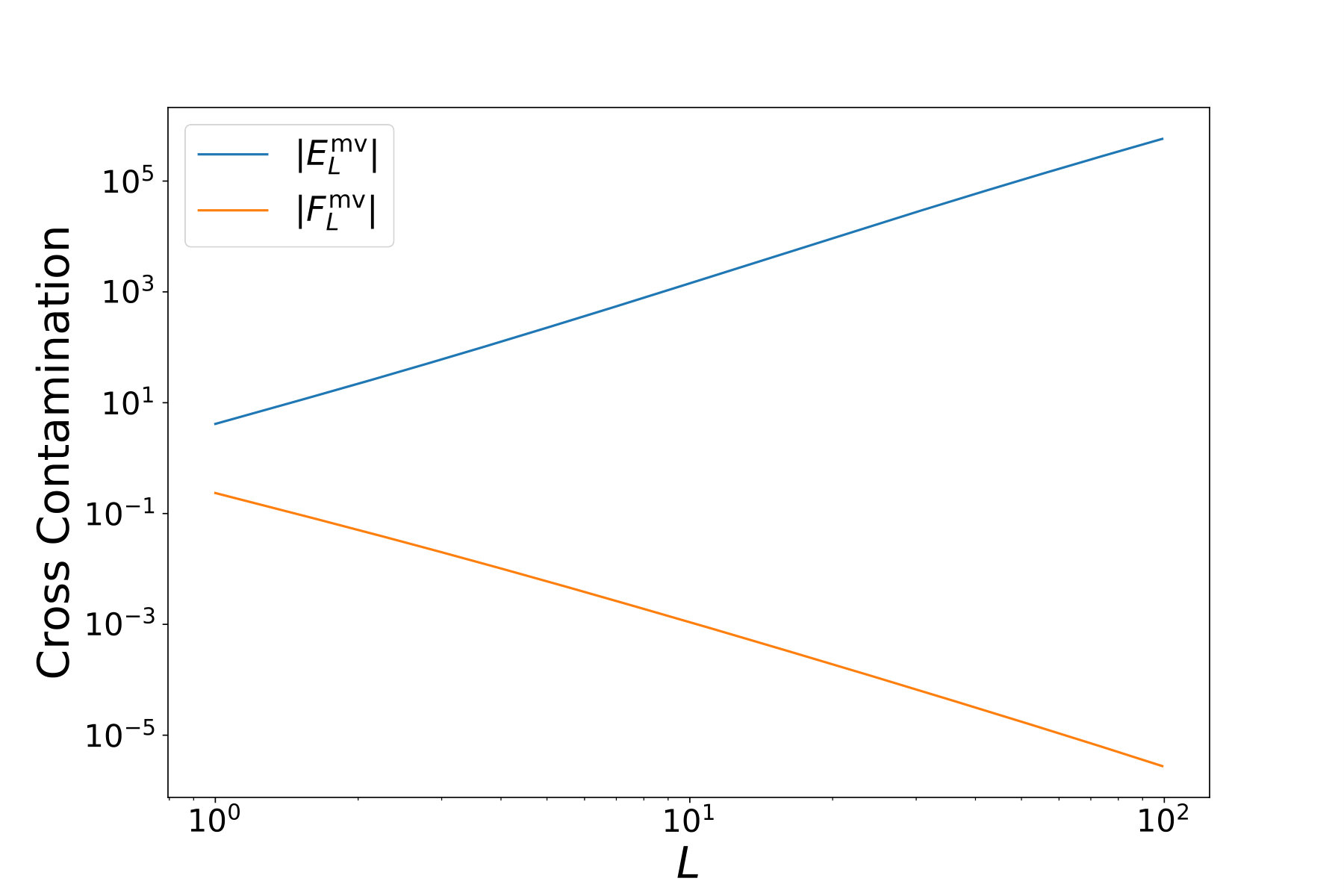 Figure 1
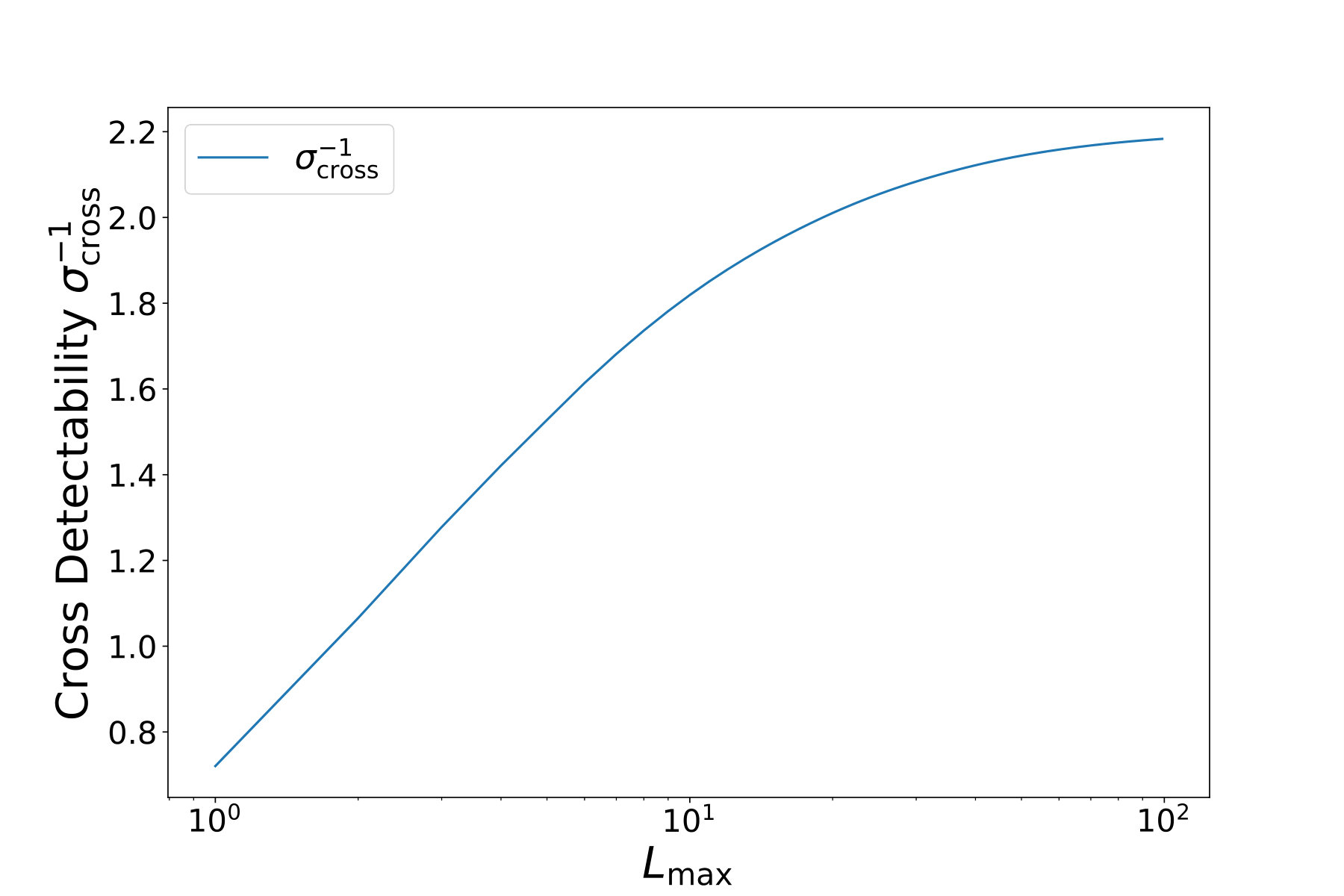 Figure 2
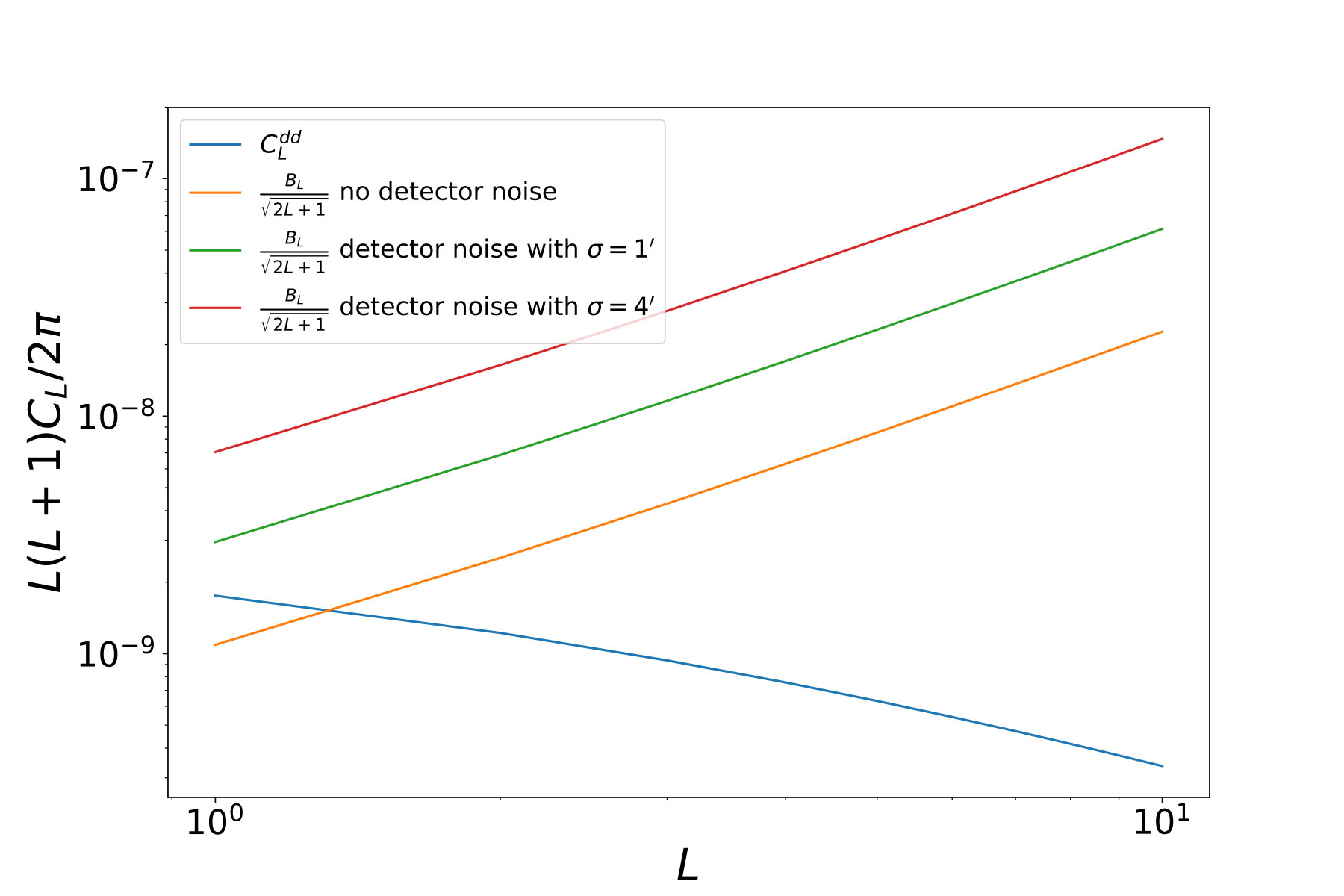 Figure 3
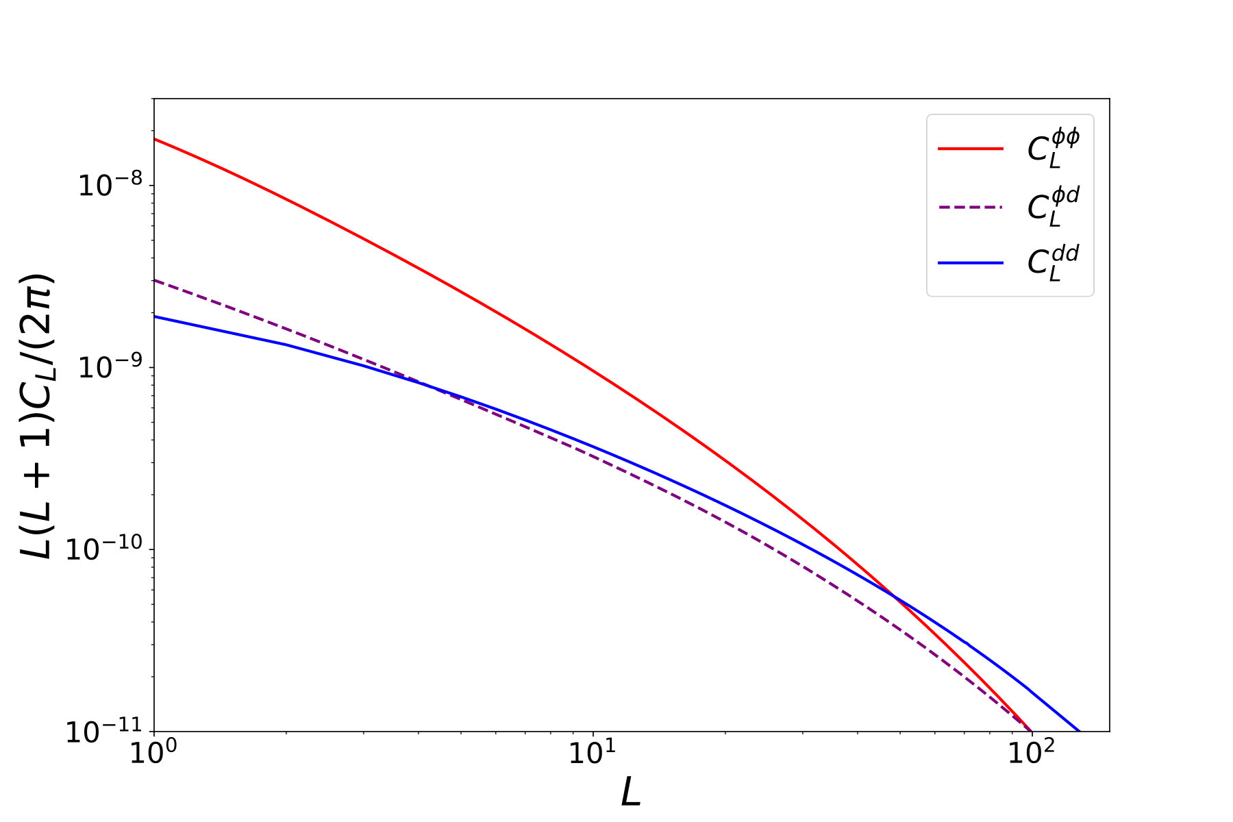 Figure 4
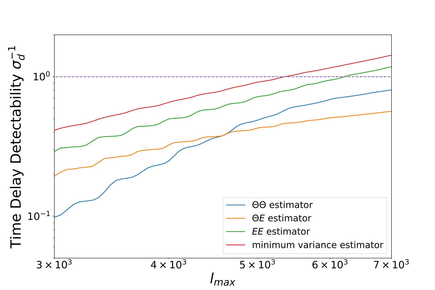 Figure 5
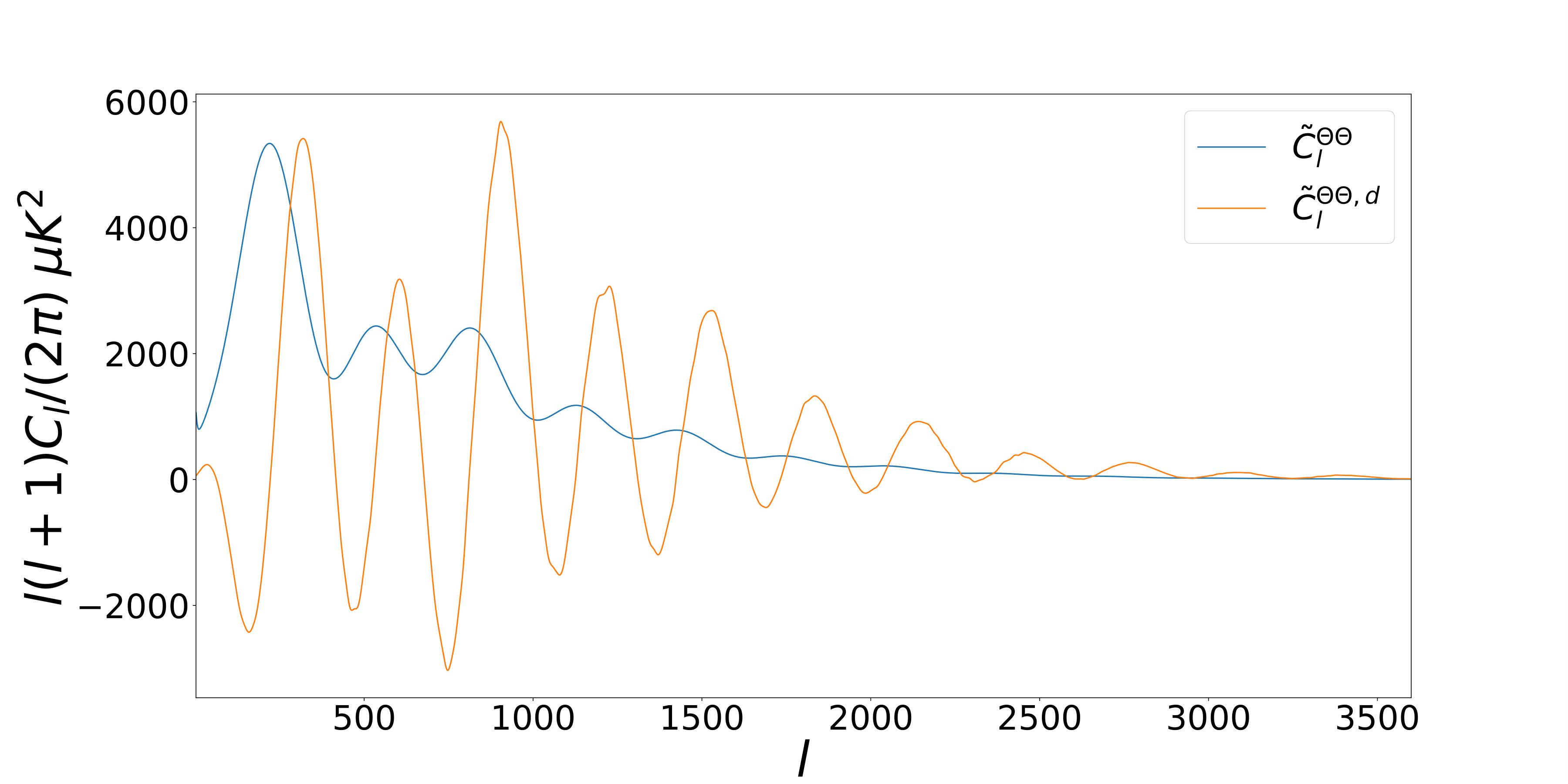 Figure 6
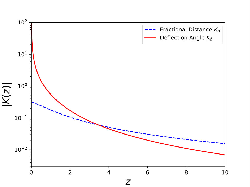 Figure 7
| ] | ||
Peer Reviews
No public reviews on file for this paper yet. If you reviewed it on a platform where reviews are public (OpenReview, ICLR, NeurIPS, ICML), you can paste yours below so the community can read it here.
Videos
No videos yet. Explain this paper in a talk, walkthrough, or lecture? Add one.
Distortions in the Surface of Last Scattering
Peikai Li
Scott Dodelson
Department of Physics, Carnegie Mellon University, Pittsburgh, Pennsylvania 15312, USA
Wayne Hu
Kavli Institute for Cosmological Physics, Department of Astronomy & Astrophysics, Enrico Fermi Institute, The University of Chicago, Chicago, IL 60637, USA
Abstract
The surface of last scattering of the photons in the cosmic microwave background is not a spherical shell. Apart from its finite width, each photon experiences a different gravitational potential along its journey to us, leading to different travel times in different directions. Since all photons were released at the same cosmic time, the photons with longer travel times started farther away from us than those with shorter times. Thus, the surface of last scattering is corrugated, a deformed spherical shell. We present an estimator quadratic in the temperature and polarization fields that could provide a map of the time delays as a function of position on the sky. The signal to noise of this map could exceed unity for the dipole, thereby providing a rare insight into the universe on the largest observable scales.
I Distance to the Last Scattering Surface
The theory of general relativity dictates that particles traveling through gravitational potential wells experience time delays Shapiro (1964). If two photons are emitted at the same time, then they will travel different distances depending upon the potential through which they travel. In the cosmological context of an expanding, spatially flat background, the fractional difference in comoving distance to a source at redshift is
[TABLE]
where is the age of the universe when the photon is a comoving distance from us, and we use the space-time metric convention
[TABLE]
with the scale factor. Note the sign in Eq. (1): if photons pass through an over-dense region where , then they experience a time delay and therefore they arrive from a closer distance than the unperturbed last scattering surface111There is also a geometric time delay that is typically of the same size for a single lens but is much smaller here on the large scales of interest..
Photons that comprise the cosmic microwave background (CMB) experience these same time delays or advances Hu and Cooray (2001) where is the redshift corresponding to the last scattering surface. Since photons do not decouple instantaneously from the electron-proton plasma, the surface of last scattering is often said to have a finite width, and a more accurate expression for the fractional difference in distance traveled is
[TABLE]
where is the Hubble expansion rate; and . Here is the optical depth, ignoring reionization, which becomes very large at times smaller than the epoch of last scattering, or equivalently when .
This directional-dependent change in the distance to last scattering implies that the last scattering surface is not a simple spherical shell. There are two other well-studied phenomena that undercut the notion that the photons in the CMB freely streamed to us from a infinitely thin last scattering sphere. First, since the mean free path at recombination was finite, the last scattering surface has a finite width, and this is accounted for in all computations of CMB anisotropies. Second, the photons in the CMB experience angular deflections as they traverse the inhomogeneous universe Hu (2001); Lewis and Challinor (2006) and this effect has been exploited by recent experiments Smith et al. (2007); Ade et al. (2014); Story et al. (2015); Sherwin et al. (2017); Aghanim et al. (2018) that make maps of the projected gravitational potential.
Although deflections and delays are two different phenomena, they share some similarities, especially in the case of the CMB. Both are determined by the integrated potential along the line of sight, although with slightly different kernels, as depicted in Figure 1: the integrated potential that determines deflections has the same form as the right-hand side of Eq. (3) with
[TABLE]
The corresponding auto and cross power spectra are shown in Figure 2. It is clear that they are highly anticorrelated, so as a first approximation, we might view the maps of the lensing potential created for example in Aghanim et al. (2018) as maps of distance to the last scattering surface. Another similarity, one that has not yet been exploited, is that the quadratic estimator formalism Hu (2001) can be applied to the delays as well, and this is what we will do in this paper. We start though with the rather daunting facts that the RMS fractional distance differences are a factor of ten smaller than the RMS angular deviations and their impact on CMB power spectra is even smaller Hu and Cooray (2001). Further, while the latter peaks at degree scales, the former peak on the largest scales where cosmic variance is higher.
II Effect of distance changes on the CMB
The observed temperature in a given direction is the undistorted temperature plus the deflection due to gravitational lensing plus a term proportional to the small fractional difference . Linearizing these distortions, we obtain
[TABLE]
where is the distance to the radiation sources, here mainly the distance to recombination. We shall see below that we can express this radial derivative in terms of operations on the radiation transfer function. In harmonic space we can write
[TABLE]
with the two first order terms due to deflection and the change in distance equal to
[TABLE]
Notice that both effects couple the undistorted temperature field to the observed temperature field at a different multipole. Here, we have written the integral over the product of three spherical harmonics as and to enable generalization to the case of polarization, which involves spin harmonics. The general expression is
[TABLE]
with
[TABLE]
Note the extra two powers of the multipoles in the function that governs deflection; these follow from the fact that both the temperature and the potential are differentiated with respect to transverse position on the sky. By contrast, the radial derivative that governs the impact of the time delay, or change in distance to the last scattering surface, appears in Eq. (7) as the logarithmic derivative of the undistorted coefficients .
As in the case of the effect of deflections on the CMB, the varying distances to the last scattering surface leads to correlations between -modes that differ from one another. First let us define the power spectrum of the undistorted fields
[TABLE]
where is the radiation transfer function and is the power spectrum of the initial comoving curvature field . Note that the transfer function is a radial integral over the sources at a distance , projected onto multipole moment . We proceed as in Ref. Hu (2001) by focusing on the expectation of off-diagonal () terms quadratic in the observed moments:
[TABLE]
where
[TABLE]
The change in distance to the last scattering produces the spectrum
[TABLE]
This expression is identical to Eq. (10) other than the replacement of one of the transfer functions with
[TABLE]
where the derivative is taken inside of the integrals over the radiation sources by modifying the public CAMB code. The two spectra are shown in Fig. 3.
To clarify the meaning of these terms, consider the large scale limit where the temperature source is the Sachs-Wolfe effect on the recombination surface at , . Then
[TABLE]
More generally the modification to CAMB involves replacing the appropriate Bessel function kernel of the source projection with its log derivative Hu and Cooray (2001).
Note the difference between the two off diagonal correlations in Eq. (11). Each involves a derivative. The one that governs deflections, , involves a derivative with respect to the transverse directions so as defined in Eq. (9) has more powers of than does . The function that governs changes in distances involved a radial derivative, and this shows up in the spectrum .
The correlation between different -modes enables us, following Ref. Okamoto and Hu (2003), to extract information about the fields causing these correlations by forming quadratic estimators out of the observed temperature fields for both the gravitational potential responsible for deflections and the fractional distance field:
[TABLE]
where
[TABLE]
and
[TABLE]
With these definitions, when and when , where the average is over the undistorted CMB fields given fixed distortion fields. To provide an optimistic bound on detectability of the delay distortion, we ignore the cross contamination of the estimators for the time being. We return to this issue in Sec. IV.
The noise on these estimators is now given by the prefactors and , so
[TABLE]
with the first term on the right the signal and the second the noise. Fig. 4 shows the signal and noise at each for several experimental configurations. Here, and throughout, the largest we consider is 7000, as this seems to be within range being considered for a CMB-Stage 4 experiment (see Table 4.1 of Ref. Abazajian et al. (2016)).
An estimate of the detectability of this signal can be obtained by computing the projected error, , on the amplitude of the power spectrum , where the fiducial model has . Approximating the noise as Gaussian gives
[TABLE]
where is the fraction of sky covered by the measurements. Fig. 4 shows that most of the signal comes from the lowest -modes, particularly . However, even for a full-sky experiment and the most optimistic noise projections, the auto power spectrum will not be measurable using temperature only.
III Polarization
The estimator above used only the temperature anisotropy field, but the polarization field contains even more information about the lensing potential that governs deflection and distance changes. This was worked out in detail by Ref. Okamoto and Hu (2003) for deflection, and we follow their notation here. There are now three fields of interest: temperature , and the two fields associated with polarization, and . With letters each ranging over these three fields, we have
[TABLE]
The functions and are the generalizations of Eq. (12) to include polarization (Eq. (12) now corresponds to ). The full set of was determined by Ref. Okamoto and Hu (2003) and is reproduced in Table 1, which now includes the full set of that govern the impact of changing radial distances. Note that
[TABLE]
denotes the power spectra of the undistorted fields with as the radiation transfer function for the field and
[TABLE]
with
[TABLE]
again computed by modifying CAMB. See Ref. Hu and White (1997) for a more detailed discussion. Note that the angular deflection coefficients do not carry superscript d because the derivatives are transverse and therefore captured by powers of .
An estimator can now be constructed for each of the pairs of fields, so letting denote pairs of fields , we have
[TABLE]
where the minimum variance weights are generalizations of Eq. (18)
[TABLE]
Note that in the special cases
[TABLE]
and when (e.g., for or ),
[TABLE]
The covariance of these quadratic estimators
[TABLE]
with Gaussian noise given by
[TABLE]
with , . For , Eq. (30) reduces to . Armed with these expressions, we can form a minimum variance estimator
[TABLE]
with weights and variance given by
[TABLE]
where are the elements of the inverse of the delay noise matrix given by Eq. (30), with matrix indices given by quadratic combinations. Here and below we denote the noise of the minimum variance combination with no indices for simplicity. Analogous expressions with the superscript ϕ apply for the lens potential estimators.
We saw in Fig. 4 that small scale temperature maps only are not sufficient to detect this signal convincingly. To assess the added information contained in the polarization field, we show the detectability in the form of for the lowest -modes (, which contributes essentially all of the signal) as a function for a noiseless experiment in Fig. 5.
Here we keep fixed at for the CMB fields (we tested that our final results are insensitive to this choice) and let vary. We can see that at , the minimum variance estimator detectability reaches 1, and at 7000 is 1.42 but of course this is for the most optimistic of configurations. Note that unlike the minimum variance lensing estimator, the deflection estimator gets little contribution from . This is because the conversion of modes to modes is inefficient in the squeezed limit where , as reflected in the difference between even and odd configurations of the Wigner 3 symbols, and that the modes from lensing provide an intrinsic floor to detectability even in the absence of undistorted modes from gravitational waves.
IV Cross Power Spectrum
The auto-spectrum of the distortion field, , will apparently be very challenging to extract. Another possibility is to cross-correlate the quadratic estimator for the distortion field with other fields that are well-measured. Cross-correlations can be more easily detected if the two-fields are highly correlated and one of the fields can be detected with high signal to noise. Note from Figure 2 that is negative and comparable to the auto spectra and so the two fields and are highly anticorrelated.
As a first attempt, we consider the cross correlation of the -field with the -field responsible for deflections. Without further optimization, the cross-spectrum for the and quadratic estimators is
[TABLE]
where the superscript stands for cross. The noise in the estimators is also correlated because both estimators come from the quadratic combinations of same observables
[TABLE]
We can also construct the analogous noise cross spectrum for the separate minimum variance weighted estimators for and using the weights of Eq. (III)
[TABLE]
Assuming the noise is Gaussian, we can estimate the fractional error on the measurement of the amplitude of the cross spectra from these minimum variance estimators as
[TABLE]
We show this quantity in Fig. 6 where we have set . We see that in this ideal case, could reach about . There are many other lens, and more generally large-scale structure tracers, that delay reconstruction can be correlated with. However the noise here is dominated by , which is common to all such correlations, not or .
Up until this point, we have assumed that the estimators of and are not contaminated by the other so as to provide the most optimistic bound on detectability of the delay distortion. Since the cross power spectrum is potentially measurable at low we conclude by estimating this contamination.
We can define the cross contamination by generalizing the computation in Eq. (18) to retain the distortion induced by on the estimator of and vice versa from Eq. (11) for the average over CMB modes
[TABLE]
where and measure the expected fractional contamination to each estimator in units of their uncontaminated signal rms
[TABLE]
We can then compute minimum variance estimator contaminations using Eq. (31) as
[TABLE]
In Fig. 7 we show the relative contamination fields and for the minimum variance estimators of and respectively. The relative contamination for is large and increases with , reflecting the similar structures in the mode coupling of Eq. (8) but with extra factors of for . Conversely, the relative contamination for decreases with : , . In principle lensing estimators should be corrected for this effect at the lowest . While in the regime relevant to current measurements, the delay contribution to the lens reconstruction is entirely negligible.
If these cross contamination contributions are not removed at the reconstruction level, then the auto and cross spectrum measurements become biased since
[TABLE]
The large contributions from dominate the contamination of the delay auto and cross spectra. For the contamination to measurements, even at the , the renormalization factor in the brackets is about 1.3 and converges to unity rapidly with . To the extent that noise and cross contamination can be neglected in the lensing measurements, the bias can in principle be removed at the reconstruction level without increasing sample variance for the power spectra. In practice this would involve iterating the estimators. However given that the mode coupling forms of Eq. (8) are similar but not identical, especially in the different structures for and , reweighting the triangles to reduce the contamination would be more optimal. Given the relatively low for even perfect removal, we leave these studies to a future work.
V Conclusions
The last scattering surface of the CMB is not purely spherical due to the different travel times experienced by photons as they traverse the inhomogeneous gravitational potential. In principle, these distortions in the distance to different directions is detectable, but we conclude here that the standard auto-correlation techniques will not be sufficient to enable detection in the near future. There is the possibility of cross-correlating a map of the distance distortions constructed with the quadratic estimators introduced here with another map of a closely related integrated potential and extracting the signal in that way. Indeed, this was the way that the transverse distortions in the CMB were first detected Smith et al. (2007). Here, we have considered the cross-correlation signal between the distance distortion and the standard transverse deviation maps and concluded that even an all-sky experiment with superior angular resolution would be detect the combination of auto and cross-spectra at less than 3-sigma. We leave exploration of other cross-correlations and the removal of cross contamination between lensing and delay estimators to future work.
To conclude, we emphasize that a measurement of the matter density on the largest observable scales, which is what a detection of the distance-distortion spectrum (either in auto- or cross-) would provide, carries the potential for enormous insight into the standard cosmological model. The apparent acceleration of the universe is of course a very large scale effect that remains a mystery. Inflation too is deeply embedded in the standard cosmological model and clues to it – or its replacement – might be found by studying the universe on the largest of scales. Over the past decades, a number of large scale anomalies have emerged (see, e.g., the first section of Hansen et al. (2018) for a review of the anomalies) and many ideas for models that might be responsible have emerged. A measurement of CMB deflections and time delays on the largest observable scales could help us either identify one such model or cast further doubt on the standard cosmological model.
Beyond the statistical limitations described in this paper, there are two caveats to the excitement of hunting for large scale physics by studying the distance-distortion. The first is the trivial comment that the deflection spectrum itself carries larger signal to noise even on the largest scales (although not by much, and of course two different measurements would be extremely worthwhile). More important is a physics question regarding the mode, the mode that carries the most signal to noise in the distance-distortion spectrum. In different contexts, there have been arguments that the dipole is suppressed by other effects Zibin and Scott (2008); Itoh et al. (2010). A simple understanding of a large scale gradient in the gravitational potential (i.e., a dipole) would be that all matter experiences the same force and therefore velocity. A simple thought experiment of this “bulk motion” universe suggests that there would still be time delays of the sort described in this paper and the deflections that have been studied previously. However, this may be neglecting other effects that lead to cancellations. This issue too we leave for further study.
Acknowledgements.
We thank Douglas Scott for useful discussions. SD and PL were supported by U.S. Dept. of Energy contract DE-SC0019248. WH was supported by NASA ATP NNX15AK22G, U.S. Dept. of Energy contract DE-FG02-13ER41958 and the Simons Foundation.
The reference list from the paper itself. Each links out to its DOI / PubMed record.
- 1Shapiro (1964) I. I. Shapiro, Physical Review Letters 13 , 789 (1964) . · doi ↗
- 2Hu and Cooray (2001) W. Hu and A. Cooray, Phys. Rev. D 63 , 023504 (2001) , ar Xiv:astro-ph/0008001 [astro-ph] . · doi ↗
- 3Hu (2001) W. Hu, Astrophys. J. 557 , L 79 (2001) , ar Xiv:astro-ph/0105424 [astro-ph] . · doi ↗
- 4Lewis and Challinor (2006) A. Lewis and A. Challinor, Phys. Rept. 429 , 1 (2006) , ar Xiv:astro-ph/0601594 [astro-ph] . · doi ↗
- 5Smith et al. (2007) K. M. Smith, O. Zahn, and O. Dore, Phys. Rev. D 76 , 043510 (2007) , ar Xiv:0705.3980 [astro-ph] . · doi ↗
- 6Ade et al. (2014) P. A. R. Ade et al. (Planck), Astron. Astrophys. 571 , A 17 (2014) , ar Xiv:1303.5077 [astro-ph.CO] . · doi ↗
- 7Story et al. (2015) K. T. Story et al. (SPT), Astrophys. J. 810 , 50 (2015) , ar Xiv:1412.4760 [astro-ph.CO] . · doi ↗
- 8Sherwin et al. (2017) B. D. Sherwin et al. , Phys. Rev. D 95 , 123529 (2017) , ar Xiv:1611.09753 [astro-ph.CO] . · doi ↗