Chemical evolution of galaxies: emerging dust and the different gas phases in a new multiphase code
I. Mill\'an-Irigoyen, M. Moll\'a, and Y. Ascasibar

TL;DR
This paper introduces a new multiphase galaxy evolution model that self-consistently incorporates dust physics, tracking the formation, growth, and destruction of dust alongside gas phase transitions, calibrated against Milky Way data.
Contribution
It presents a novel implementation of dust physics into a multiphase galaxy evolution code with physically motivated conversion rates among gas phases.
Findings
Model aligns with observations at intermediate/high metallicities.
Predicts higher dust content than observed at low metallicities.
Provides a framework for future detailed chemical evolution studies.
Abstract
Dust plays an important role in the evolution of a galaxy, since it is one of the main ingredients for efficient star formation. Dust grains are also a sink/source of metals when they are created/destroyed, and, therefore, a self-consistent treatment is key in order to correctly model chemical evolution. In this work, we discuss the implementation of dust physics into our current multiphase model, which also follows the evolution of atomic, ionised and molecular gas. Our goal is to model the conversion rates among the different phases of the interstellar medium, including the creation, growth and destruction of dust, based on physical principles rather than phenomenological recipes inasmuch as possible. We first present the updated set of differential equations and then discuss the results. We calibrate our model against observations of the Milky Way Galaxy and compare its predictions…
Click any figure to enlarge with its caption.
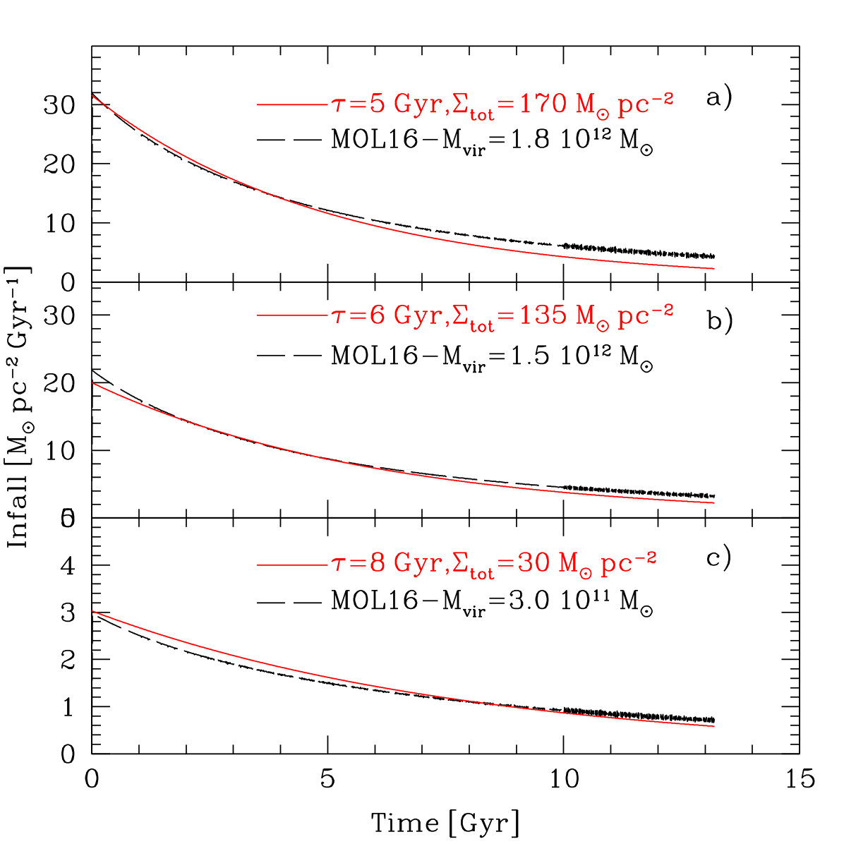 Figure 1
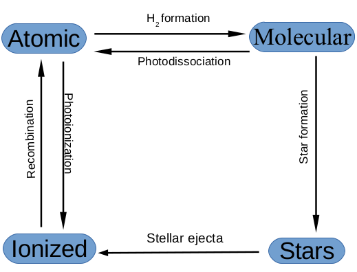 Figure 2
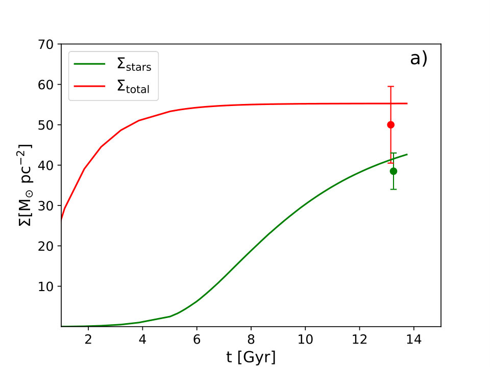 Figure 3
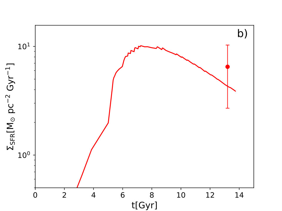 Figure 3
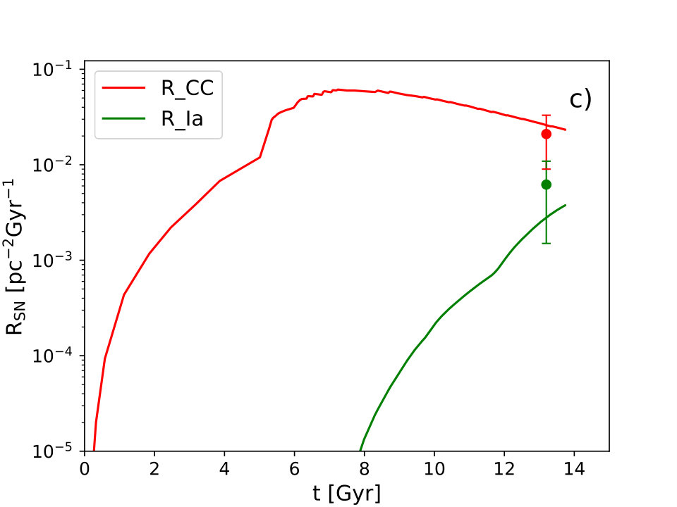 Figure 3
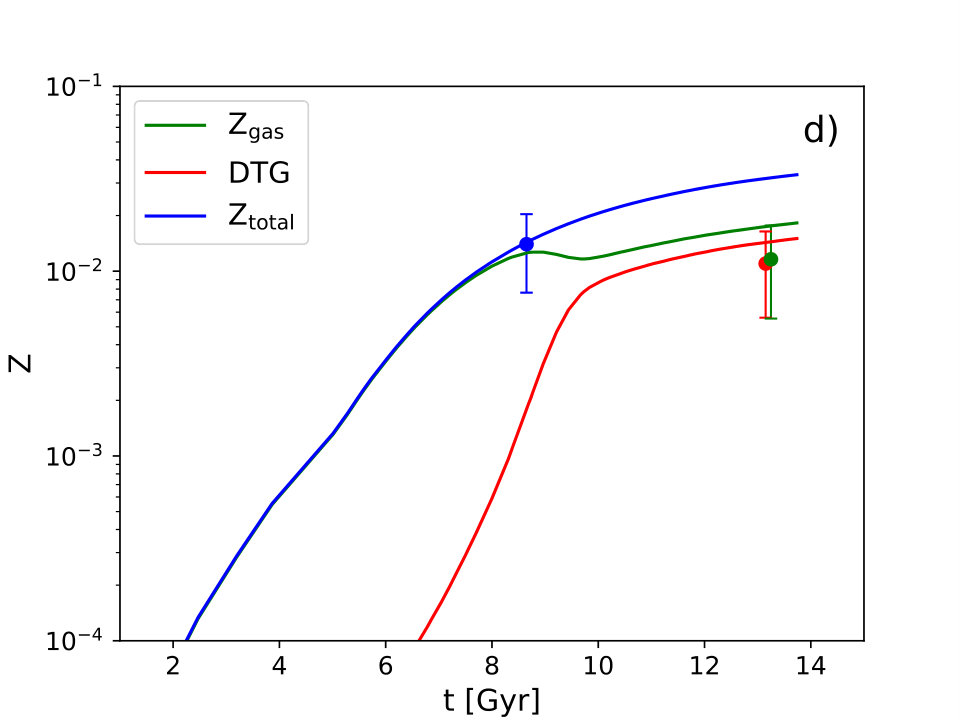 Figure 3
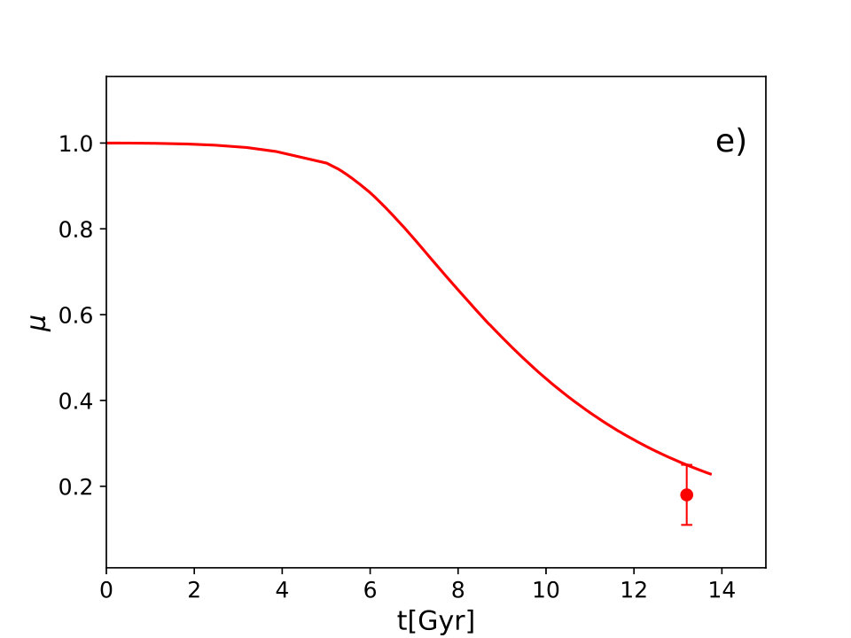 Figure 3
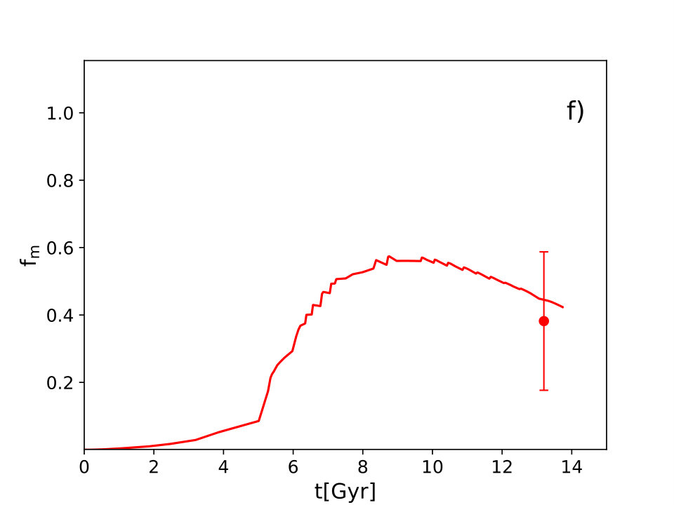 Figure 3
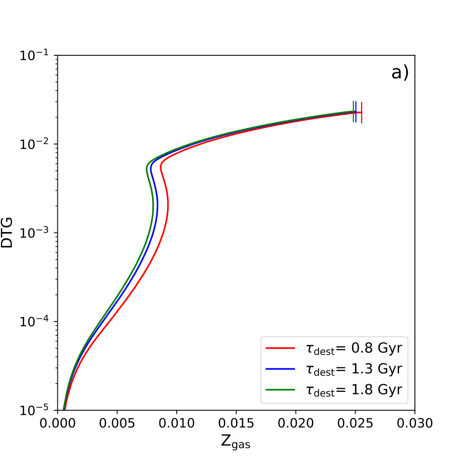 Figure 4
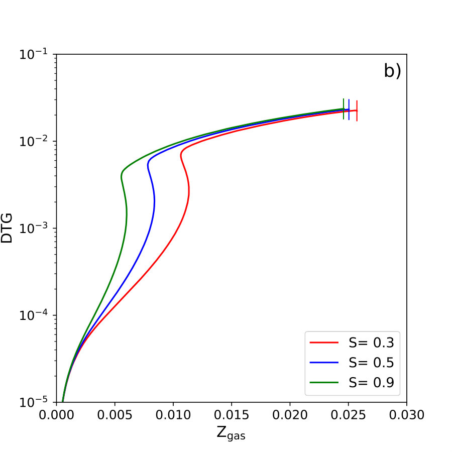 Figure 4
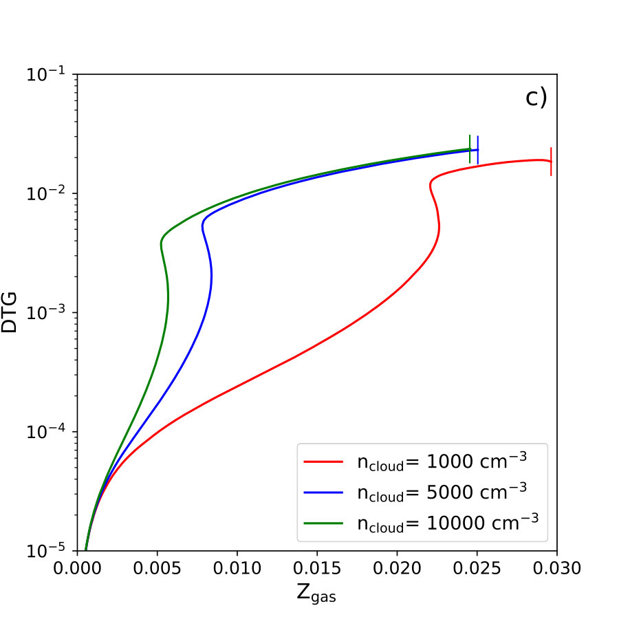 Figure 4
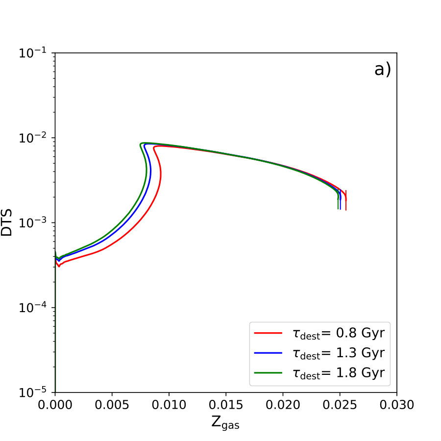 Figure 5
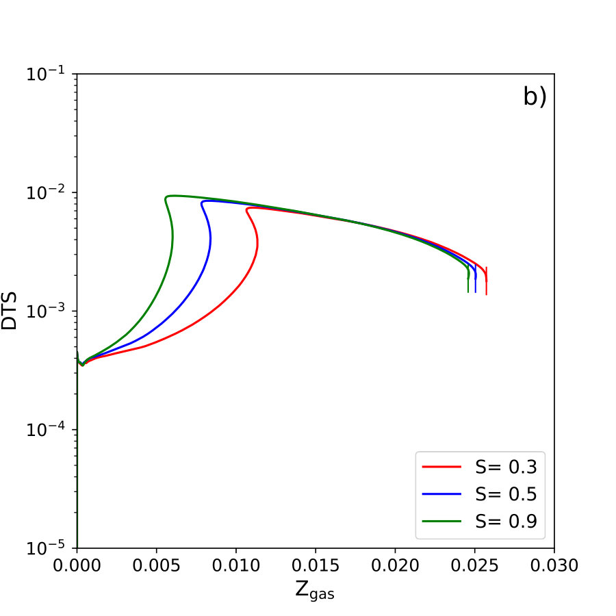 Figure 5
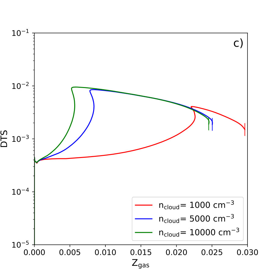 Figure 5
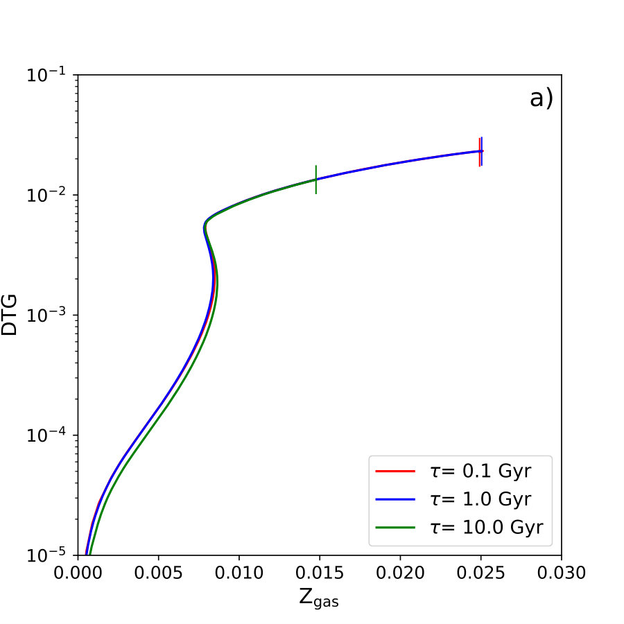 Figure 6
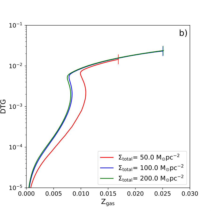 Figure 6
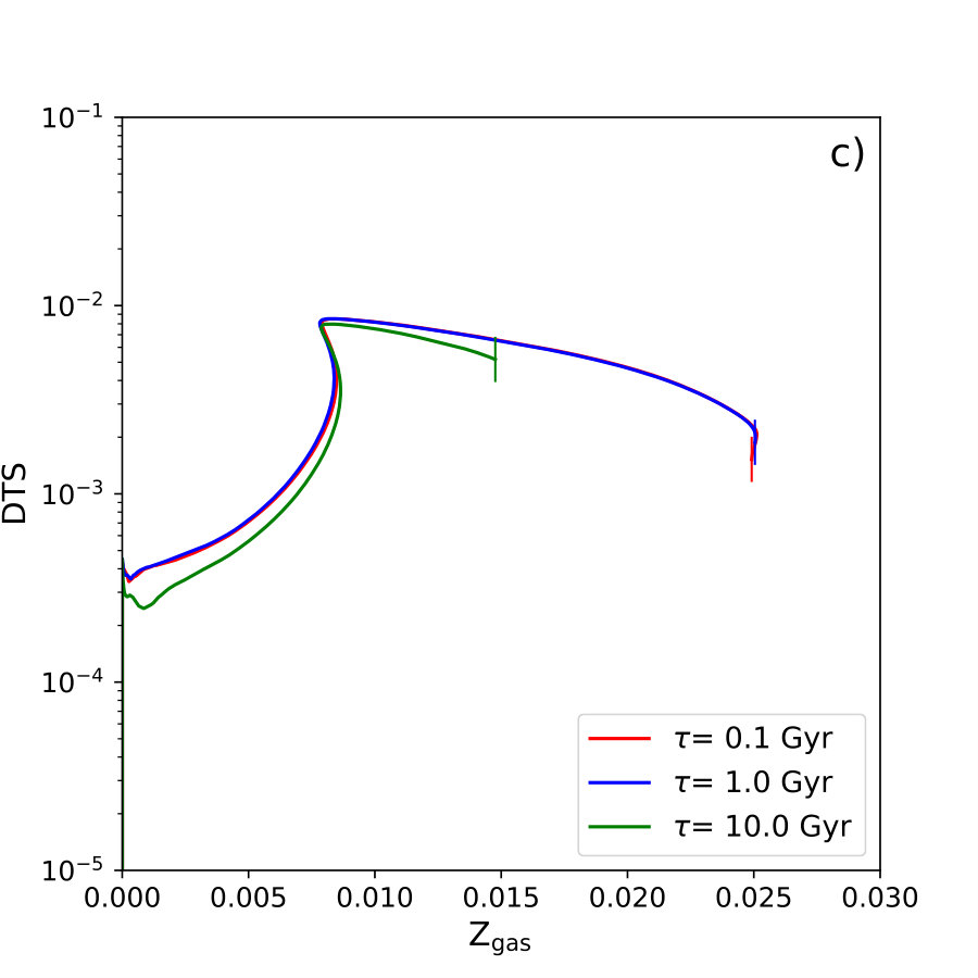 Figure 6
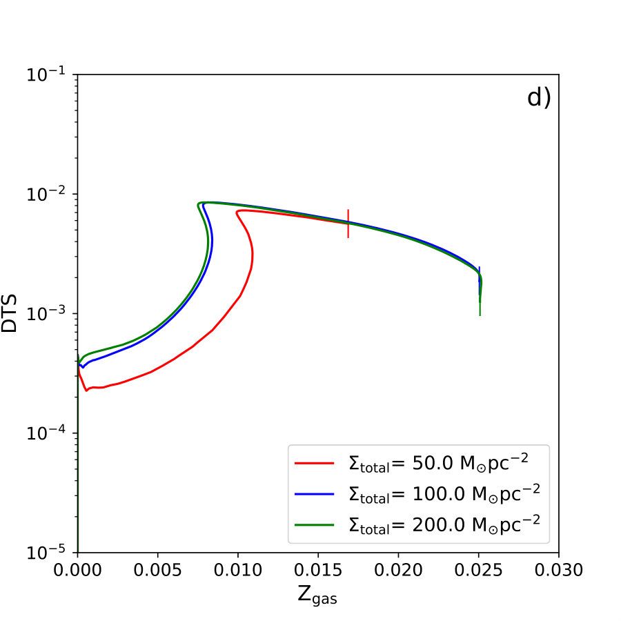 Figure 6
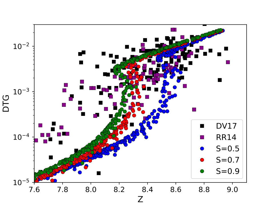 Figure 7
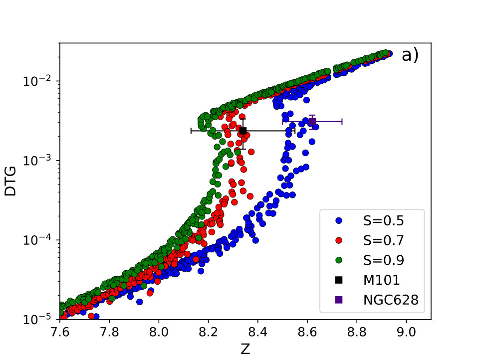 Figure 8
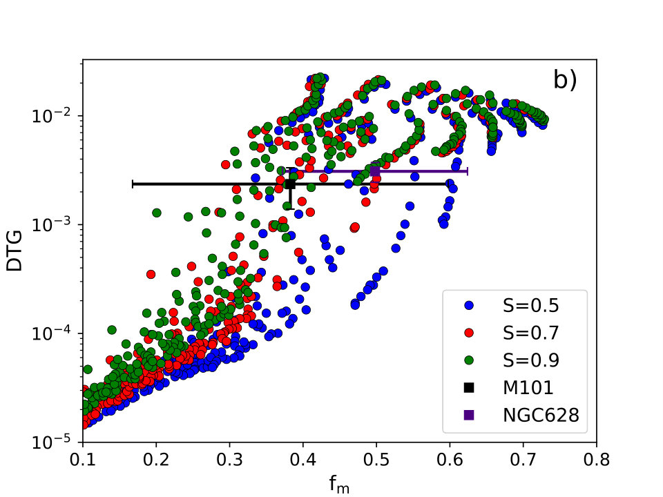 Figure 8
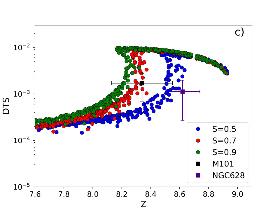 Figure 8
| Symbol | Component |
|---|---|
| Total mass surface density, | |
| Stars and stellar remnants | |
| Interstellar medium, | |
| Gas, | |
| Warm ionised medium | |
| Diffuse atomic gas | |
| Molecular clouds | |
| Hydrogen | |
| Helium | |
| Metals in the gas phase | |
| Dust |
| Dust parameters | range |
|---|---|
| S | |
| Gyr | |
| Infall parameters | range |
| Gyr | |
| [10.0,200.0] |
| Data | Value | Ref. |
|---|---|---|
| 55 10 | M15 & BO17 | |
| 38.5 2.5 | BO17 | |
| 5.3 4.0 | M15 | |
| 0.15 0.08 | M15 | |
| 0.0208 0.0118 | T94 | |
| 0.0062 0.0047 | T94 | |
| 0.4 0.2 | M15 | |
| 0.0106 0.007 | F03 | |
| 0.014 0.008 | ASP09 | |
| 0.011 0.007 | EST19 |
Peer Reviews
No public reviews on file for this paper yet. If you reviewed it on a platform where reviews are public (OpenReview, ICLR, NeurIPS, ICML), you can paste yours below so the community can read it here.
Videos
No videos yet. Explain this paper in a talk, walkthrough, or lecture? Add one.
Chemical evolution of galaxies: emerging dust and the different gas phases in a new multiphase code
I. Millán-Irigoyen1, M. Mollá,1 and Y. Ascasibar2,3
1 Departamento de Investigación Básica, CIEMAT, Av. Complutense 40,E-28040, Madrid, Spain
2 Departamento de Física Teórica, Universidad Autónoma de Madrid, E-28049, Cantoblanco (Madrid), Spain
3 Astro-UAM, Unidad Asociada CSIC, Universidad Autónoma de Madrid, E-28049, Cantoblanco (Madrid), Spain E-mail: [email protected]: [email protected]: [email protected]
(Accepted XXX. Received YYY; in original form ZZZ)
Abstract
Dust plays an important role in the evolution of a galaxy, since it is one of the main ingredients for efficient star formation. Dust grains are also a sink/source of metals when they are created/destroyed, and, therefore, a self-consistent treatment is key in order to correctly model chemical evolution. In this work, we discuss the implementation of dust physics into our current multiphase model, which also follows the evolution of atomic, ionised and molecular gas. Our goal is to model the conversion rates among the different phases of the interstellar medium, including the creation, growth and destruction of dust, based on physical principles rather than phenomenological recipes inasmuch as possible. We first present the updated set of differential equations and then discuss the results. We calibrate our model against observations of the Milky Way Galaxy and compare its predictions with extant data. Our results are broadly consistent with the observed data for intermediate and high metallicities, but the models tend to produce more dust than observed in the low metallicity regime.
keywords:
Galaxies: evolution – ISM: dust, extinction – Galaxies: abundances
††pubyear: 2019††pagerange: Chemical evolution of galaxies: emerging dust and the different gas phases in a new multiphase code–A
1 Introduction
Until the mid- century, cosmic dust was, for most astronomers, a foreground that complicated the observation of distant objects. When the first observations in the infrared became available, the chemical composition and distribution of dust in the interstellar medium (ISM) could be measured, and theories about its role in the evolution of galaxies emerged. Nowadays, it is widely known that interstellar dust is made up of very small solid particles (grains of in size) of carbon, silicates and ices from other chemical species. It is also estimated that the entire mass constituting the ISM represents % of the total baryonic mass of a galaxy, of which % corresponds to gas, with only 1% attributed to dust.
The so-called "dust cycle" consists essentially on the following processes (see Zhukovska, Gail & Trieloff, 2008, hereafter Z08), c.f. (Asano et al., 2013; Gioannini et al., 2016):
Ejection from stars and injection into the ISM. 2. 2.
Evolution: production in the ISM, growth and destruction. 3. 3.
Star formation: molecular cloud formation and shielding.
Most theoretical models of dust formation are based on the condensation of metallic elements from their gaseous phase in a solid state through nucleation processes (Feder et al., 1966; Todini & Ferrara, 2001; Nanni et al., 2014). For the condensation to happen, the partial pressure in the gas has to be greater than the vapour pressure in the condensed phase (Valiante et al., 2009). The size of the grains basically depends upon three parameters related to the thermodynamic conditions: the gas temperature (), the gas pressure () and the condensation temperature of the involved chemical species ().
Nucleation occurs in a range of between and Pa, with K, and these restrictive conditions limit the possible sources of dust grains observed in the ISM. There is a consensus that the major sources of dust in the Universe are stars of low and intermediate mass () having evolved through the asymptotic giant branch i.e., AGB stars (Z08, Ventura et al., 2012a, b; Di Criscienzo et al., 2013; Nanni et al., 2013; Dell’Agli et al., 2015, 2017; Ginolfi et al., 2017), as well as massive stars () when they die as core-collapse type II SNe (CC-SNe; Todini & Ferrara, 2001; Schneider, 2004; Nozawa et al., 2007; Bianchi & Schneider, 2007; Cherchneff & Dwek, 2009, 2010; Marassi et al., 2014, 2015; Sarangi & Cherchneff, 2015; Bocchio et al., 2016; Ginolfi et al., 2017).
It has been argued (see e.g. Morgan & Edmunds, 2003; Valiante et al., 2009; Gioannini et al., 2016) that other sources are necessary in order to reproduce the amounts of dust observed in the Universe, and many candidates have been proposed, such as SNe type Ia (Nozawa et al., 2011), red giant branch (RGB) stars (Origlia et al., 2010), luminous blue variable (LBV) stars (Z08), Wolf-Rayet (WR) stars (Zhekov et al., 2014; Cherchneff, 2015) or even Population III stars passing through their red supergiant (RSG) phase (Marassi et al., 2015).
After nucleation, dust undergoes different evolutionary processes in the ISM. Some of these processes change the dust mass, such as growth by accretion (e.g. Inoue, 2011; Zhukovska, 2014; Zhukovska et al., 2016; Zhukovska, Henning & Dobbs, 2018) or its destruction by thermal or chemical sputtering, while others modify its properties (e.g. the shattering or fragmentation by grain collisions, which can affect the size distribution). Eventually, dust grains are incorporated into the next generations of stars (astration) or destroyed by either thermal pulverisation produced by the reverse shock in SN explosions (e.g. Bianchi & Schneider, 2007; Nozawa et al., 2011) or the radiation field surrounding very luminous objects (e.g. Hoang et al., 2018).
Despite the insignificance in the mass budget of a galaxy, the importance of the dust component can hardly be overstated. Besides its impact on the observed spectral energy distribution (through the absorption, emission and scattering of photons at different wavelengths), the presence of dust grains plays a central role in the chemical evolution of any galactic region, as well as of the galaxy as a whole, since dust regulates the creation of molecules in the ISM and the shielding of molecular clouds from ultraviolet (UV) photons.
Over the years, several theoretical models have appeared that account for the abundance of one or more dust species simultaneously with the chemical elements in the gas phase of the ISM (e.g. Dwek, 1998; Calura, Pipino & Matteucci, 2008; Inoue, 2011; Asano et al., 2013; Zhukovska, 2014; Gioannini et al., 2016; Zhukovska et al., 2016; Zhukovska, Henning & Dobbs, 2018).
Building upon these studies, the main aim of the present work is to discuss the implementation of dust physics into a multiphase chemical evolution model. This represents a significant improvement with respect to previous works; in some of the latter (e.g. Mollá et al., 2015, 2016, 2017), the availability of molecular gas is one of the main ingredients of the star formation process, but the dust phase is not included. In others, the dust is taken into account, but only crudely modelled, with the assumption that the dust mass scales approximately linearly with the metal content, according to some proportionality constant that was fitted as a phenomenological parameter. Here, we will describe and test a physically motivated formalism that provides a much more realistic (and significantly more constrained) parametrization, and opens the possibility of testing the model results against dust-related observational data, increasing the predictive power of the models and helping to break the degeneracies intrinsic to chemical evolution studies.
Our new model is fully described in Section 2, where we explain in detail the equations that determine the transfer of mass between the different phases and the precise meaning of the small number of free parameters that appear only in the dust physical or phenomenological prescriptions. After deriving our system of coupled differential equations, we can obtain the time evolution of the gas (including diffuse, ionised and molecular phases), stars, metals and dust densities in a given galaxy. Including a careful treatment of the dust life cycle based on first principles is particularly important in relation to the phase balance and the star formation processes, since the main channel for the creation of hydrogen molecules is the condensation onto the surface of dust grains.
The first results of the model are presented in Section 3, where we discuss the time evolution of a fiducial configuration that is representative of a Milky Way Galaxy (MWG) or solar neighbourhood-type model. After verifying that we are able to successfully reproduce the local environment, we study the effect of varying the dust-related parameters (destruction timescale, cloud density, and sticking coefficient) and of changing the main inputs of the model (the total mass surface density and the infall timescale), which define a given size of galaxy, in order to disentangle their contribution to the evolution and the final outcome of the model. Finally, we compare the results of a model grid covering a broad range of parameter values with a set of observational data of dust abundances in external galaxies available in the literature. Our man conclusions are summarised in Section 4.
2 Model Description
The main aim of chemical evolution models is to describe the temporal evolution of different chemical species within a galaxy,in order to confront the predicted behaviour with that observed. In our model, we consider that galaxies have a multiphase structure that includes neutral, ionised and molecular gas phases in the ISM, and we follow the abundance of hydrogen, helium, metals and dust. The equations that determine the evolution of each component will be discussed in subsections 2.1, 2.2 and 2.3. In order to compare our theoretical predictions with observations, the mass content of all phases is expressed in terms of surface density.
A summary of the phase-dependent notation adopted herein is provided in Table 1. The total mass of each galaxy is defined as the sum of the stellar and ISM mass. This ISM, in turn, is composed of warm ionised gas, diffuse atomic gas, and molecular clouds. Within the gas, metals appears as a consequence of the evolution and death of stars. Thus, its composition is , where, as usual, is the mass abundance of , is the mass abundance of and is the mass abundance of all the remaining elements. In our scenario, we start with a disk of zero total mass, , and consider infall of gas from outside with primordial abundances (Coc et al., 2012) that replenishes the disk galaxy. At the end of our runs (13.2 Gyr as in Mollá et al., 2015), a disk remains with characteristics consistent with those observed in nearby spirals.
2.1 Gas
Since the ISM in a galaxy is not homogeneous, it is indispensable to model it as a multiphase structure. For that purpose, we have considered: a) an ionised phase with a temperature of K, b) an atomic component whose temperature is K, and c) a molecular phase with a temperature of K. These phases interchange mass with each other during the evolution of the region under study. The processes involved are: the photoionisation of atoms, the recombination of electrons with ions, the conversion of atomic hydrogen into molecular hydrogen and the destruction of the latter due to the photodissociation caused by UV light from the young stellar population. In addition, the studied region/galaxy can accrete mass from the outer regions and/or from the Intergalactic Medium (IGM) via infall. We define each one of these phases, and the processes they suffer from, in the following subsections.
2.1.1 Infall
Since we are not considering a closed-box model for our galaxy, it is necessary to take into account the interaction with its environment. This interaction can make the region either gain mass, via infall, or lose mass due to galactic outflows. As shown in Gavilán et al. (2013), the observed properties of many galaxies can be reproduced by chemical evolution models without an outflow component, and therefore we have only included infall in the present tests in order to minimise the number of free parameters. With this model, we will assess whether the basic relations involving the dust abundance ratios, as observed in the local Universe, may be qualitatively reproduced and understood in terms of the underlying physical processes. More complicated models aimed to provide a detailed match to particular objects and/or other galaxy types will be explored in our future work.
Here we have considered, for the sake of simplicity, that the infall rate from the IGM can be approximately described by an exponential law:
[TABLE]
which depends on two parameters, the infall timescale, , controlling the infall rate, and , the final total surface density of the region under study at . These quantities, and , which fully define the infall rate, are model inputs meaning that they must be changed to represent different galaxies or regions
According to Eq. (1), if , the majority of the gas will have already infallen on a rapid timescale. On the other hand, if , the gas will fall at an approximately constant rate. The above expression captures the main features of more realistic infall rates obtained in other models and cosmological simulations.
We show in Fig. 1, three different combinations of and , as labelled in each panel, compared with the infall rates used in Mollá et al. (2016) for galaxies of different virial masses/sizes. We assume that this gas falling into the galaxy is ionised, since it comes directly from the IGM and/or from a hot galactic halo, where the temperature is well above K. Furthermore, the gas has primordial abundances, i.e., and , (Coc et al., 2012). This assumption of primordial abundances may not be entirely correct for fountain material mixed with coronal material infalling back onto the disk as explored in Gibson, et al. (2002); however, it is probably sufficient as a first order hypothesis.
2.1.2 Recombination
The gas in the ionised phase will capture free electrons and become neutral on a characteristic recombination timescale:
[TABLE]
where denotes the electron number density at time , and cm3 s*-1* corresponds to the thermally-averaged Case-B recombination cross-section (i.e. without considering transitions to the ground state) appropriate for a temperature of the ionised phase of K (Osterbrock & Ferland, 2006).
2.1.3 Molecular hydrogen formation
The conversion of atomic into molecular hydrogen is another relevant physical process given the importance of the molecular phase in the star formation process (see Section 2.2.1). There are several channels for the creation of H2 molecules in the diffuse ISM, such as:
[TABLE]
Due to the low abundance of negative ions in the ISM, these reactions have very slow rates. Other channels, such as the three-body reactions that take place in the Earth’s atmosphere, are strongly suppressed at astrophysical densities, and the most efficient processes for the formation of involve the interaction of H atoms on the surface of dust grains, which are regulated by the timescale:
[TABLE]
where is the volume density of dust grains in the ISM, and is the thermally-averaged cross-section for the formation of molecular hydrogen (see e.g. Tielens & Hollenbach, 1985; Draine & Bertoldi, 1996; Cazaux & Spaans, 2004).
According to Glover & Jaspen (2007), formation in grains becomes dominant as soon as . This value is so low that a detailed treatment of other channels would have a minimal impact on the results, but it would be necessary to include them in the model in order to start the process, since the initial abundance of metals and dust grains is zero, and stars only form from molecular clouds. We circumvent this problem, (as in Mollá et al., 2017), by adding the minimum metallicity to the value of the ISM when estimating the timescale for cloud formation. This way:
[TABLE]
where denotes the gas density, is the solar metallicity (Asplund et al., 2009), and is the rate of molecular hydrogen formation given by Draine & Bertoldi (1996) for K. This is an approximation that could be eliminated in future work by explicitly model the mechanisms responsible for the formation of molecular clouds in the low-metallicity regime.
2.1.4 Photoionisation and Photodissociation
In order to estimate the photoionisation rate of H atoms at each time step , we compute the number of ionising photons produced in the galaxy per unit time by summing the contribution:
[TABLE]
of different Single Stellar Populations (SSPs) of age and metallicity , where is the specific luminosity per unit wavelength per unit mass of the SSP, is the Planck constant, and is the speed of light. The total rate of ionising photons at time is:
[TABLE]
may be obtained by integration over the star formation history and chemical evolution of the galaxy.
Since most of the ionising radiation of a SSP comes from young blue stars that die in the first Myr, it is possible to approximate and obtain a constant photoionisation efficiency per unit Star Formation Rate (SFR):
[TABLE]
Taking the values of tabulated for the POPSTAR code (Mollá, García-Vargas & Bressan, 2009) for SSPs with ages between and , we obtain for a Kroupa (2001) IMF.
In order to obtain the efficiency of photodissociation of into , we perform a similar computation for the radiation emitted by each SSP in the Lyman-Werner band:
[TABLE]
However, Draine & Bertoldi (1996) showed that dust grains may absorb up to of the photons capable of dissociating hydrogen molecules, and a large fraction of the remaining photons actually excite different rotational and vibrational states, reducing their dissociation probability to . Therefore, the net photodissociation efficiency per unit SFR should be of the order:
[TABLE]
From the aforementioned considerations, we see that the conversion of phases can be defined without the need for any free parameters.
2.2 Stars
2.2.1 Star formation
The birthrate, i.e., the amount of stars of each mass that have been created per unit time and per unit area, is usually decomposed (Pagel, 2009) as:
[TABLE]
where is the SFR, defined as the mass in newly-born stars created per unit time, and is the initial mass function (IMF).
Despite its crucial importance in galactic evolution, there is not a precise theoretical model that takes into account all the effects associated with star formation. Thus, the use of empirical laws to define the SFR is the traditional approach employed. Usually, these laws relate the SFR with the local (two- or three-dimensional) density of the gas. One of the most common prescriptions is the Kennicutt-Schmidt law based on Schmidt (1959) and Kennicutt (1998). The Kennicutt-Schmidt law is expressed by the well known formalism: , where (t) is the surface density of gas and is an exponent whose best-fitting value is .
However, there have been studies suggesting that the correlation between SFR and molecular gas surface density is stronger than the one between SFR and total gas surface density, (see e.g. Wong & Blitz, 2002; Krumholz & Thompson, 2007; Robertson & Kravtsov, 2008; Bigiel et al., 2008; Krumholz, McKee & Tumlinson, 2009; Bigiel et al., 2010; Bolatto et al., 2011; Schruba et al., 2011; Krumholz, Dekel & McKee, 2012; Leroy et al., 2013), which is reasonable since it is clear that stars form within cold molecular clouds. Therefore, given that our model considers the multiphase structure of the galactic region/galaxy, we prefer to use a relationship between the SFR and the molecular gas density, such as: where is the mass surface density of the molecular phase and is a characteristic timescale of star formation.
There are uncertainties in the value of and its possible variability, depending on the medium where star formation is happening. On the observational side, Bigiel et al. (2008) studied 7 spiral and 11 late-type/dwarf galaxies and found a mean value of Gyr, detecting differences between the centre and the outskirts. In fact, Bigiel et al. (2010) observed later the outer part of the disks of spiral galaxies and concluded that is even higher than the Hubble time in these outer regions; (Bolatto et al., 2011) estimated a slightly shorter Gyr, with significant variations (ranging form 0.6 to 7.5 Gyr) throughout the Small Magellanic Cloud. Finally, Leroy et al. (2013) have obtained a value Gyr from observations of 30 nearby disk galaxies. Consequently, there have been some attempts to make empirical laws considering different depletion times depending on the environment, such as Krumholz, McKee & Tumlinson (2009), whose empirical law depends on the surface density of the ISM where the star formation occurs. We are going to use here the expression given by these last authors:
[TABLE]
The IMF is the observational distribution of the number of stars according to their initial masses in every star formation event. There are also some uncertainties in the exact shape of the IMF, particularly in the low and high mass regime due to the difficulties of observing stars with extremely low masses and to the rapid death of massive stars. In this work, we have assumed an IMF from Kroupa (2001), with the following expression:
[TABLE]
where and are the normalisation constants, for a minimum stellar mass of and a maximum stellar mass of , which give . Our upper limit was chosen in order to minimise the extrapolation of Woosley & Weaver (1995) ejecta, which are provided up to 40 M⊙, and it agrees with the upper limit found or used by other authors (e.g. Kobayashi & Nakasato, 2011; Mishurov & Tkachenko, 2018, 2019). 111Furthermore, for the adopted IMF, the contribution of stars above this limit to the total ejecta budget is negligible. See section 2.2.3.
2.2.2 Mean stellar lifetimes
Instead of using the instantaneous recycling approximation, we will take into account the lifetimes of the stars with the empirical formulae provided by Raitieri, Villata & Navarro (1996), calculated from different stellar tracks (Alongi et al., 1993; Bressan et al., 1993; Bertelli et al., 1994) over a stellar mass range of [ - ] and a metallicity range of [ - ]:
[TABLE]
where denotes the lifetime of a star of mass and metallicity , and the coefficients , and are given by the following expressions:
[TABLE]
2.2.3 Stellar ejecta
The chemical composition of the gas ejected by a star at its death is different from the one of the molecular cloud from which it formed, as the material has been enriched with the elements that have been created in the interior of the star via nucleosynthesis. For our chemical evolution model, we are interested in the total (gas and dust) ejection rate of each element as a function of time , which we divide in three components:
[TABLE]
where , and denote the contributions of low- and intermediate-mass stars, high mass stars and type Ia SNe, respectively.
Low and intermediate mass stars end their lives as planetary nebulae after passing the Asymptotic Giant Branch (AGB) phase, during which the star loses an important fraction of its mass. These objects eject to the ISM mainly , , and . The ejection rate for each element is computed as:
[TABLE]
where is the minimum mass of a star of metallicity Z to have died prior to the moment . These stars are born at a time , according to equation (15) above. is the SFR of the galaxy/region at that time, and is the assumed IMF. For the mass returned by a low and intermediate mass star with mass and metallicity at the end of its life in form of element , we use the tables provided by Mollá et al. (2015).
The final fate of high mass stars () is that of an explosion as core-collapse supernova. These supernovae are responsible for ejecting the so-called -elements (i.e., 12C, 16O, 20Ne, 24Mg, 28Si, 32S and 40Ca) created in the interior of these massive stars during their evolution, as well as unstable isotopes of Ti, Cr, Fe and Ni, created during the explosion itself, whose decay provides a significant fraction of the energy that is radiated away during the explosion.
At any given time, the rate of core-collapse supernova explosions is given by:
[TABLE]
and the ejection rate of element is simply
[TABLE]
where is the total mass that a massive star of mass and metallicity returns as element at the end of its life taken from Woosley & Weaver (1995)222These tables have been extensively used in the literature, and there is little difference in the oxygen yields up to with respect to more recent prescriptions (Mollá et al., 2015)..
Finally, the third mechanism that ejects newly synthesised metals to the ISM is the thermonuclear explosion of type-Ia supernovae. Although some other chemical species are produced, their main contribution is the synthesis of iron-peak elements (Ti, V, Cr, Mn, Fe, Co and Ni), being the principal mechanism for iron enrichment in galaxies.
In order to compute the ejecta of type-Ia supernovae, we need their rate of occurrence:
[TABLE]
where dm is the number of stars per unit mass in a stellar generation, is the fraction of (binary) systems that end up as a thermonuclear SN, and DTD is the Delay Time Distribution that describes how many type Ia SNe progenitors die after a at time . The lower limit of the integral is the minimum delay time , whereas the upper limit is the minimum between the maximum delay time and the current age of the galaxy. We use a constant for the Kroupa IMF (Maoz & Hallakoun, 2017) and the empirical DTD from Maoz & Gaur (2017). The precise shape of the DTD is a very active research topic, with some slight differences of the empirical functions with respect to theoretical predictions (e.g. Greggio, 2005). These latter properly account for stellar lifetimes, binary fractions, and evolution, while the first ones are easy to use, but not totally correct at the shortest phases of the evolution ( Myr). However, since we are not computed relative abundances of different chemical species, as , but only the whole metallicity Z, it is unlikely that these differences would produce a significant effect in the present context.
Once the supernova rate is determined, the ejection rate of type Ia supernovae is:
[TABLE]
where are the ejecta of element in each SNIa, for which we adopt the yields of the classical model W7 from Iwamoto et al. (1999).
With these three definitions, the amount of mass per unit time that stars inject into the ISM in the form of hydrogen and helium will be denoted by and , respectively. As will be discussed below, the total ejection rate of metals:
[TABLE]
will distinguish between the gaseous and dust phase, .
2.3 Dust
Given the relevance of the dust in some key processes of galactic evolution, it is important to model correctly its life cycle. As noted previously, dust grains are mainly created in the AGB phase of low and intermediate mass stars () and at the final stage of the shock waves produced by core-collapse and thermonuclear SNe. Several authors (e.g. Z08, Zhukovska et al., 2016; McKinnon, Torrey & Vogelsberger, 2016; Gioannini et al., 2016; Aoyama et al., 2017; Zhukovska, Henning & Dobbs, 2018) have argued that in order to reproduce the observed values of the dust to gas ratio, it is necessary that dust grains accrete mass from the ISM333In addition to the dust growth by accretion, dust grains suffer a variety of effects in the ISM that change their size, such as shattering, coagulation, etc. They are not considered here, since we assume an unchanging Mathis, Rumpl & Nordsieck (1977)’s grain size distribution.. Finally, we also consider that the grains may be destroyed by SN shock waves, thermal sputtering, radiative torques and astration444Mass loss of certain chemical element or dust species due to its incorporation to a star during a SF process.
2.3.1 Dust creation
The creation of dust grains inside the atmosphere of low- or intermediate-mass stars is not significant until they reach the AGB phase (Gail, 2009). Afterwards, they are considered to be the main stellar contributors to dust enrichment in the ISM. At any given moment , the total mass of dust ejected per unit time is given by:
[TABLE]
where is the dust ejecta for a star of mass and metallicity . Yields are taken from Ventura et al. (2012a, b); Di Criscienzo et al. (2013); Dell’Agli et al. (2017).
Secondly, we have to consider the dust produced by the massive stars which end up their lives as core collapse SNe. In an equivalent equation:
[TABLE]
where is the mass of dust injected to the ISM when a star of mass and metallicity explodes as a core collapse SNe. Even though the SN shock waves are the main mechanism of dust destruction, there is evidence of dust in the surroundings of supernova remnants (Indebetouw et al., 2014). It is extremely difficult to measure the mass of the progenitor, making it all but impossible to obtain an empirical value of these ejecta. Hence, we use the results obtained by Marassi et al. (2015) from simulations of dust grains formation and their survival to the reverse shock wave in SNe. We adopt the ejecta corresponding to as a representative value of the mean density of the ISM.
The last stellar contributors to dust formation in a galaxy are the type Ia SNe:
[TABLE]
where , is the ejecta of dust for each SN-Ia. In the current work we use the data of Nozawa et al. (2011), having simulated dust production using the carbon-deflagration W7 model. These authors argue that the reverse-shock that is created in type Ia SNe destroys the majority of the created dust mass. Thus, we assume that only a small amount of dust (, for a density of the environment near the explosion of ) survives the reverse shock. Broadly speaking, type Ia SNe are minority contributions to dust production, but we account for them, regardledd, to maintain consistency between the gas and dust ejecta.
Summing all contributions, the total ejected dust mass per unit time is:
[TABLE]
We must now take into account that dust particles are composed of solid metals. In order to model in a self-consistent way the yields of the gas phase, , we subtract the amount of the chemical elements that are depleted in each dust grain species from the total ejecta.
2.3.2 Dust growth
As noted in Section 1, evidence exists to suggest that dust growth by accretion of gas inside giant molecular clouds (GMCs) is necessary, to obtain the DTG values observed in nearby galaxies.
From an observational perspective, according to Rémy-Ruyer et al. (2014) and De Vis et al. (2017), the accretion timescale inside molecular clouds should be very small, , in order to explain the observed DTG in nearby galaxies. The former argue that core collapse SNe are not able to contribute much to the dust budget of the galaxy and, therefore, a very small growth is needed to explain the DTG-Z trend. However, given that the uncertainties in the determination of molecular gas and dust are still large, it is better to use prescriptions that only depend on the properties of the environment where the grains grow and not a time scale obtained from GMC studies.
From a theoretical perspective, Hirashita & Kuo (2011) have developed a model that takes into account the effects of the environmental conditions where the dust grows, such as metallicity and number density of the molecular clouds and other physical properties of the grains, including sticking coefficient, size and temperature, obtaining the following timescale for the dust grains growth:
[TABLE]
where is the mean radius of the MRN distribution, assumed to be , is the solar metallicity, is the temperature of the atomic phase, taken as 100 K, is the number density of the molecular clouds and is the sticking coefficient, defined as the probability of an atom to stick when it collides with a dust grain. These last two coefficients are not entirely known a priori and, therefore, are deemed free parameters. Once computed, the growth in dust mass in the ISM (Hirashita & Kuo, 2011; Hirashita & Aoyama, 2019) due to accretion is:
[TABLE]
2.3.3 Dust destruction
The other relevant processes involved in the life cycle of the dust are the ones that destroy grains. These processes are: sputtering, collision with cosmic rays, supernova shock waves, astration, radiative torque of a powerful and anisotropic radiation field,…. In our model, we consider together all dust grain destruction processes, including thermal sputtering, supernova shock waves and radiative torques. We consider separately the dust mass loss due to astration, that is, the mass loss of a specific element in the dust during the star formation process, which is, obviously, proportional to the SFR:
[TABLE]
The other destruction mechanisms are treated as a whole, considering that there is a characteristic timescale of dust grain destruction in the ISM. Again, since we do not have sufficient information regarding these processes, we assume this timescale as a free parameter, which, following Jones et al. (1994); Slavin, Dwek & Jones (2015) varies in the range Gyr. Thus, the destruction rate due to SN shock waves, thermal sputtering and radiative torque is:
[TABLE]
From the above, we see that we only need to invoke three free parameters related with the dust growth and destruction: the sticking value , the density of GMC clouds, , and the timescale for the destruction .
2.4 Equation System
Considering all the processes that have been stated previously, the system of differential equations that govern the evolution of all the phases is:
[TABLE]
where is the total ejected gas in the moment , i.e., the sum of the ejected gas of hydrogen, helium and metals.
This scenario of phases and processes is represented in the scheme of Figure 2.
We assume that all the ISM phases have identical chemical composition, and we track the time evolution of the mass surface density of the hydrogen (X) and helium (Y), as well as metallic elements in the gas phase (Z) and in form of solid grains (dust):
[TABLE]
where all terms and symbols have the meaning already given in previous subsections and Table 1.
Due to the incompleteness and inconsistencies that arise when we compare the tables from different dust sources, it is not very precise to distinguish between the different dust species. Thus, we have just combined the ejecta of all the dust species from each source in order to minimise artificial errors. Furthermore, the extragalactic observations from Vilchez et al. (2019), against which we will compare our models, do not distinguish among different species. Therefore, we are not discerning different dust species, considering the evolution of all the metallic elements in dust grains at once.
3 Computed Models and Results
We have run 1350 models, varying the inputs defining different galaxy sizes by , and , and the three free parameters related with the dust processes in the range shown in Table 2. From this set of models, we first analyse the time evolution of a reference model assumed to be a MWG-type galaxy. Then, we study the evolution of the dust to gas (DTG) and dust to stars (DTS) ratios with the metallicity, for a subsample of models, in order to examine the role that each free parameter plays in shaping the relationships for this reference model. Finally, we will compare the results obtained at the end of the evolution, for the entire set of models, with the available sets of data for two large samples of galaxies.
3.1 Time evolution of MWG-type galaxy model
We start by applying the model to a MWG-type galaxy, in order to provide a baseline calibration. The characteristics used as observational constraints are shown in Table 3. They refer to the stellar density, , (which would be similar for the brighter galaxies, but it would be smaller for low brightness galaxies), the metals abundance, , the fraction of gas, , the fraction of the molecular gas to the total gas, , the dust to gas ratio, , and the core collapse and type Ia supernova rates.
As noted in Section 2.1.1, the assumed infall rate values, and , are related with the final size of the galaxy and we need to select them now to reproduce the MWG. We use Gyr and for this reference model, consistent with the total density specified in Table 3. Other different input parameters, , and will be useful to reproduce galaxies of different sizes and types, and will be explored in §3.2. The MWG reference model has been computed with the following free parameters: , and .
We analyse the time evolution of the key characteristics of our reference MWG model,in Fig. 3. Panel a) represents the total and stellar mass densities. This depends on the assumed infall rate and final .
The SFR, shown in panel b), has a maximum, which appears at Gyr, decreasing smoothly afterwards until the present time, where a value of is reached. This maximum appears later than expected relative to the Milky Way’s solar neighbourhood, due to our delay to form stars as the new models require dust and molecular clouds to be created first, before stars can form. On other hand, it is also necessary to remember that our model is for the whole galaxy, thus it includes both the inner and outer regions of the disk, and, as such, represents an averaged behaviour, while data come from the solar vicinity or regions located between 5-10 kpc.
In panel c) we have plotted the SNe rates, both core collapse and type Ia. Core collapse supernovae have a maximum at , after which it decreases until it reaches . Type Ia SNe also reach the observed values within the error bars, .
In panel d), we have plotted the time evolution of the metal enrichment of the galaxy, keeping track of the metallicity of the gas as well as the metals depleted in dust grains. The metallicity grows with time until it reaches a critical value of . At this critical metallicity, the accretion of dust begins to dominate the evolution in the ISM and the metallicity of the gas decreases somewhat as the dust grains accrete metals faster than they are ejected by stars. However, it can be observed that the total metallicity (including metals in gas and dust phase) continues increase throughout the evolution of the galaxy. Both phases display a similar evolution after Gyr with an approximately constant depletion factor of , as observed. Thus, the total metallicity is about twice the one observed in the gas phase, reaching a supersolar value of 0.035 ().
Panel e) shows the fraction of gas, which must finish with a value around a ; and in panel f), the molecular gas fraction is shown to be negligible at the beginning of the galactic evolution, until the production of molecular hydrogen without dust grains creates a critical amount, which pushes on the evolution of the galaxy. The molecular fraction reaches a maximum value of at Gyr (a little after the maximum seen in the SFR) and from that point it decreases gradually, as the reservoir of molecular gas is being consumed to create stars. At the end of the evolution, the molecular fraction reaches , within the observed range.
3.2 Variation of the dust parameters
In order to test dependence of the results on the different free parameters of the model, we now vary the adopted values for the sticking coefficient (S), the destruction timescale () and the mean number density of the molecular clouds (). We will see how changes in each free parameter affect the relations between the the dust to gas ratio (DTG) and dust to stars ratio (DTS) with the gas-phase metallicity () in the MWG model. The parameter range covered in the total set of models is given in Table 2. To see the effect of each free parameter individually, we use a subsample of this grid, adopting three values for each parameter.
3.2.1 DTG-Z relation
First, we illustrate the effect of modifying the destruction timescale, . As the destruction of the dust by astration just depends on the SFR, it is similar in all the models with the same and (which regulate the SFR). Thus, the destruction via SN shock waves, thermal sputtering and radiative torques, modelled by the destruction timescale, is going to play a role on the equilibrium abundance of the dust. As can be observed in panel a) of Fig. 4, if the destruction timescale is higher/lower, the turning point of the DTG-Z diagram shifts to lower/higher metallicities, but the effect is very slight for the adopted parameter range, as we will see, in comparison with the effect of the two other parameters, sticking factor or density .
The consequences of modifying the sticking coefficient are explored in panel b) of Fig. 4. As seen before, the DTG-Z relationship has a very similar shape for almost all the combinations of free parameters: a first part with a quick growth up to a inflection point, where the relation becomes a relatively flat power law. The variation of the sticking coefficient changes the position of the inflection point to higher/lower metallicity as the sticking coefficient decreases/increases. The inflection point is the critical metallicity where the accretion begins to overcome both dust destruction processes and stellar ejecta. When the accretion becomes the dominant process of dust mass gain, the DTG increases roughly linearly with respect to .
Finally, the number density of molecular clouds () is critically involved in the accretion process and it plays an important role in the equilibrium between dust creation and destruction. Its effect in the DTG-Z relation is the most noticeable of the three free parameters that we have analysed, as can be observed in panel c) from Fig. 4. When we increase , the metallicity of the turning point of the DTG-Z relationship decreases, since accretion dominates the evolution of the dust surface density at earlier times in the history of galaxy. The change now is stronger than the previous ones.
3.2.2 DTS-Z relation
Another interesting track to follow is the relation between the DTS and . As was the case for DTG-Z, the DTS-Z relation can be divided in three different regimes: a) at low metallicity, the DTS displays a strong growth up to the metallicity where the DTS is maximum, ; b) at intermediate metallicity, the DTS decreases slowly with Z; c) finally, at high metallicity, the DTS decreases abruptly (this last phase is not always apparent in our models).
We have analysed the effect of the destruction timescale in panel a) of Fig. 5. As happened in the DTG-Z relationship, the effect of is a second order effect, negligible compared to the effect of other free parameters. In panel b) of the same Fig. 5 we see how the change in the sticking coefficient affects to the DTS-Z diagram:if increases, it changes the value of to lower values, but located at higher metallicities. Again, as in the DTG case, this parameter produces important variations in the relations of the dust with other phases when is modified. Finally, we show the variations in the DTS-Z diagram when we modify in panel c) of Fig. 5. The increase of enhances the accretion rates of dust, decreasing the value of .
These latter curves are very much different from those seen in the previous panels; specifically, this particular parameter is very important in shaping the evolution of the region, although if , the final DTS will be very similar in all cases.
3.3 Variation of the infall parameters
In order to compare our models with observations of different galaxies, we must used other plausible surface densities and infall timescales. We illustrate the effect of varying the infall timescale in the left panels a) and c) of Fig. 6. As this parameter regulates the rate at which gas falls into the galaxy, it affects the time evolution of the dust, metals, gas and stars. Increasing/decreasing the infall parameter delays/enhances the evolution of the galaxy, reaching lower/higher values of the metallicity, DTG and DTS at any given time. However, both DTG-Z and DTS-Z relations remain unchanged, because the infall variations affects equally to the three variables (DTG, DTS and Z) involved in these figures. So, the only thing that changes is the speed at which the galaxy evolves, without changing the shape of the diagram, delaying the whole evolution of the galaxy when it is lengthy and enhancing it when it is shorter.
The effect of the final total surface density is seen in panels b) and d), with a clear difference between the model with and the other two models. This result hints the existence of a saturation effect in , having similar results for DTG-Z and DTS-Z above a surface density limit of . The latter implies that the transition from ejecta-dominated to accretion dominated regimes occurs at lower metallicities in high surface density regions than in low surface density ones.
3.4 Comparison with observations for spiral galaxies
We compare the obtained results with the most relevant studies of the DTG-Z relationship of the literature, namely, the surveys of galaxies of RR14 and De Vis et al. (2017, hereinafter DV17) 555In order to compare with the observational data, we have converted our values of to 12+log(O/H) using the solar values of AS09: .. In order to test our models correctly with the galaxies of the nearby universe observed in these two surveys, we represent only the last time of each model. These models, which we have selected from our set of models, have a same density of the clouds, and a same destruction timescale . We have chosen among these subset models, those with 3 different sticking coefficient, i.e., , and , combined with all range of infall inputs, and .
This comparison is shown in Fig. 7. It can be observed that our models reproduce values in the range of solar and super-solar metallicity; admittedly, some parameters reproduce better these data than others. Models that use free parameters more favourable to create dust grains, i.e., , and , have a critical metallicity at , similar to the value obtained by RR14. Below this limit, our models generally give DTG values below the observed ones.
We must consider that DV17 and RR14 do not take into account all components of the galaxies studied; e.g., DV17 does not consider the molecular gas. Conversely, RR14 does include this component, but they are not able to estimate the associated uncertainty attached to this important component. Such considerations means a degree of precision lost: if the molecular gas component would be included in the DV17 data, the DTG values would be lower, which may be specially important in the low metallicity region. The uncertainties in the data used to compute DTG may be high, since e.g. Hi is usually computed until a larger radius than the stellar profile or the oxygen abundances. Thus, the estimates of DTG for each galaxy as a whole are lacking in precision when compared with the predictions of our models.
We compare now our results with the full data for two particular galaxies, M 101 and NGC 628, from Vilchez et al. (2019, hereinafter V19). We show the DTG-Z, DTS-Z and DTG- relationships in Fig. 8, panels a), b) and c), respectively. Since we have not computed different radial regions within each galaxy, and our models correspond to global data for whole galaxies, we have computed the mass of each gas phase and dust for each radial regions and we have computed the mean mass and standard deviation of HI, , 12+log(O/H) and dust. This implies that there is a big dispersion of the mean values for the two galaxies. Both galaxies’ data with their error bars lie over our models, suggesting that they have yet to reach the saturation level, and therefore more evolution remains possible. M 101 is consistent with a model possessing while NGC 628 is best fit with .
Overall, this comparison suggests that our models reproduce adequately the observations in medium-to-high metallicity regimes, but the low metallicity regime in the DTG-Z diagram is not well fit.
4 Discussion and conclusions
Summarising, we have created a self-consistent model of galactic chemical evolution that includes a multiphase ISM with three phases: an ionised gas phase, which would correspond to a temperature of , a neutral gas phase, which would have a temperature of and a molecular gas phase, whose temperature would be . This multiphase structure of the ISM, is key to reproduce realistic star formation prescriptions via molecular clouds, and we have obtained it without any free parameters.
Furthermore, we have included the life cycle of dust by taking into account:
- •
The synthesis of dust grains in the ejecta of AGB stars, core-collapse supernovae and thermonuclear supernovae.
- •
The reprocessing of dust in the ISM including the effect of destruction via SNe, thermal sputtering and radiative torques and the dust grain growth via accretion in the coldest phases of the ISM.
In our formalism, it is only the dust processes, for which limited knowledge still exists, which need to employ free parameters. These parameters are related to the accretion phase within molecular clouds and with the destruction of dust: the sticking coefficient and the density of clouds for the accretion process, and the timescale of dust destruction.
With this model, we have computed a set of 1350 realisations for a sample of different inputs of infall rate, combined with variations of the three free parameters. Comparing our results with RR14 and DV17 data, two main conclusions come to light. On the one hand, the transition between the low metallicity and the solar/super-solar metallicity regimes seems smoother in the observations than in our models. The latter underestimate the DTG in the low metallicity range, . This discrepancy may be due to a more abrupt than expected transition from ejecta-dominated to accretion-dominated phases. Any underestimate in the error bars associated with the observations will also contribute to this discrepancy. We must also consider the uncertainties remaining in the ejection tables employed, as the disparity between models and observations at low metallicity is dominated by said stellar ejecta.
Our conclusions can be summarised thusly:
The relationships of DTG-Z and DTS-Z while showing basically the same shape, remain dependent upon the (quite unknown) sticking factor and cloud density, 2. 2.
The total stellar density has a saturation level when it reaches values higher than 100 , after which the DTG-Z and DTS-Z remain invariant. 3. 3.
Following our model, DTG increases very abruptly when a critical metallicity is reached. This critical Z depends on the free parameters, mostly the sticking parameter, but it does not disappear with any value of 4. 4.
Our models cannot fit the continuously decreasing DTG with decreasing Z shown at 12+log(O/H) < 8.15, since in this regime, our models show instead a steep variation. It is likely that other pathways to create molecular gas in the early phases of galaxy’s evolution will be required, given the difficulty of forming stars when there is a low Z and a low dust ratio in our model. More work, including a new star formation prescription in the low Z regime appears necessary, although the relatively large uncertainties associated with the lower metallicity galaxies’ data may also be a contribute to the disparity seen. 5. 5.
The models reproduce the observations located in the medium-to-high metallicity regime with variable sticking parameter. In particular, data from Vilchez et al. (2019) for NGC 628 and M 101 are very reproduced for our models. These last data are provided as a function of galactocentric radius for these disks and, therefore, our next objective will be to introduce a spatially-resolved multi-zone approach into our modeling, each with the corresponding variable free parameters. This will allow a more self-consistent direct comparison with extant observational data.
Acknowledgements
This work has been partially supported by MINECO-FEDER-grants AYA2013-47742-C4-4-P, AYA2016-79724-C4-1-P and AYA2016-79724-C4-3-P. YA is supported by contract RyC-2011-09461 of the Ramón y Cajal programme. The authors acknowledge the anonymous referee for her/his comments which have substantially improved the manuscript. We thank to B.K. Gibson for a review of our manuscript.
Appendix A Particle density
One of the quantities that is widely used in our model is the particle density of each individual species. In this appendix, we will explain how do we compute particle densities based on the superficial densities of each species. In order to do so, we are going to suppose that the equation of state of the gas is:
[TABLE]
where is the partial pressure of the element j, is its particle density, is Boltzmann constant, is the temperature of the phase in which is immersed the species and is an effective temperature that tries to reproduce the effects of turbulence and magnetic fields. As a consequence, we will estimate the total pressure of all the ISM using the expression that (Elmegreen, 1989; Leroy et al., 2008) have obtained for a disk with axial symmetry:
[TABLE]
where is the ratio of velocity dispersion between the gas and the stars (Leroy et al. 2008). Therefore, the Eq. (36) is transformed into :
[TABLE]
However, we want the partial pressure of each species not the total pressure so knowing that where the partial pressure of the element j is:
[TABLE]
Then, combining the Eq. (35) with the Eq. (38), the particle density is:
[TABLE]
The reference list from the paper itself. Each links out to its DOI / PubMed record.
- 1Alongi et al. (1993) Alongi M., Bertelli G., Bressan A., Chiosi C., Fagotto F., Greggio L. & Nasi E., 1993, A & A, 97 , 851-871
- 2Aoyama et al. (2017) Aoyama S., Hou K.-C., Shimizu I., Hirashita, H., Todorok, K., Choi J.-H. & Nagamine, K., 2017, 466, 1, p.105-121
- 3Asano et al. (2013) Asano R. S., Takeuchi T. T., Hirashita H., Inoue A. K., 2013, EP&S, 65, 213
- 4Asplund et al. (2009) Asplund M., Grevesse N., Sauval A. J., Scott P., 2009, ARA&A, 47, 481
- 5Bertelli et al. (1994) Bertelli G., Bressan A., Chiosi C., Fagotto F. & Nasi E., 1994, A & A S, 106 , 275-302
- 6Bianchi & Schneider (2007) Bianchi, S. & \& Schneider, R., 2007,MNRAS, 378 , 3, 973-982
- 7Bigiel et al. (2008) Bigiel F., Leroy A., Walter F., Brinks, E., de Blok W. J. G., Madore, B. & Thornley M. D., 2008, Ap J, 136 , 2846-2871
- 8Bigiel et al. (2010) Bigiel F., Leroy A., Walter F., Blitz L., Brinks E., de Blok W. J. G. & Madore B. 2010, Ap J, 140 , 1194-1213