Localized rainbows in the QCD phase diagram
Jan Maelger, Urko Reinosa, Julien Serreau

TL;DR
This paper investigates the QCD phase diagram using a novel infrared approach, revealing a tricritical point and a critical endpoint consistent with other nonperturbative methods, thus providing a systematic framework for studying strongly interacting matter.
Contribution
It introduces a small parameter expansion method in infrared QCD that systematically analyzes the phase diagram, including the tricritical point and critical endpoint.
Findings
Identification of a tricritical point in the chiral limit.
Observation of a critical endpoint with nonzero quark mass.
Agreement with nonperturbative functional methods and models.
Abstract
We study the phase diagram of strongly interacting matter with light quarks using a recently proposed, small parameter approach to infrared QCD in the Landau gauge. This is based on an expansion with respect to both the inverse number of colors and the pure Yang-Mills coupling in the presence of a Curci-Ferrari mass term. At leading order, this leads to the well-known rainbow equation for the quark propagator with a massive gluon propagator. We solve the latter at nonzero temperature and chemical potential using a simple semi-analytic approximation known to capture the essence of chiral symmetry breaking in the vacuum. In the chiral limit, we find a tricritical point which becomes a critical endpoint in the presence of a nonzero bare quark mass, in agreement with the results of nonperturbative functional methods and model calculations. This supports the view that the present approach…
Click any figure to enlarge with its caption.
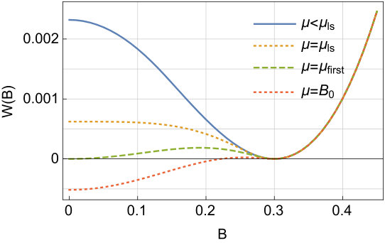 Figure 1
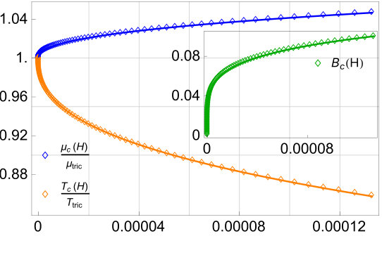 Figure 2
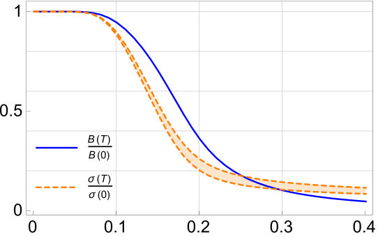 Figure 3
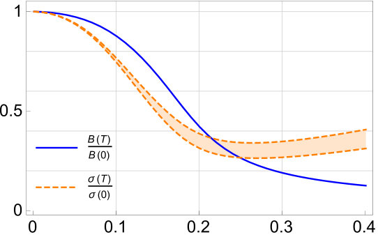 Figure 4
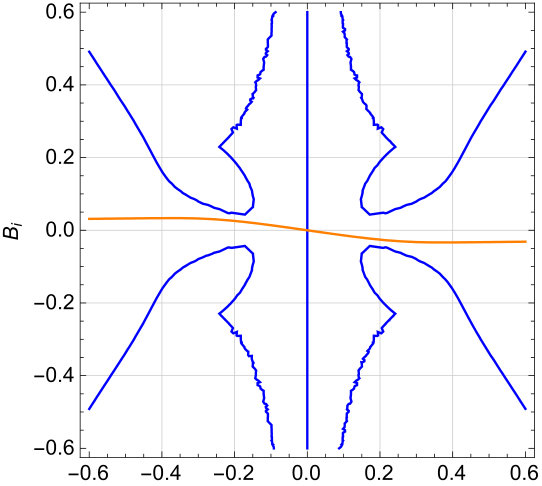 Figure 5
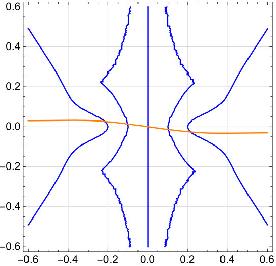 Figure 6
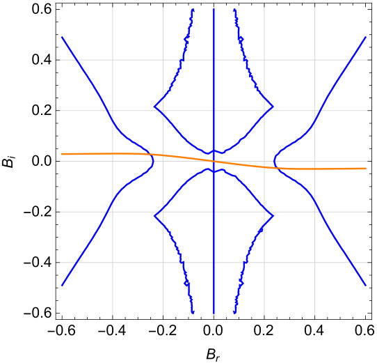 Figure 7
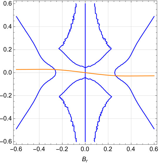 Figure 8
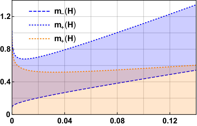 Figure 9
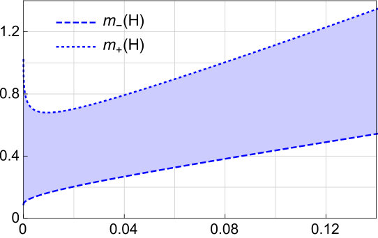 Figure 10
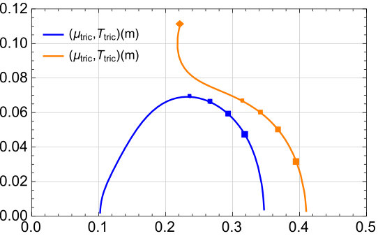 Figure 11
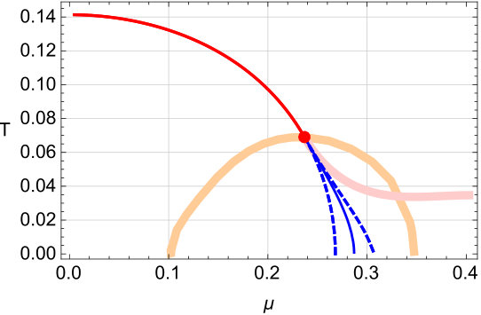 Figure 12
| Chiral limit () | ||||||
|---|---|---|---|---|---|---|
| Physical localization | 237 | 69 | 141 | 268 | 287 | 305 |
| Euclidean localization | 318 | 64 | 150 | 346 | 365 | 376 |
| Jakovac et al. Jakovac:2003ar | 280 | 60 | 140 | |||
| Schaefer et al. Schaefer:2004en | 251 | 52 | 142 | |||
| Hatta et al. Hatta:2002sj | 209 | 107 | – | |||
| Qin et al. Qin:2010nq A | 140 | 110 | 124 | |||
| Qin et al. Qin:2010nq B | 130 | 120 | 133 | |||
| Costa et al. Costa:2008yh | 286 | 112 | 215 |
| Models for CEP | ||
|---|---|---|
| Physical localization | 389 | 35 |
| Euclidean localization | 427 | 22 |
| Hatta et al. Hatta:2002sj | 279 | 95 |
| Ayala et al. Ayala:2017ucc | 315-349 | 18-45 |
| Cui et al. Cui:2017ilj | 245 | 38 |
| Yokota et al. Yokota:2016ovb | 287 | 5 |
| Contrera et al. Contrera:2016rqj | 319 | 70 |
| Knaute et al. Knaute:2017opk | 204 | 112 |
| Antoniou et al. Antoniou:2017vti | 256 | 150 |
| Scavenius et al. Scavenius:2000qd LM | 207 | 99 |
| Scavenius et al. Scavenius:2000qd NJL | 332 | 46 |
| Fischer et al. Fischer:2014ata | 168 | 115 |
| Tripolt et al. Tripolt:2014wra | 293 | 10 |
| Costa et al. Costa:2008yh | 332 | 80 |
| Kovacs et al. Kovacs:2007sy | 320 | 63 |
Peer Reviews
No public reviews on file for this paper yet. If you reviewed it on a platform where reviews are public (OpenReview, ICLR, NeurIPS, ICML), you can paste yours below so the community can read it here.
Videos
No videos yet. Explain this paper in a talk, walkthrough, or lecture? Add one.
Localized rainbows in the QCD phase diagram
J. Maelger
Centre de Physique Théorique (CPHT), CNRS, Ecole Polytechnique, Institut Polytechnique de Paris,
Route de Saclay, F-91128 Palaiseau, France.
Astro-Particule et Cosmologie (APC), CNRS UMR 7164, Université Paris Diderot,
10, rue Alice Domon et Léonie Duquet, 75205 Paris Cedex 13, France.
U. Reinosa
Centre de Physique Théorique (CPHT), CNRS, Ecole Polytechnique, Institut Polytechnique de Paris,
Route de Saclay, F-91128 Palaiseau, France.
J. Serreau
Astro-Particule et Cosmologie (APC), CNRS UMR 7164, Université Paris Diderot,
10, rue Alice Domon et Léonie Duquet, 75205 Paris Cedex 13, France.
Abstract
We study the phase diagram of strongly interacting matter with light quarks using a recently proposed, small parameter approach to infrared QCD in the Landau gauge. This is based on an expansion with respect to both the inverse number of colors and the pure Yang-Mills coupling in the presence of a Curci-Ferrari mass term. At leading order, this leads to the well-known rainbow equation for the quark propagator with a massive gluon propagator. We solve the latter at nonzero temperature and chemical potential using a simple semi-analytic approximation known to capture the essence of chiral symmetry breaking in the vacuum. In the chiral limit, we find a tricritical point which becomes a critical endpoint in the presence of a nonzero bare quark mass, in agreement with the results of nonperturbative functional methods and model calculations. This supports the view that the present approach allows for a systematic study of the QCD phase diagram in a controlled expansion scheme.
I Introduction
Hadronic matter is expected to present a rich phase structure when submitted to sufficiently high energy and baryonic densities, large magnetic fields, etc., as encountered in various environments such as the early universe, ultradense astrophysical objects, or relativistic heavy ion collisions in the laboratory Fukushima:2010bq ; Weissenborn:2011qu ; Borsanyi:2016ksw . Unravelling the phase diagram of quantum chromodynamics (QCD) at nonzero temperature and baryonic chemical potential is a major challenge both experimentally and theoretically. At vanishing chemical potential, first principle lattice simulations unambiguously demonstrate a smooth crossover from a mostly confined to a mostly deconfined phase, accompanied by a restoration of chiral symmetry Aoki:2006br ; Bazavov:2011nk . The crossover region sharpens for increasing quark masses and turns in a second order phase transition for critical values of the quarks masses, above which the transition is first order. The same is expected to happen with the chiral transition in the opposite limit of decreasing quark masses: the transition turns first order below a critical value of the quark masses. Although not firmly established by lattice calculations yet DElia:2018fjp , this is the expected behavior of a theory with at least three light quark flavors. The situation with two light quarks is more subtle due to the possible role of the axial anomaly Pisarski:1983ms .
The situation is even less clear at in the low quark mass region (including the physical point), where standard Monte Carlo algorithms are plagued by the infamous sign problem deForcrand:2010ys . The typical expectation is that of a line of first order chiral transition at low temperatures ending at a critical point Stephanov:2004wx . Firmly establishing the existence of the latter and studying its possible experimental signatures has been the topic of intense theoretical work Mohanty:2005mv ; Stephanov:2008qz ; Hatta:2002sj ; Roberts:2000aa ; Fischer:2018sdj ; Fukushima:2013rx ; Ding:2015ona and is among the major physics goals of various present and upcoming experiments Mohanty:2011nm ; Senger:2016wfb ; Ablyazimov:2017guv ; Sakaguchi:2017ggo . Methods to circumvent the sign problem on the lattice have been devised but remain, so far, limited to , and no critical endpoint has been firmly established Fodor:2018wul . To go beyond, a fruitful proposal has been to supplement lattice results for the quenched gluon dynamics with explicit quark contributions by means of nonperturbative functional methods Fischer:2012vc ; Fischer:2013eca ; Eichmann:2015kfa . Existing works neglect the mesonic degrees of freedom—although baryons have been included Eichmann:2015kfa —and find a critical endpoint at a relatively large . A complementary approach uses phenomenological, Nambu-Jona-Lasinio (NJL) or quark-meson models with various degrees of sophistication Jakovac:2003ar ; Schaefer:2007pw ; Fukushima:2008wg ; Herbst:2010rf ; Resch:2017vjs . These typically predict a critical endpoint at relatively large , whose precise location, however, varies significantly from one study to another. One common weakness of such approaches is that the employed approximations lack a systematic ordering principle. One typically explores the whole phase diagram with truncations adjusted against lattice data at , far from the region where a critical point is found.
In the present article, we study this question using a semi-perturbative approach to the infrared dynamics of QCD based on a simple massive extension of the Faddeev-Popov (FP) Lagrangian in the Landau gauge, known as the Curci-Ferrari (CF) model Curci:1976bt ; Tissier:2010ts . In this context, the gluon mass term is motivated both by the results of lattice simulations Bogolubsky:2009dc and by the necessity to modify the FP Lagrangian in the infrared due to Gribov ambiguities Serreau:2012cg . The CF model is the simplest renormalizable deformation of the FP Lagrangian and remains under perturbative control down to the deep infrared: The gluon mass screens the standard perturbative Landau pole and the (running) gauge coupling remains moderate at all scales Tissier:2010ts ; Reinosa:2017qtf , as observed in lattice simulations. A series of recent studies has shown that the perturbative Curci-Ferrari model gives an accurate description of the phase structure of pure Yang-Mills theories and of QCD with heavy quarks Reinosa:2014ooa ; Reinosa:2015oua ; Maelger:2017amh . The case of light quarks is more delicate because, unlike the couplings in the pure gauge sector, the quark-gluon coupling becomes significant in the infrared Skullerud:2003qu . A systematic approximation scheme, nonperturbative in the quark-gluon vertex, has been proposed in Ref. Pelaez:2017bhh , based on a double expansion in powers of the pure gauge coupling and of the inverse number of colors . At leading order, this leads to the well-known rainbow equation and, therefore, successfully describes the dynamics of chiral symmetry breaking in the vacuum. There are however too notable differences with respect to the usual implementations of the rainbow equation: first, the gluon exchange is described in terms of a tree-level Curci-Ferrari propagator, and second, higher order corrections are controlled by small parameters, which allows in particular to include renormalization group effects in a consistent way Pelaez:2017bhh .
The purpose of the present work is to extend this approach to nonzero temperature and nonzero chemical potential, paving the way for a systematic study of the predictions of the CF model for the QCD phase diagram.
II The rainbow equation in the Curci-Ferrari model
For simplicity, we study a theory with degenerate quark flavors. At nonzero temperature and quark chemical potential , the rainbow equation for the (Euclidean) quark propagator reads
[TABLE]
where and denote the bare quark mass and quark-gluon coupling, respectively. We have introduced Euclidean momenta , and , with and () the bosonic and fermionic Matsubara frequencies respectively. Correspondingly, the bosonic and fermionic Matsubara sums will be denoted
[TABLE]
where it is implicitly understood that integrals over the norm of three-dimensional momenta are cut off at a scale . The matrices stand for the Euclidean Dirac matrices, with , which we choose in the Weyl basis, such that and . Finally, the tree-level gluon propagator is
[TABLE]
with the transverse projector and the Curci-Ferrari mass.
In Appendix A, see also Roberts:2000aa , we recall that the quark propagator decomposes as (we keep the -dependence explicit)
[TABLE]
with any of the components or depending on only through its norm and such that
[TABLE]
These considerations apply also to the inverse propagator which we parametrize as
[TABLE]
We have , with
[TABLE]
Projecting Eq. (1) onto the various tensor components, one arrives at a non-linear system of integral equations:
[TABLE]
where , and , as well as . We have also introduced the quadratic Casimir in the fundamental representation .
In the chiral limit, corresponding to , an unbroken chiral symmetry implies , which obviously solve the (homogeneous) equations (10) and (13). This also means that a solution with either or signals the spontanous breaking of chiral symmetry. In what follows, we use as our order parameter for chiral symmetry breaking since remains an allowed solution (which we stick to) also away from the chiral limit. In order to keep the discussion as simple as possible, we also set the other functions to their tree-level values, , .
With this ansatz, the rainbow equation for the quark mass function , Eq. (10), reads
[TABLE]
where we have defined and we recall that, in the case of a real chemical potential,
[TABLE]
as follows from Eqs. (6) and (7). In particular, is real for but becomes a priori complex when is non-zero.111An interesting exception that we shall exploit below is the zero-temperature limit for fixed integer in . In this limit, and becomes real. We mention that it is also real in the case of an imaginary chemical potential.
III Localization
In this article, we analyse the solutions to Eq. (II) by using an approximation scheme called localization Reinosa:2011cs ; Marko:2015gpa , which we now recall and extend to the problem at hand.
In a given model, the value of the mass function at a given momentum depends on the value of the mass function at any other momentum. However, there can be cases where, in some range of parameters and to a reasonable level of accuracy, the value of the mass function at a particular scale decouples from the rest and obeys, therefore, a simpler, “localized” equation. For instance, in Ref. Reinosa:2011cs , the behavior of the mass function at zero momentum was essentially controlled by the zero-momentum mass itself. The self-consistent equation for this zero-momentum mode could be obtained by expanding the mass function about this zero-momentum value in the corresponding integrals.
Even in cases where there is not a clear argument of why a certain scale could decouple, the localized equations often provide a good qualitative guide. In the present case, it correctly captures the phenomenology of chiral symmetry breaking in the vacuum.
Of course, rainbow equations similar to Eq. (II) have been solved before without the need to resort to localization, even at finite temperature. Localization is however a convenient approach that could be used as a first investigation of more intricate settings such as the rainbow equation in the presence of non-trivial gluonic background (accounting for the interplay between chiral and center symmetry), or the corrections beyond the rainbow approximation, within the systematic expansion scheme alluded to in the Introduction.
One of the goals of this work is to investigate this strategy in a simpler setting before applying it to these more complicated cases. In order to test the robustness of the approach, we shall consider two types of localizations, referred to below as Euclidean and physical respectively, and which we now define more precisely.
III.1 Euclidean localization
At finite temperature, it is important to stress that the Euclidean mass function is defined a priori on the fermionic Matsubara frequencies, which never vanish. We shall therefore localize the mass function at the smallest momentum available, that is, . Since , it is natural – and in fact crucial, as we illustrate below – to localize together with . This means that we should consider two regions in the integrals, the one where it makes sense to expand the mass function about and the one where it makes sense to expand it about . Therefore, we approximate (II), with or by
[TABLE]
and
[TABLE]
which are easily checked to be compatible with . It is convenient to work with the real quantities
[TABLE]
In terms of and , the rainbow equations for read
[TABLE]
and
[TABLE]
After performing the Matsubara sums and the angular integrals, Eqs. (20)-(21) rewrite in the simple form
[TABLE]
where, for notational convenience, we have defined
[TABLE]
with
[TABLE]
with and where denote the Bose-Einstein and Fermi-Dirac distributions. We note that is not the complex conjugate of , due to the dependence on which we leave, however, implicit in what follows.
III.2 Physical localization
One inconvenient aspect of the Euclidean localization is that one has to deal with two variables, and . This prevents the definition of a potential associated to the localized equations, due to the fact that the latter do not comply with the Cauchy-Riemann conditions. Although many features of the phase diagram do not require the existence of an underlying potential, it is convenient to find a setting where one deals with only one variable instead of two.222We will see below that, after renormalization, there is one particular way to achieve this within the Euclidean localization. There are also certain limits, such as or , where this becomes possible due to the fact that . Another drawback of the Euclidean localization is that it involves the first Matsubara frequency . Therefore, we expect its quality to decrease as the temperature is increased.
One way to try to cope with these limitations is to consider a localization based on the retarded mass function
[TABLE]
evaluated for and . The reason for the presence of in the prescription to obtain the physical retarded Green’s function is recalled in Appendix B, see also Ref. Laine:2016hma . We find that, for real and smaller than , the corresponding analytic continuation of in Eq. (24) is real in the limit .333One should pay attention to the fact that what is really continued are not and , but rather . Therefore, the equation for becomes compatible with the solution , which we assume from now on, and the equation for reduces down to
[TABLE]
where is to be evaluated with and in the energy denominators. While remains the same as above, we now have
[TABLE]
One price to pay for this choice of localization is the singularity at , which is regulated in the retarded self-energy through . We ignore this issue and restrict our analysis to cases where . This is justified both because the physically relevant values in the vacuum fall in this range (see below) and because most of our discussions below concern the vicinity of the symmetric point .444On the other hand, the constraint does not allow for a smooth continuation from the chiral limit to the heavy quark limit since is always constrained to be less than . This is one of the reasons why we also develop the Euclidean localization. We note finally that, interestingly (although not surprisingly), the localized equation (28) reduces to the corresponding mean-field gap equation of a NJL-type model with an effective nonlocal four-fermion vertex corresponding to a massive gluon exchange.
IV Results
We now investigate our predictions for the phase diagram using the two types of localizations, starting with the physical localization.
IV.1 Physical localization
Consider first the chiral limit, corresponding to . For large enough values of the coupling, Eq. (28) admits nontrivial, symmetry breaking solutions on top of the chirally symmetric solution . It is convenient to parametrize the equation in terms of the dynamical mass in the vacuum, , given by
[TABLE]
where we see that symmetry-breaking solutions exist only if . We use Eq. (30) to trade the bare quark-gluon coupling for the (ultraviolet finite) quark mass . The rainbow equation rewrites as
[TABLE]
where we note that the cut-off can now be sent to infinity:
[TABLE]
It is useful to interpret Eq. (31) as deriving from a chirally symmetric potential , with , that is . The absolute minima of then determine the state of the system. At , one easily checks that the nontrivial minimum, equal to in the vacuum, decreases with increasing temperature and continuously reaches at a critical temperature. This extends in a critical line of second-order phase transitions in the plane, defined by the condition , as shown in Fig. 1. Depending on the parameters, this critical line can turn into a line of first-order transitions at a tricritical point, defined by the conditions for or, equivalently,
[TABLE]
The first-order line is then determined from
[TABLE]
where is the nontrivial minimum at the transition. The associated lower and upper spinodals are respectively defined by
[TABLE]
with the location of the nontrivial metastable state at the upper spinodal. The two spinodals flank the first order line and merge at the tricritical point, beyond which the lower spinodal becomes the critical line. The equation governing the critical and lower spinodal lines is easily obtained as
[TABLE]
which is a strictly concave line. For low enough temperatures , the gluonic thermal contribution (second term) in Eq. (36) is negligible and one obtains the approximate expression
[TABLE]
This is similar to the result obtained in the quark-meson model with a large- approximation Jakovac:2003ar .
We note that there is an ambiguity in the definition of the potential since neither the solutions of Eq. (31) nor their convexity are altered by the replacement with a differentiable and strictly positive function. Interestingly, because the conditions (33) and (35) only involve and its derivatives, they are, in fact, independent of the function and so are, thus, the spinodal lines, the line of second-order transition, and, of course, the tricritical point where these lines meet. Only the line of first-order transition explicitly depends on through the second condition in Eq. (34). However, it always lies in between the two spinodals.
In Fig. 1, we show our results for the phase diagram in the chiral limit. We use the typical values MeV and MeV, motivated by the study of dynamical chiral symmetry breaking in the Curci-Ferrari model in the vacuum Pelaez:2017bhh . We find a tricritical point located at . The transition at zero chemical potential occurs at MeV and the two spinodals meet the axis for MeV, and MeV, respectively. This gives an estimate of the first-order transition line at most at the 10% level, independently of the function (the estimate improves as one approaches the tricritical point). For the choice , the transition point is at MeV.
In fact, Eq. (31) greatly simplifies at , where
[TABLE]
if and otherwise. In particular, we see that the value of the order parameter below the transition point is independent of , , until it jumps to in the symmetric phase. This is known as the Silver Blaze property Cohen:2003kd ; Marko:2014hea , which we illustrate in Fig. 2.555We mention that the Silver Blaze property should in princple extend only up to the the first singularity on the axis, namely the nuclear liquid-gas transition. Here, however, our level of description does not capture the corresponding dynamics, and the Silver Blaze property extends further. We also mention that the -independence below the first singularity applies in principle only to [math]-point functions. For higher -point functions, it takes a more general form as shown in Marko:2014hea . However, due to the presence of in the retarded prescription (27), it can be argued that the Silver-Blaze property applies to retarded Green functions as it does for [math]-point functions. Also, using Eqs. (32) and (38), we can determine the values of the gluon mass for which there exists a tricritical point. The latter reaches the axis for some values of the ratio . Defining , we get the condition , which has two solutions in , , with . One finds and . The corresponding values of are given by Eq. (36) at , , yielding and . There exists a tricritical point iff as shown in Fig. 1.
Let us now move away from the chiral limit. Equation (31) now reads , where needs to be seen as a finite parameter controlling the departure from the chiral limit. For , the second-order transitions turn into crossovers and the tricritical point becomes a critical endpoint terminating a first-order line. Writing the potential , the conditions for a critical point are
[TABLE]
from which one extracts , , and for each . To this aim, it is convenient to vary , determine and from the last two conditions in Eq. (39)—that do not involve —and then deduce from the first condition. Inverting this relation, one then gains access to and . In particular, we find that the approach to tricriticality is governed by mean field exponents; see Fig. 3. This is expected because the potential is regular around . The trajectory of the critical endpoint in the phase diagram, shown in Fig. 1, exhibits a nonmonotonous behavior of as a function of , similar to that observed in Ref. Hatta:2002sj using an approach based on the Cornwall-Jackiw-Tomboulis effective potential. Finally, Fig. 4 shows the interval compatible with a critical point for each value of . Interestingly, in the physical localization considered here, the Curci-Ferrari mass should be neither too large nor too small for a critical end point to exist.
IV.2 Euclidean localization
Let us now investigate the Euclidean localization, that allows us to test the robustness of the previous features.
To renormalize the equations in this case, we proceed as follows. First, we note that the function possesses a logarithmic UV divergence which however does not depend on . It is then readily checked that the equation for has a divergence proportional to . This divergence can be absorbed into a redefinition of the bare coupling as follows. We divide the corresponding equation by and set
[TABLE]
where the renormalized coupling should be interpreted as being defined at the (real) renormalization scale . Introducing as before, the renormalized equation for takes the form
[TABLE]
with .
As far as the equation for is concerned, it is easily checked that it is finite, for any fixed . Therefore, using the redefinition (40) or the bare coupling is problematic here since it leads to a spurious cut-off dependence. This problem is rooted in the localization procedure which does not commute with the renormalization procedure, see Marko:2015gpa for more details. However, we can always define a renormalized localized scheme by replacing by in the equation for :
[TABLE]
We note that, in this equation, one can interchangeably use or .
With this choice of renormalization, we can eventually express the equations in terms of the vacuum mass in the chiral limit, , see Eq. (30). It is related to and by
[TABLE]
Replacing in that form, one checks that the first term in the RHS of (41) disappears while the scale in is replaced by . Thus, Eq. (41) does not depend on . However a scale dependence remains in equation (42), as expected at a given order of approximation. Below, we shall test the dependence of our results on the renormalization scale .
Let us also mention that, because of the localization procedure, the coupled gap equations (41) and (42), which we denote formally as and in what follows, cannot be seen as deriving from a potential, because, in general the Cauchy-Riemann condition is not satisfied. However, certain features of the phase diagram can be defined without the need of a potential because they correspond to the merging of different solutions of the gap equations. For instance, suppose that we want to investigate whether becomes critical. To this purpose, we solve for as a function of from its gap equation:
[TABLE]
and construct a potential for by integrating
[TABLE]
In the chiral limit, the criticality condition reads . Simple algebra using (44) and (45) leads to the condition
[TABLE]
Now, it is easily verified that , from which it follows that . Similarly, writing , we have and therefore . From these remarks, it follows that the condition for a critical point in the chiral limit simplifies to
[TABLE]
The same equation defines the lower spinodal in the case of a first order phase transition. The upper spinodal is also determined from (46) but without evaluating it for and coupling it to the gap equation for . Finally, the tricritical point is determined from conditions . We find
[TABLE]
where the indices , , and take the values or , and . We have again made use of . This formula simplifies further because . We note however that we are not able to fully eliminate , contrary to what happened for the critical point [see below for a particular limit where this becomes possible].
Our results in the chiral limit (with GeV) are summarized in Table 1 and compared to the results in the physical localization as well as to the results in other approaches. The last column shows the values of at which the lower and upper spinodals ( and ) and the first order transition () are reached for . As already discussed in the previous section, the value of has the largest uncertainty since it depends on the potential which is not uniquely defined in our approach. Also, it may look surprising that we could obtain a value in the Euclidean localization case since there is no potential in this case compatible with the gap equations. However, in the limit, it is readily checked using (15) that vanishes. We note also that, along the axis, is not constant below the transition. This is of course not in contradiction with the Silver-Blaze property since only [math]-point functions should be constant. The case of the physical localization is a bit peculiar since the retarded prescription (27) with included makes the retarded function behave like a [math]-point function as far as the Silver-Blaze property is concerned.
We mentioned above that it was crucial to localize simultanously in and . Let us illustrate this point here. In Fig. 5, we show the curves and for decreasing temperatures and a large enough chemical potential. The crossings correspond to the various possible solutions in the chiral limit and, because the chemical potential is chosen large enough, we should observe a first order transition pattern. Let us now see how this comes about. The first plot is at a temperature right above the upper spinodal, that is the appearance of a new crossing between the curves and , at which two new extrema are about to appear.666In fact, there are four such extrema since, in the chiral limit, the problem is symmetric under . But it is then enough to restrict to . Below this temperature, the various branches making the curve fuse and reorganize, in such a way that, at an even lower temperature, a second spinodal occurs at where two extrema merge. We observe that the proper realization of this scenario requires not only the various branches to fuse at some temperatures, but also that the number of intersections of the curves and changes from one to five, and then to three, as the temperature is decreased. Had we performed the localization only with respect to , that is by writing only the first term in Eq. (16) and taking the real and imaginary part of the corresponding equation, this second requirement would not be fulfilled, as we have checked explicitly.
Regarding the renormalization scale dependence of our results, we observe numerically that the critical/lower spinodal line does not depend on the scale . This is no surprise since the corresponding equation (46) depends only on which, has we have already argued above is independent. In contrast, the position of the tricritical point along (46), or even the other spinodal emerging from this point do depend on . We note, however, that the inverse coupling diverges positively as the renormalization scale is taken to infinity, see Eq. (43). Since there is no other dependence with respect to in Eq. (42), it follows that should approach [math] in this limit and all relevant features (boundary lines, tri/critical points, …) should converge to a certain limit, obtained by considering a single gap equation (41) in which one sets from the start.777This equation does not become trivial in the limit because, in this case, the -dependence of is cancelled by the corresponding -dependence hidden in . We also mention that the equation obtained in the limit is nothing but the one we would have obtained by applying the naïve renormalization and sending the cut-off to infinity. Indeed the remaining cut-off dependence in the equation for , only present in the term containing , would enforce as . Take for instance the tricritical point. Because in the limit , Eq. (48) becomes
[TABLE]
which is indeed the condition for a tricritical point if one restricts from the beginning to Eq. (41) with .
The relative difference between the tricritical values for GeV and are found to be about a few percent. This indicates a controlled renormalization scale dependence and allows us from now on to work in a simplified picture in the limit. In particular, in this limit, we can associate a potential to the Euclidean localization, such that . We shall now employ this simpler setting to move away from the chiral limit.888We mention that, were we not to consider the simplifying limit , certain properties would remain -independent, such as any property along the or axes. This includes the crossover temperature at or the values for , and for any , as well as the function discussed below.
For a non-zero bare mass, chiral symmetry is explicitly broken. As already mentioned, the second order transition line turns into a crossover and the tricritical point into a critical point. Unlike the critical endpoint, the crossover line has no unique definition. Moreover, there exist as many crossover lines as there are order parameters. In what follows, we define the crossover temperature by the inflection of as a function of the temperature. With this choice, we can determine for which value of the crossover temperature of the quark mass function becomes MeV in the limit of vanishing chemical potential, which is the value found by lattice simulations at the physical point for two flavors Karsch:2000kv . Within our approach, we treat this particular value of to correspond to the “physical point”, . We can determine it conveniently as follows. Denoting by the gap equation in both localization schemes and taking two -derivatives, we have
[TABLE]
Imposing the inflection condition and upon plugging (50) into (IV.2), we arrive at the following condition
[TABLE]
which we can solve for , given the expected crossover temperature. Knowing the crossover value of , we can then determine from the gap equation. For the physical localization, we find MeV whereas for the Euclidean localization, we find MeV. Once is determined, we can then locate the critical point in the associated phase diagram, see Tab. 2.
As can be seen, the community has not yet reached a ballpark consensus on the location of the critical end point in the QCD phase diagram and a wide range of results seem permissible at this point. Our numbers do certainly fall within the group of lower temperatures and larger chemical potentials.
Finally, one can study how our findings for the phase diagram depend on the gluon mass of the Curci-Ferrari model. While MeV is the value that globally works best in both the pure Yang-Mills as well as the unquenched sector, it is nonetheless insightful to vary it as a free parameter. Thereby, for each value of , we always insist on fixing the coupling such that we keep the solution fixed at MeV, in the chiral limit. Away from the chiral limit, we only vary , without further changing .
In Fig. 6, we display the position of the tricritical point in the chiral limit as the Curci-Ferrari mass parameter is varied. As can be seen, the obtained trajectories are qualitatively quite different depending on the considered localization scheme, although for MeV, the tricritical points are not so far apart, in particular in temperature values. Interestingly, while in all localization schemes considered, the gluon mass can never exceed an upper limit , in the Euclidean localization, one might take without losing the tricritical point, so in this case.
As before the definition of is trivially extended to the case of non-zero , where the tricritical point is replaced by a critical end-point. We then show our results for these values in dependence of the symmetry breaking parameter in Fig.7 and in comparison with the findings in the physical localization. Here, we iterate our observation that the existence of a CEP puts an upper bound on the allowed for values for the gluon mass in both localization schemes considered, whereas a lower bound only exists for the physical one.
IV.3 Chiral condensate
As mentioned previously, the mostly used order parameter for the chiral transition is not the constituent quark mass but the chiral condensate. Within the localized schemes considered here, it is natural to approximate the chiral condensate as
[TABLE]
with
[TABLE]
At this level of description, we can adopt an adhoc renormalization of the condensate by removing the divergence in , up to the scale in the logarithm of the vacuum contribution of which makes the renormalized condensate a scale dependent quantity:
[TABLE]
with
[TABLE]
To get some intuition on the behavior of , consider the physically localized gap equation which we rewrite identically as
[TABLE]
In the limit , the tadpole sum-integral grows like , which is only counter-balanced provided vanishes as , in which case we also have . Putting all the pieces together, we find
[TABLE]
and thus
[TABLE]
In the Euclidean localization the condensate is found to grow with at large , which is clearly an artefact.999The coefficient is proportional to however in such a way that the condensate becomes zero in the chiral limit, in the high temperature region. Despite this feature, in both cases, we can define a crossover temperature associated to the inflexion point of the chiral condensate as a function of the temperature. It is found to be lower than the corresponding crossover temperature for . We can also try to fine-tune the value of to bring the crossover temperature for the condensate to the lattice value of MeV. To this purpose, consider the equation . Seeing as a function of and , this equation rewrites
[TABLE]
which we use again to determine the crossover value for , assuming a crossover temperature MeV. The corresponding value of is then obtained from the gap equation. In the physical localization, we find MeV, and a critical end-point located at , but the value of gets suspiciously close to the bound . In the Euclidean localization, it seems not to be possible to reach these transition temperatures, at least at this level of approximation.
V Conclusion
We have computed the phase diagram of QCD with light quarks in the context of a first-principle inspired approach to infrared QCD, the Curci-Ferrari model, using the double expansion in the pure gauge coupling and in proposed in Ref. Pelaez:2017bhh . To allow for a semi-analytic grasp of the corresponding equations and since our first aim is a qualitative survey of what to expect when the equations are solved in full glory, we have used some simplifying approximations, in particular the localization scheme discussed in Reinosa:2011cs ; Marko:2015gpa , which we have extended to the present context. For the parameters used here, the leading-order results agree well with those of effective quark-meson models when the chiral anomaly is neglected Resch:2017vjs ; Jakovac:2003ar . Although subleading in , the latter and meson fluctuations are important to correctly determine the phase structure in the Columbia plot Pisarski:1983ms ; Lenaghan:2000kr ; Resch:2017vjs . In principle, they can be systematically included at next-to-leading order in the present expansion scheme.
We also mention that similar rainbow equations have already been considered in great detail to study the phase diagram in the context of nonperturbative functional approaches Fischer:2012vc ; Hatta:2002sj . Not too surprisingly, our results agree qualitatively with those (the main differences may be attributed to the different treatments of the gluon sector). However, the key point of the present work is to systematically justify the employed approximation on the basis of identified small parameters in QCD.
Although we used here simplified versions of the complete rainbow equation (1), we expect, inspired by the vacuum case, that our main results are robust. In particular, we have tested that our results do not depend much on the type of localization we use. One notable exception is the fate of the (tri)critical point as the gluon mass is taken to zero. In some scenarios, the existence of a critical end-point seems to require a nonzero gluon mass. It would be interesting to investigate to what extent this is an artefact of the localization procedure by solving the original equation (II). Another, obvious extension of the present work will be to include the other scalar functions , , and in Eq. (1), see Refs. Roberts:2000aa ; Fischer:2018sdj .
Yet another interesting direction of investigation is to include the order parameter of the deconfinement transition, the Polyakov loop, in the spirit of Refs. Reinosa:2014ooa ; Reinosa:2015oua ; Maelger:2017amh , which would allow one to study the interplay between the chiral and deconfinement phase transition across the Columbia plot Fukushima:2003fw ; Schaefer:2007pw ; Folkestad:2018psc .
Acknowledgements.
We thank Zs. Szép for interesting discussions and helpful remarks concerning the manuscript.
Appendix A Symmetries of the quark propagator
The full propagator is a function of the external momentum variables and as well as and . Dropping the explicit -dependence for notational simplicity, and assuming isotropy, its tensor structure can decomposed as
[TABLE]
where , and . Under a parity transformation
[TABLE]
and thus parity invariance implies . In fact, in what follows, it is convenient to use the parametrisation
[TABLE]
Under charge conjugation
[TABLE]
where we have used , valid in the particular (Weyl) representation of the matrices considered here. Charge conjugation invariance then implies
[TABLE]
for any of the components . Similarly, under complex conjugation
[TABLE]
where we have used , valid, again, in the Weyl representation. It follows that
[TABLE]
for any of the components . Combining (65) and (67), we also obtain
[TABLE]
In particular, all components are real in the case of an imaginary chemical potential. In the case of a real chemical potential, these components become complex, the real and imaginary parts, corresponding to the frequency even and odd parts, and , respectively.
Appendix B Retarded Green’s function at finite
We briefly recall the origin of Eq. (27), considering, for simplicity, the case of a charged scalar field. The physical retarded propagator is defined as
[TABLE]
where denotes the grand-canonical partition function, and is the Heisenberg field, evolving according to and not . Let us note that we use an unconventional sign for the chemical potential (to be consistent with our choice in Reinosa:2015oua ; Maelger:2017amh ) while keeping the usual convention for the charge, such that and .
Now, we would like to relate the physical retarded propagator to the Matsubara propagator defined as ()
[TABLE]
where now the Heisenberg field evolves in imaginary time, according to , not . The reason for defining the Matsubara propagator in this way is that it possesses a simple functional integral representation.
The relation between the two propagators and is now most easily derived by introducing an auxiliary retarded propagator
[TABLE]
Inserting a complete basis of states under the trace, this relation in Fourier space is found to be
[TABLE]
Moreover, from the commutators of with or , one obtains
[TABLE]
and thus
[TABLE]
Combining (72) and (74), we arrive at the desired result
[TABLE]
The reference list from the paper itself. Each links out to its DOI / PubMed record.
- 1(1) K. Fukushima and T. Hatsuda, Rept. Prog. Phys. 74 (2011) 014001.
- 2(2) S. Weissenborn, I. Sagert, G. Pagliara, M. Hempel and J. Schaffner-Bielich, Astrophys. J. 740 (2011) L 14.
- 3(3) S. Borsányi et al. , Nature (London) 539 (2016) 69.
- 4(4) Y. Aoki, Z. Fodor, S. D. Katz and K. K. Szabo, Phys. Lett. B 643 (2006) 46.
- 5(5) A. Bazavov et al. , Phys. Rev. D 85 (2012) 054503.
- 6(6) M. D’Elia, Nucl. Phys. A 982 (2019) 99.
- 7(7) R. D. Pisarski and F. Wilczek, Phys. Rev. D 29 (1984) 338.
- 8(8) P. de Forcrand, Po S LAT 2009 (2009) 010.