Deep learning for seismic phase detection and picking in the aftershock zone of 2008 Mw7.9 Wenchuan earthquake
Lijun Zhu, Zhigang Peng, James McClellan, Chenyu Li, Dongdong Yao,, Zefeng Li, Lihua Fang

TL;DR
This paper introduces a CNN-based classifier, CPIC, capable of accurately detecting seismic phases in small datasets, significantly improving speed and reliability in aftershock monitoring of the 2008 Wenchuan earthquake and adaptable to other regions.
Contribution
The development of CPIC, a CNN model that maintains high accuracy with limited training data and can be efficiently applied to different seismic regions.
Findings
Detects 97.5% of phases in aftershock data
Maintains over 95% accuracy with only a few thousand training samples
Achieves 97% accuracy after minimal fine-tuning on a different regional dataset
Abstract
The increasing volume of seismic data from long-term continuous monitoring motivates the development of algorithms based on convolutional neural network (CNN) for faster and more reliable phase detection and picking. However, many less studied regions lack a significant amount of labeled events needed for traditional CNN approaches. In this paper, we present a CNN-based Phase- Identification Classifier (CPIC) designed for phase detection and picking on small to medium sized training datasets. When trained on 30,146 labeled phases and applied to one-month of continuous recordings during the aftershock sequences of the 2008 MW 7.9 Wenchuan Earthquake in Sichuan, China, CPIC detects 97.5% of the manually picked phases in the standard catalog and predicts their arrival times with a five-times improvement over the ObsPy AR picker. In addition, unlike other CNN-based approaches that require…
Click any figure to enlarge with its caption.
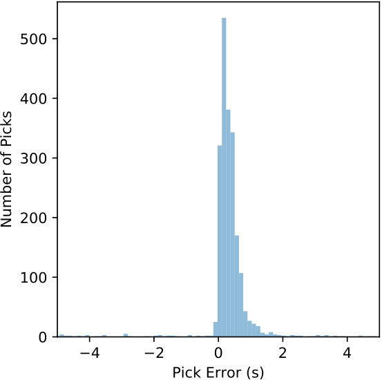 Figure 1
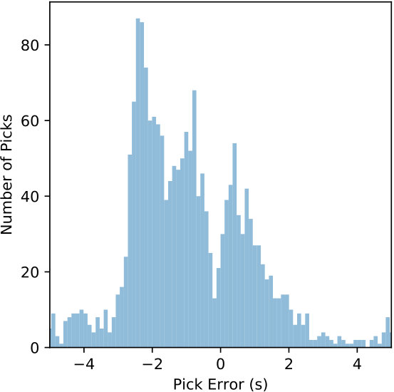 Figure 2
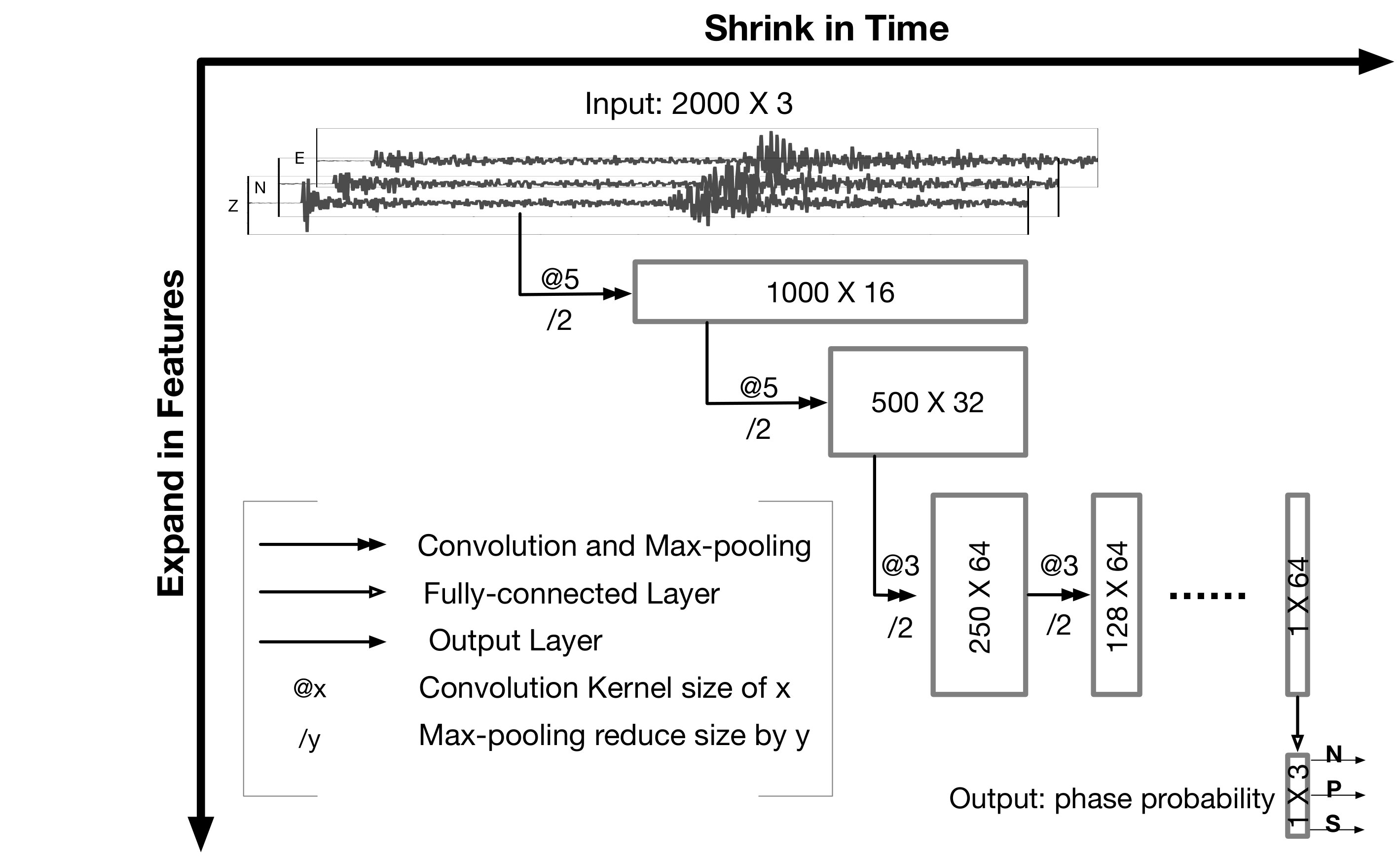 Figure 3
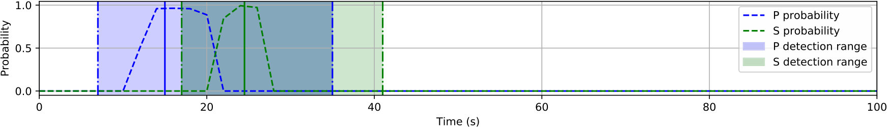 Figure 4
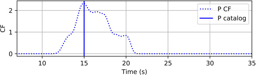 Figure 5
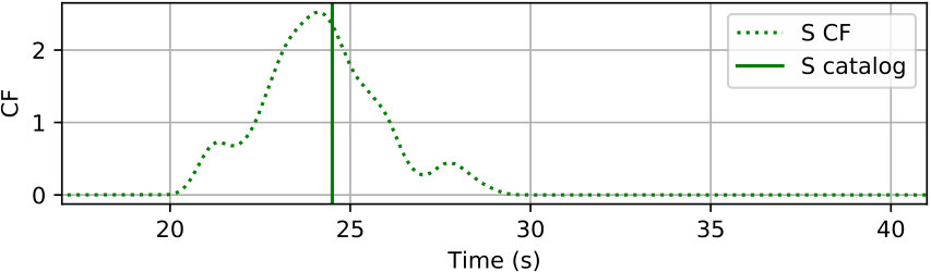 Figure 6
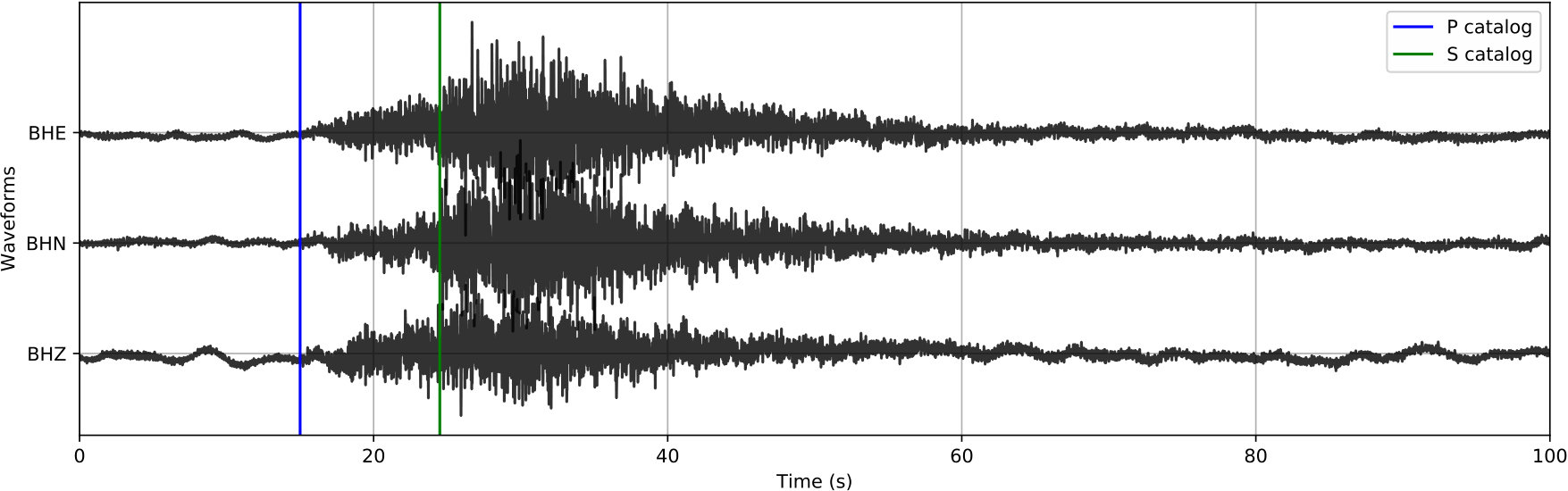 Figure 7
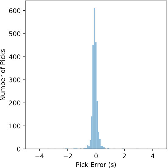 Figure 8
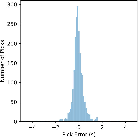 Figure 9
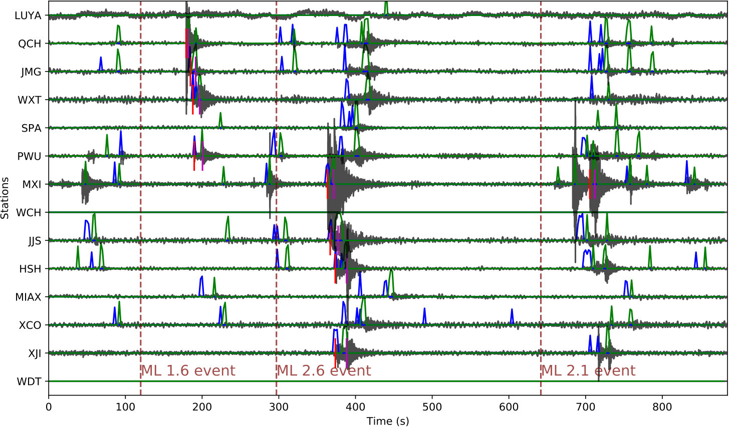 Figure 10
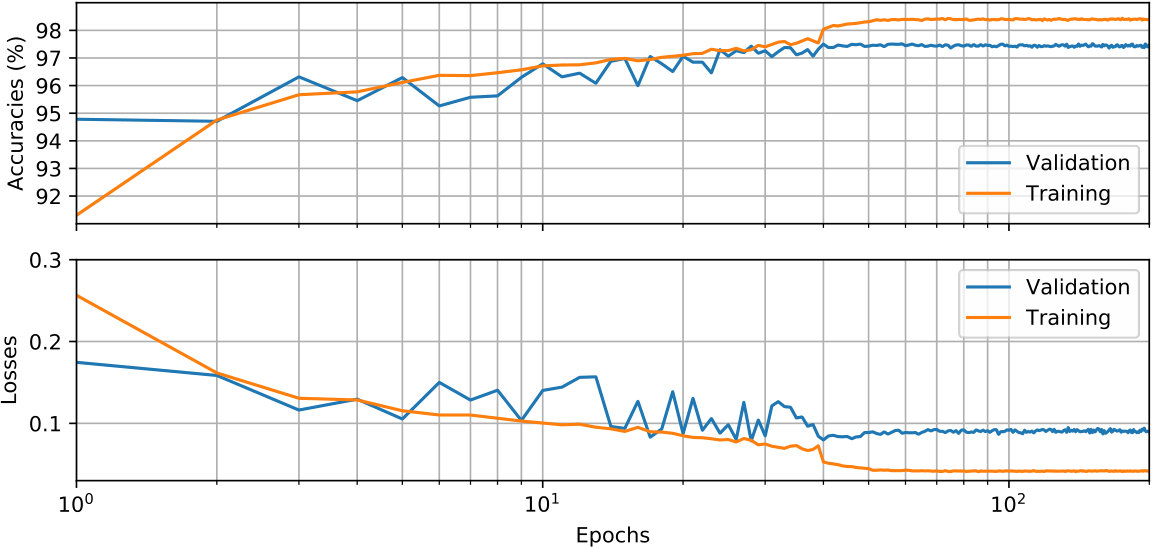 Figure 11
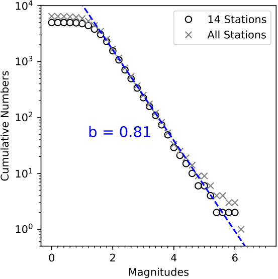 Figure 12
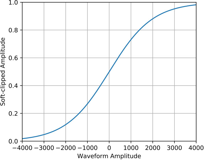 Figure 13
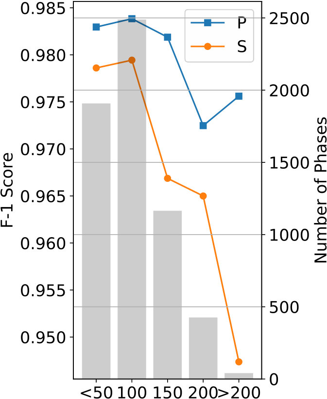 Figure 14
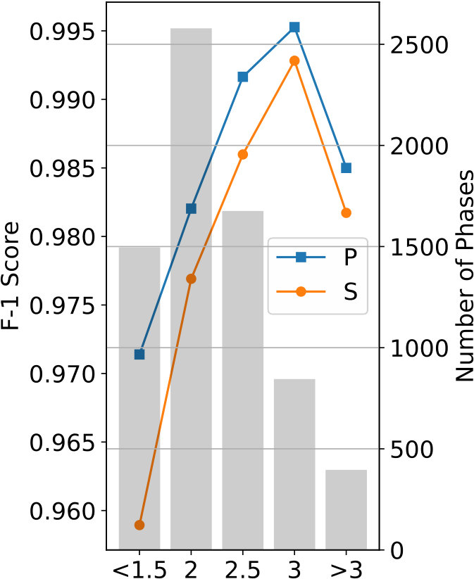 Figure 15
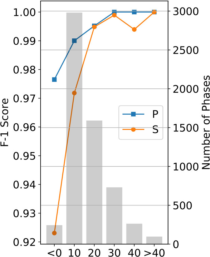 Figure 16
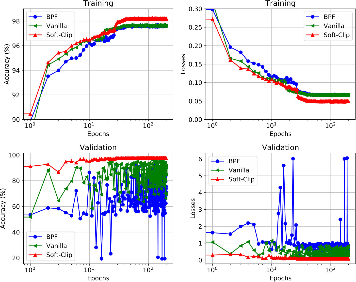 Figure 17
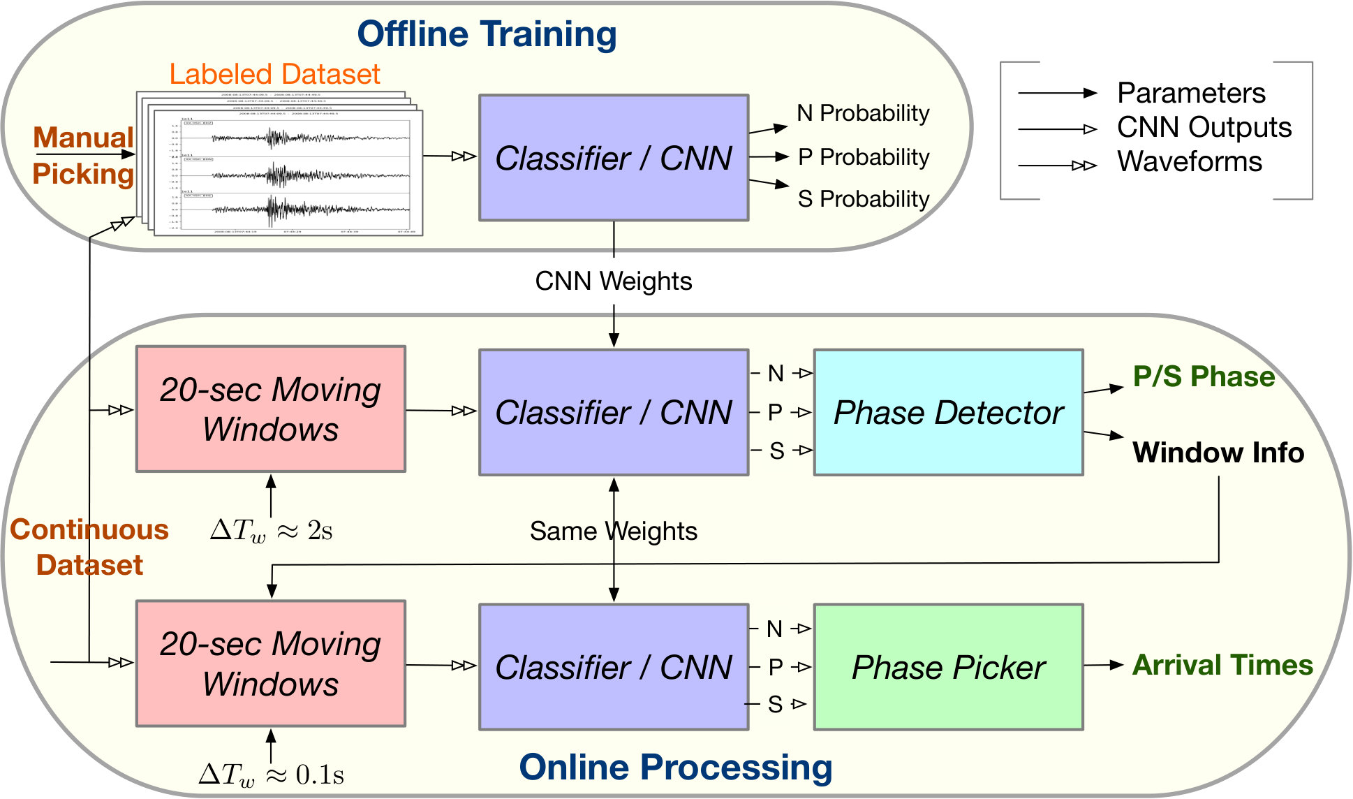 Figure 18
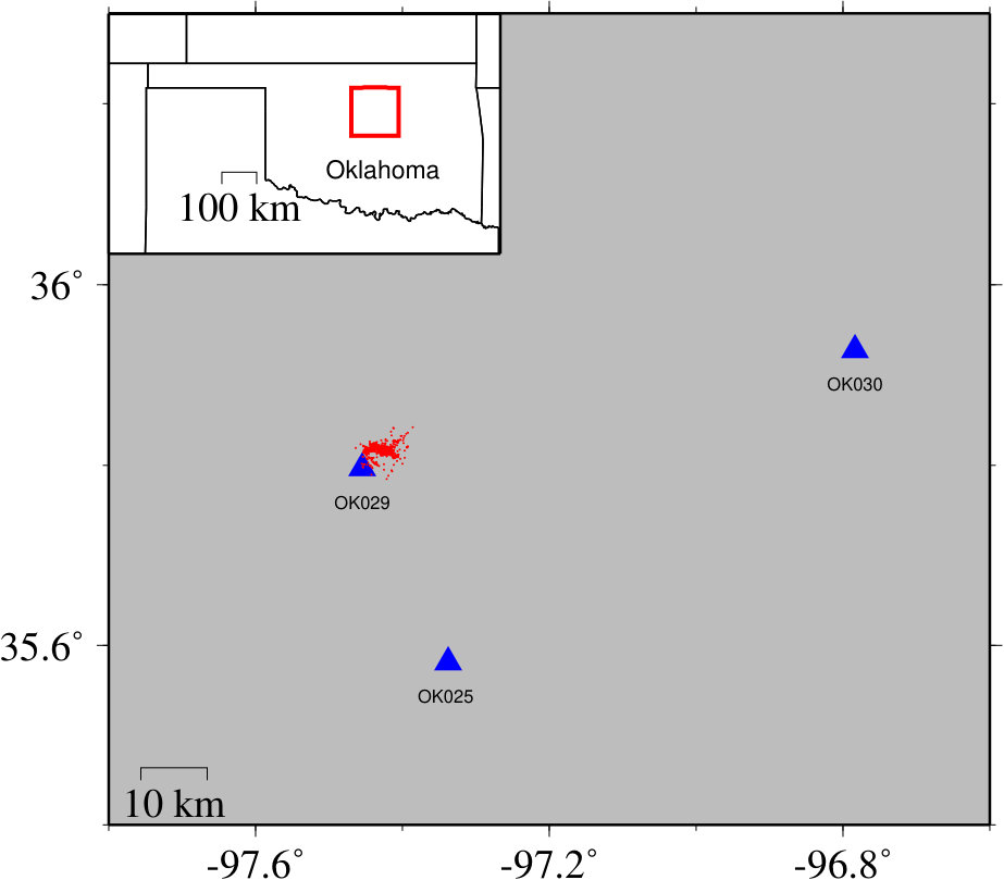 Figure 19
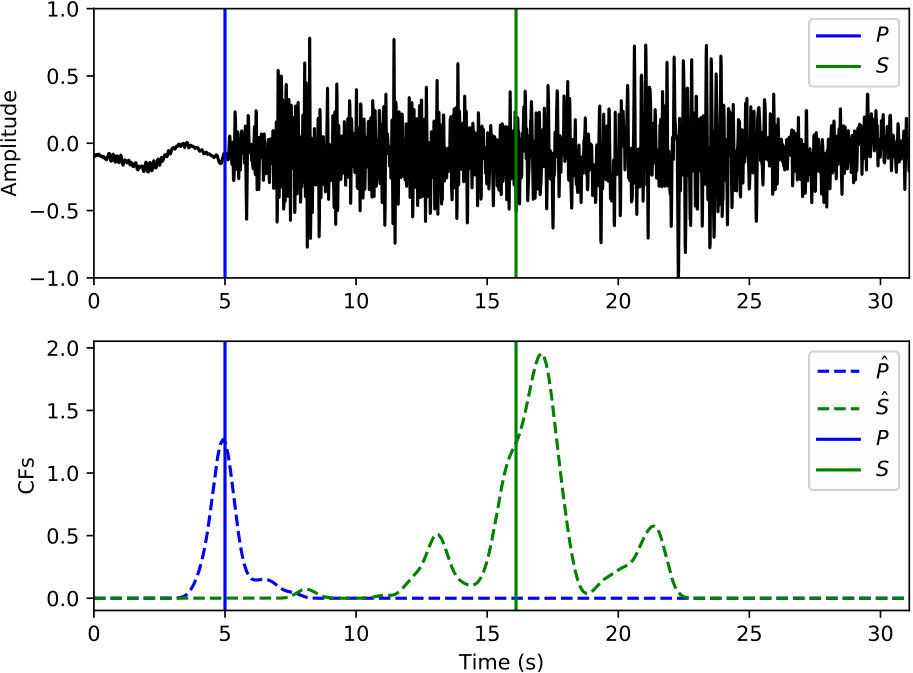 Figure 20
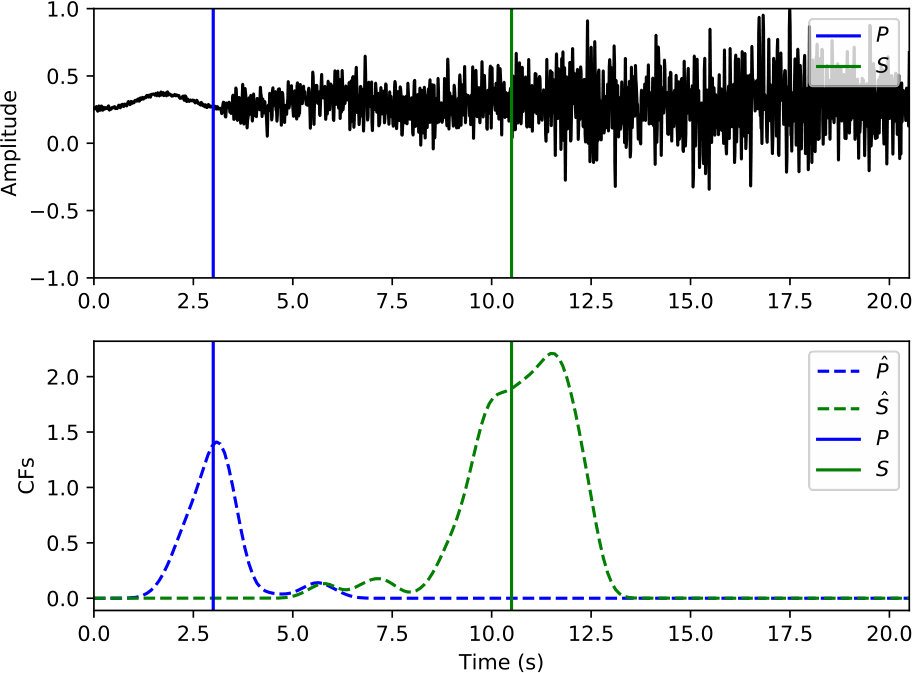 Figure 21
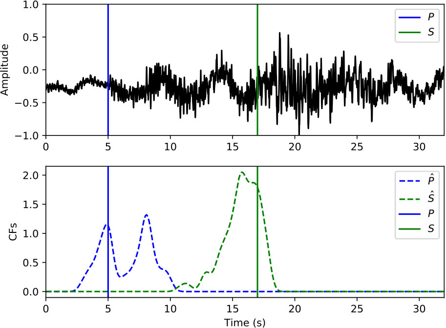 Figure 22
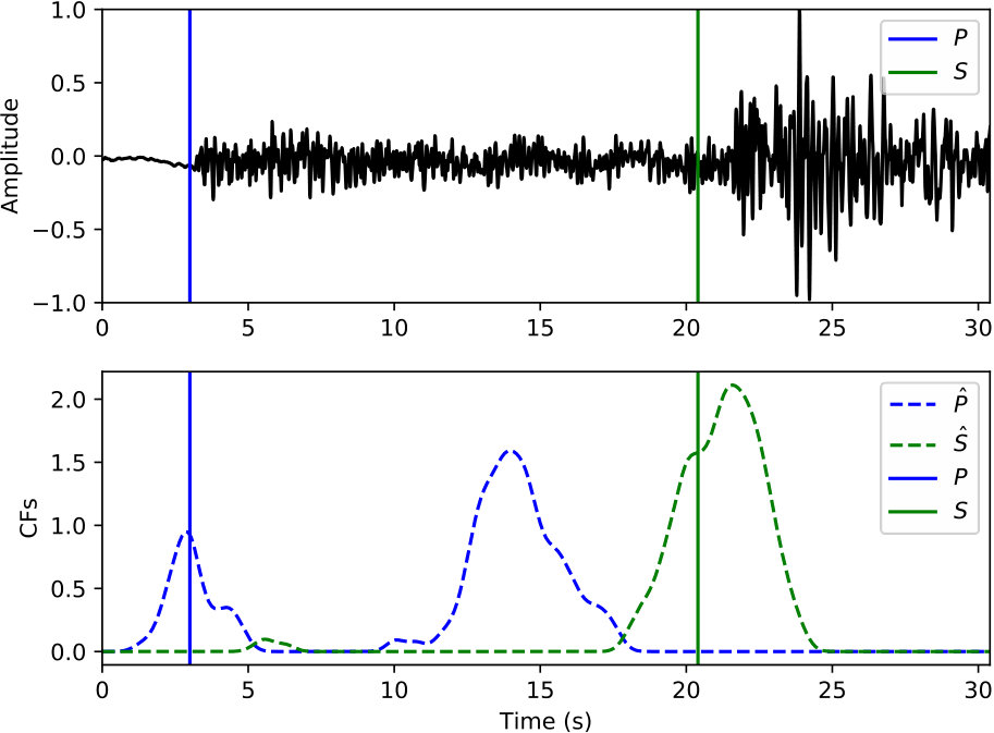 Figure 23
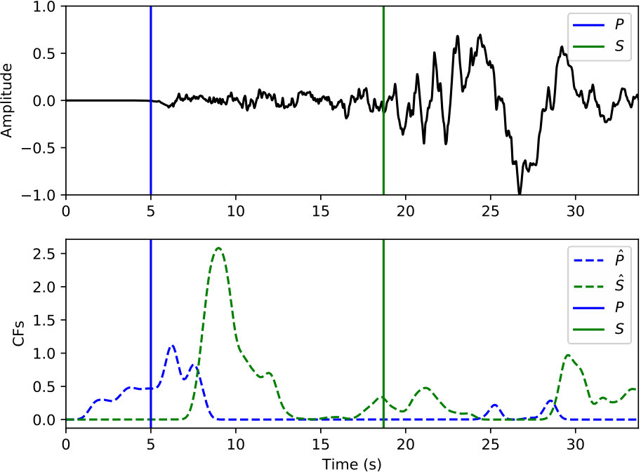 Figure 24
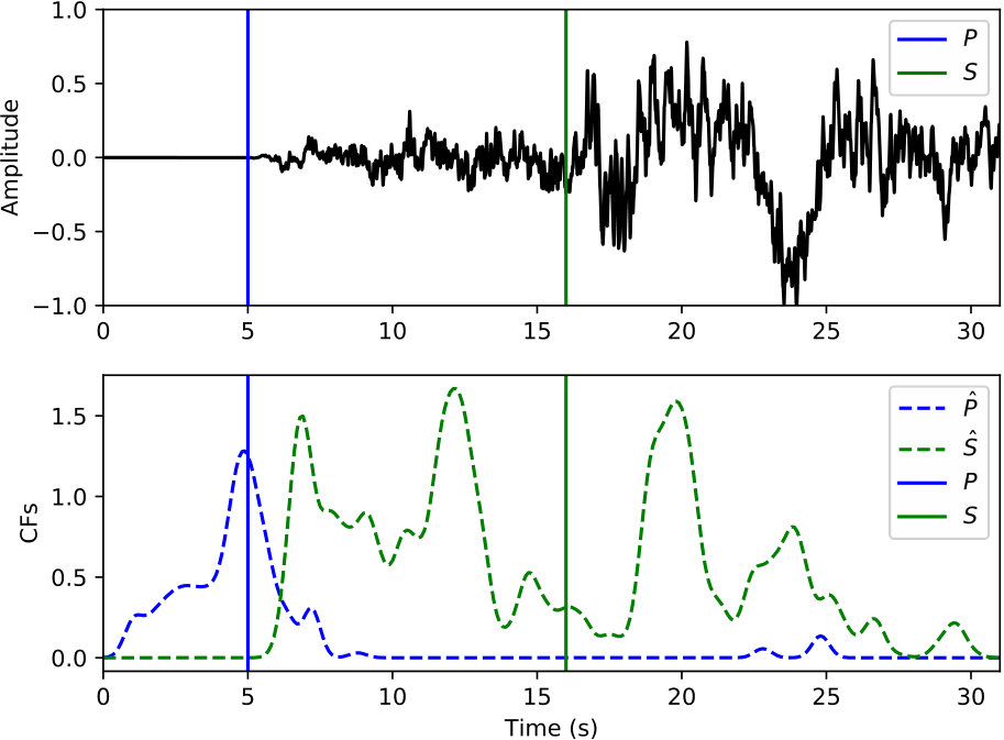 Figure 25
 Figure 26
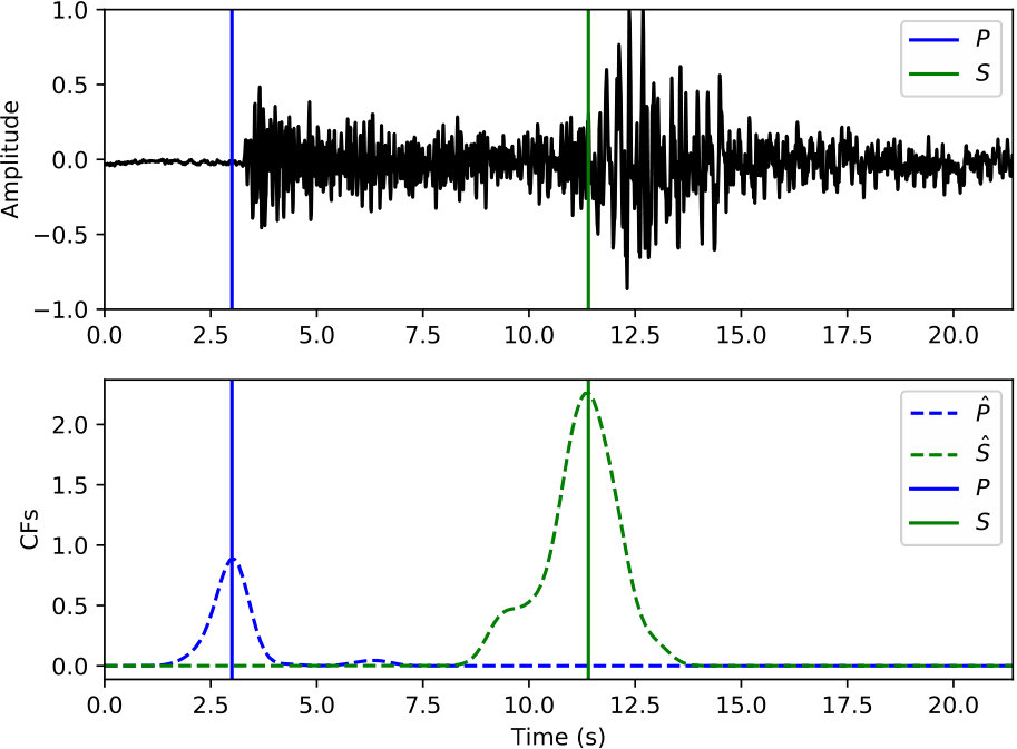 Figure 27
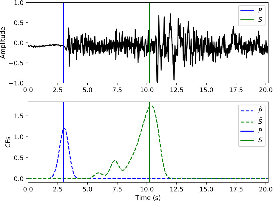 Figure 28
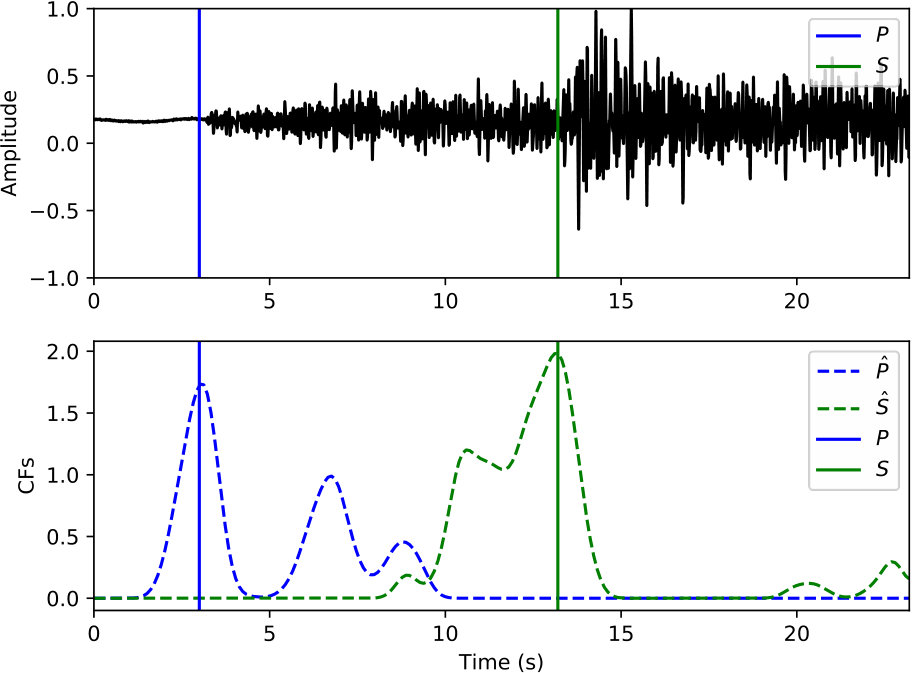 Figure 29
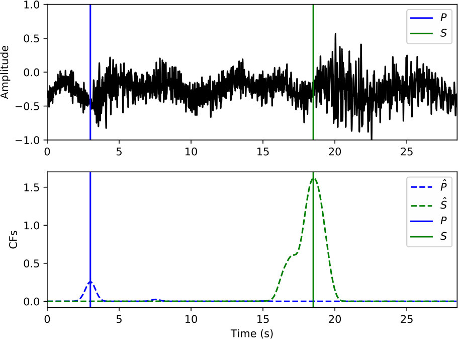 Figure 30
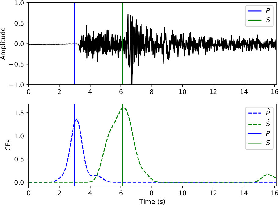 Figure 31
 Figure 32
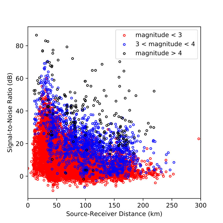 Figure 33
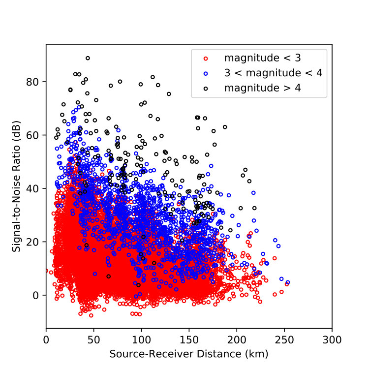 Figure 34
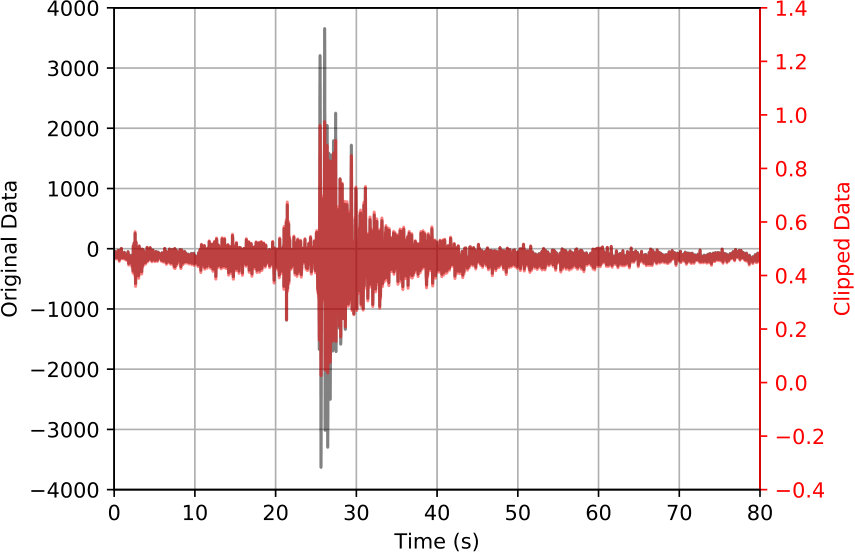 Figure 35
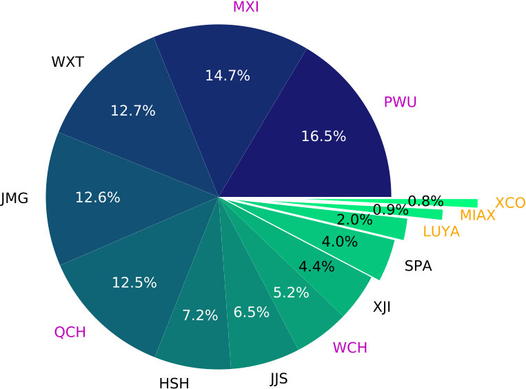 Figure 36
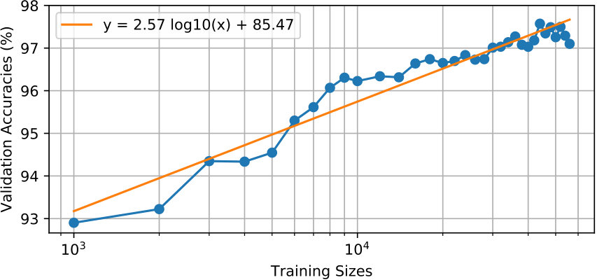 Figure 37
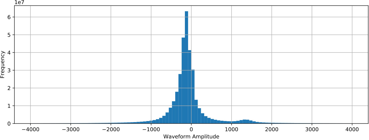 Figure 38
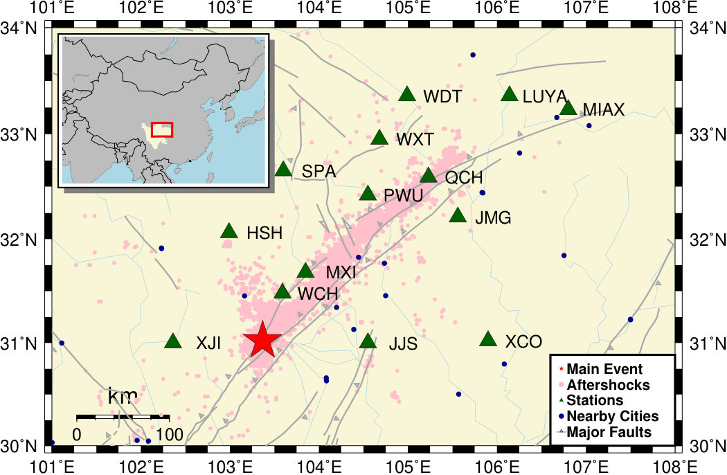 Figure 39
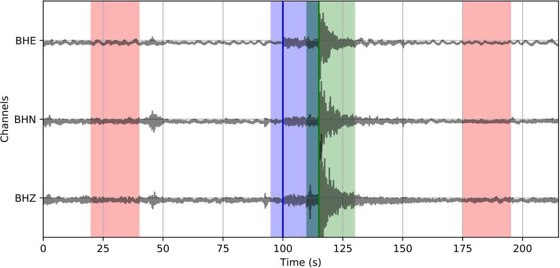 Figure 40
| Detector | |||||
| Noise | P-wave | S-wave | Total | ||
| Catalog | Noise | ||||
| P-wave | |||||
| S-wave | |||||
| Total | |||||
| Detector | |||||
| Noise | P-wave | S-wave | Total | ||
| Catalog | Noise | ||||
| P-wave | |||||
| S-wave | |||||
| Total | |||||
| Categories | Precision | Recall | F-1 Score |
|---|---|---|---|
| Noise | |||
| P-wave | |||
| S-wave |
| Method | ||||
|---|---|---|---|---|
| CPIC picker (ms) | -79.0 | -78.9 | 138.8 | 293.0 |
| ObsPy AR picker (ms) | 311.4 | 936.3 | 671.6 | 1,697.0 |
| Station | OK025 | OK029 | OK030 | All |
|---|---|---|---|---|
| Original (%) | 95.7 | 92.2 | 69.9 | 87.5 |
| Fine-tuned (%) | 98.8 | 96.2 | 94.2 | 97.0 |
| Window Length (sec) | 2.5 | 5 | 10 | 20 | 40 |
|---|---|---|---|---|---|
| Accuracy(%) | 94.7 | 96.3 | 96.9 | 97.4 | 97.2 |
Peer Reviews
No public reviews on file for this paper yet. If you reviewed it on a platform where reviews are public (OpenReview, ICLR, NeurIPS, ICML), you can paste yours below so the community can read it here.
Videos
No videos yet. Explain this paper in a talk, walkthrough, or lecture? Add one.
Deep learning for seismic phase detection and picking in the aftershock zone of 2008 Wenchuan Earthquake
Lijun Zhu
Zhigang Peng
James McClellan
Chenyu Li
DongDong Yao
Zefeng Li
Lihua Fang
School of Electrical and Computer Engineering
Georgia Institute of Technology
Atlanta, GA 30332, U.S.A.
School of Earth and Atmospheric Sciences
Georgia Institute of Technology
Atlanta, GA 30332, U.S.A.
Seismological Laboratory
Division of Geological and Planetary Sciences
California Institute of Technology
Pasadena, CA 91125, U.S.A.
Institute of Geophysics
China Earthquake Administration
Beijing, 100081, China
Abstract
The increasing volume of seismic data from long-term continuous monitoring motivates the development of algorithms based on convolutional neural network (CNN) for faster and more reliable phase detection and picking. However, many less studied regions lack a significant amount of labeled events needed for traditional CNN approaches. In this paper, we present a CNN-based Phase-Identification Classifier (CPIC) designed for phase detection and picking on small to medium sized training datasets. When trained on 30,146 labeled phases and applied to one-month of continuous recordings during the aftershock sequences of the 2008 MW 7.9 Wenchuan Earthquake in Sichuan, China, CPIC detects 97.5% of the manually picked phases in the standard catalog and predicts their arrival times with a five-times improvement over the ObsPy AR picker. In addition, unlike other CNN-based approaches that require millions of training samples, when the off-line training set size of CPIC is reduced to only a few thousand training samples the accuracy stays above 95%. The online implementation of CPIC takes less than 12 hours to pick arrivals in 31-day recordings on 14 stations. In addition to the catalog phases manually picked by analysts, CPIC finds more phases for existing events and new events missed in the catalog. Among those additional detections, some are confirmed by a matched filter method while others require further investigation. Finally, when tested on a small dataset from a different region (Oklahoma, US), CPIC achieves 97% accuracy after fine tuning only the fully connected layer of the model. This result suggests that the CPIC developed in this study can be used to identify and pick P/S arrivals in other regions with no or minimum labeled phases.
keywords:
seismic , detection , phase picking , machine learning , CNN
††journal: Physics of the Earth and Planetary Interiors
1 Introduction
Event detection and phase picking algorithms are becoming increasingly important for automatic processing of large seismic datasets. Reliable automatic methods for P-wave picking have been available for decades. The commonly adopted approaches for automatic picking of seismic phases convert the time-domain signal to a characteristic function (CF), such as short-term/long-term average (STA/LTA) [Allen, 1982], envelope functions [Baer & Kradolfer, 1987], or autoregressive modeling of Akaike Information Criterion (AR-AIC) [Sleeman & van Eck, 1999], and then select the indices of local maxima, or their rising edges, as the picked arrival times. Higher-order statistics, including kurtosis [Saragiotis et al., 2002] and skewness [Nippress et al., 2010, Ross & Ben-Zion, 2014], have also been used to refine the picks due to their sensitivity to abrupt changes in a time series. These algorithms generally perform better for the P waves than S waves, most likely because S-wave arrivals are usually contaminated by the P coda and converted phases. Polarization has been used to discriminate P and S phases [Jurkevics, 1988]. The covariance matrix [Cichowicz, 1993] is used to rotate waveforms into polarized P and S waveform components using methods such as singular value decomposition (SVD) [Rosenberger, 2010, Kurzon et al., 2014]. In general, these existing methods make certain assumptions about the observed seismograms and require careful parameter tweaking when operating on different datasets.
Recently, waveform similarity has been used to detect earthquakes originating from a small region with the same source mechanism while using relatively few parameters [Gibbons & Ringdal, 2006, Shelly et al., 2007, Peng & Zhao, 2009]. A subset of the events with high signal-to-noise ratio (SNR) is manually picked as templates to cross-correlate with continuous waveforms to detect smaller events similar to these templates. The computation cost of such template matching methods scales linearly with respect to the number of templates and dataset size. Since the detected events must be similar to one of the template events, this approach is not as general as the aforementioned STA/LTA. Waveform autocorrelation is one of the most effective methods to detect nearly repeating seismic signals [Brown et al., 2008]. Despite being reliable and robust for different regions, its computation cost scales quadratically with the size of the dataset, making it infeasible when scaled to longer time periods. Further efforts have been devoted to speeding up this process through subspace methods [Harris, 2006, Harris & Dodge, 2011, Barrett & Beroza, 2014], or fingerprint and similarity thresholding (FAST) [Yoon et al., 2015]. Recently, inter-station information has also been considered to improve phase picking efficiency and accuracy through inter-station coherence[Delorey et al., 2017], local similarity [Li et al., 2018] and random sampling [Zhu et al., 2017b].
Facilitated by the parallel computation power of modern graphics processing units (GPUs), deep learning [Goodfellow et al., 2016] took off for speech [Hinton et al., 2012] and image recognition [Krizhevsky et al., 2012] applications. Most deep learning studies share the same fundamental network structure, such as the convolutional neural network (CNN), which further reduces the redundant model complexity of a neural network based on local conjunctions of features from the data (often found in images). Unlike waveform similarity methods, CNNs trained on labeled datasets do not need a growing library of templates and seems to generalize well to waveforms not seen during training. These recent developments have led to CNNs being applied to diverse seismic data sets[Kong et al., 2018], including volcanic events [Luzón et al., 2017], induced seismicity [Perol et al., 2018], aftershocks [Zhu et al., 2018], as well as regular tectonic earthquakes recorded by regional seismic networks [Ross et al., 2018b, a, Zhu & Beroza, 2018]. However, most of these works rely on a large volume of labeled training data which is only available in well-studied regions, such as California, US.
In this study, we accommodate the small seismic datasets by designing a specialized CNN network, named CNN-based Phase-Identification Classifier (CPIC), for single-station multi-channel seismic waveforms. The weights of the CNN are obtained via supervised training based on only thousands of human-labeled phase and non-phase samples used in a recent competition for detecting aftershocks of the 2008 MW 7.9 Wenchuan earthquake in China [Fang et al., 2017]. The CNN learns a compact representation of seismograms in the form of a set of nonlinear local filters. From the training process of discriminating seismic events from noise on large datasets, the weights of the local filters collectively capture the intrinsic features that most effectively represent seismograms for the given task of phase picking. In the next sections, we show that CPIC, trained on a much smaller labeled dataset, achieves comparable classification accuracy as reported in Ross et al. [2018a] and Zhu & Beroza [2018]. CPIC is further tested on a one-month continuous aftershock dataset for phase detection. It achieves accurate detection of manually picked phases, precise arrival times of picked phases, as well as discovering many weak events not listed in the manual-picking catalog.
2 Data
Unlike recent CNN studies that rely on an exceptionally rich training dataset of labeled samples [Zhu & Beroza, 2018, Ross et al., 2018a] to achieve good accuracy and robustness against noise, we design CPIC and study its performance on a relatively small training set prior to applying it on a large volume of unlabeled data. This is a typical scenario when analyzing the aftershock dataset of a major earthquake: strong aftershocks at a later time can be easily picked by existing algorithms or analysts; however, the real targets are the numerous number of aftershocks right after the mainshock that are missed by traditional methods [Kagan, 2004, Peng et al., 2006]. Prior to CNN training and processing, the only pre-processing applied to the seismogram is soft-clipping via a logistic function which is used to normalize the large dynamic range of the input waveforms. As shown in B, such pre-processing contributes to CPIC’s stable convergence as well as higher accuracy. Notably, no filtering is applied to the seismic waveforms in pre-processing.
Study region
We utilize the aftershock dataset of the 2008/05/12 MW 7.9 Wenchuan earthquake that was made available during a recent competition for identifying seismic phases [Fang et al., 2017]. The mainshock occurred on the eastern margin of the Tibetan Plateau (Figure 1), and ruptured the central and northern section of the Longmenshan fault zone [Xu et al., 2009, Feng et al., 2010, Hartzell et al., 2013]. Numerous aftershocks occurred following the mainshock, but many of them were still missing in any published earthquake catalogs [Yin et al., 2018]. The aftershock dataset includes continuous data recorded for one month by 14 permanent stations in August 2008, which is three months after the Wenchuan mainshock. Figure 2(a) shows the distribution of those phases among the 14 stations. Stations near the aftershocks and the rupture zones (e.g., PWU, MXI, WXT, JMG, and QCH) had most of the picked phases, while distant stations (e.g., XCO, MIAX, LUYA, and SPA) have very few; and station WDT has no catalog phase arrivals.
Catalogs
The catalog we used contains 4,986 events with 30,146 phases manually picked on 14 permanent stations with arrivals of P (15,185) of S (14,961) phases. Figure 2(b) shows the catalog events distributed versus magnitude between ML 0.3 to ML 6.2. The signal-to-noise ratio (SNR) of each phase is computed as the ratio of signal powers between two 4-sec waveforms: one after each phase pick (signal) and one before its corresponding P arrival (noise). Figures 2(c) and 2(d) show the distribution of SNR of P and S phases against event magnitudes and source-receiver distance. This catalog was used in a phase picking competition [Zhu et al., 2017a] aiming to improve the detection and picking accuracy from the traditional methods.
Labeled dataset
The CPIC model is trained on a dataset of labeled seismic waveforms in 20-sec long windows. A provides more details. Adding noise-only windows, which are not included in the original labeled dataset, improves CPIC’s trained performance against noisy seismograms. Here, we assume that quiet regions exist between 60 s after an S-wave phase and 60 s before a P-wave phase and generate 30,130 noise-only windows. We note that because those noise windows were not verified manually, it is possible that they may include small aftershocks not listed in the catalog. In the end, we obtain a dataset with 60,276 labeled windows, for which P-wave, S-wave, or noise labels have been assigned.
Continuous dataset
Once CPIC is trained on the labeled dataset, the phase detector and arrival picker are then tested on the entire one-month continuous waveforms starting on 08/01/2008 00:00:00 Beijing Time (or 07/31/2008 16:00:00 UTC). Due to challenging acquisition conditions in the study area, there are some gaps in the continuous recording. These are filled with zeros to keep the overall dataset consistent while avoiding artificial detections.
3 Method
The task of finding a seismic phase and its arrival time is accomplished in two steps:
Phase detection: identify time windows where seismic phases exist; 2. 2.
Phase picking: determine the arrival times of the detected seismic phases within that time window.
In this study, we adopt the processing pipeline summarized in Figure 3. An off-line training process optimizes the parameters of the CNN-based classifier iteratively over the labeled dataset. The trained classifier is then used during on-line processing for both phase detection and picking. The Phase detector employs moving windows with 90% overlap ( s offset) and casts seismic phase detection as a classification problem [Zhu et al., 2017c] of P-wave, S-wave, or noise-only labels. The detected windows are then inputted to the same classifier to generate characteristic functions (CFs) on a finely sampled grid, e.g., s offset. The phase picker estimates the arrival times based on the peaks of smoothed CFs. Multiple window offsets, , were tested in a grid search manner. In general, a smaller gives better picking accuracy; however, the computation cost is also inversely proportional to .
3.1 CNN-based Classifier
The classifier in Figure 3 operates on inputs that are 3-C seismograms in 20-s windows, sampled at 100 Hz. Its outputs are probabilities of each window containing a P/S phase arrival at 5 s, or only noise. The CNN classifier contains 11 convolutional layers along with one fully-connected layer (Figure 4) It is trained by processing many labeled windows known to contain P or S phases, or noise only.
A Softmax function is used to normalize the probabilities in the output layer:
[TABLE]
where represents noise, P, and S classes, and is the unnormalized output of the last fully-connected (FC) layer for the class. A loss function is needed when optimizing the CNN weights during the training process, so we use the cross-entropy between a true probability distribution and the estimated distribution which is defined as
[TABLE]
Hence, the Softmax classifier minimizes the cross-entropy between the estimated class probabilities ( defined in (1)) and the “true” distribution, which is the distribution where all probability mass is on the correct class, e.g., for a labeled P phase window. Between each layer, a rectified linear unit (ReLU) activation function [Nair & Hinton, 2010] introduces nonlinearity into the model. The data size is reduced at each layer using max-pooling [Zhou & Chellappa, 1988].
To accommodate small to medium training set sizes, the proposed CNN uses only one convolution layer between each max-pooling layer. This results in 107,248 parameters in the CNN for a 20-sec window length. The number of parameters can be reduced if a shorter window length is chosen instead. Since each layer down-samples the input data by a factor of two, the model can adjust to a different window length by adding or removing layers. Finally, the number of FC layers used here is fewer than commonly seen in CNNs. We experimented with different numbers of FC layers (one, two, and three) but found no discernible difference in the classifier accuracy. Thus, we chose the structure with fewest FC layers for the sake of simplicity.
3.2 Phase Detector
The phase detector in Figure 3 for continuous processing works on the CNN classifier outputs from moving windows that are coarsely sampled. The three outputs from the CNN classifier are converted to probabilities of noise, P phase, and S phase at each window position by (1). A peak probability above is sufficient for detecting a P-phase or S-phase window. Every positive detection provides a candidate 20-sec window that may contain P or S phases. Overlapping windows with the same phase label are merged into one longer window before passing to the phase picker. A detection example of a typical 100-sec waveform is provided in Figure 5(b).
The threshold for event detection is chosen from the precision-recall tradeoff curve shown in Figure 6 because it gives the highest precision with a recall larger than 0.95. Notice that one can remove the constraint that a detected phase needs to have a probability higher than the noise class when weak events are sought in a low-SNR scenario. However, this practice, which increases the false alarm rate and results in a lower precision, is not recommended. This low-precision-high-recall region is not shown in Figure 6), but it would extend the curve further to the right. Note that the confusion matrix shown in Table 1 reflects the best amount of data points for P and S phases in this plot.
3.3 Phase Picker
The phase picker in Figure 3 recomputes the CNN classifier outputs over the detected windows with a smaller offset to obtain the resolution needed for accurate time picking. Since the window of P and S phases starts 5 s prior to the picked arrival time, the probabilities output from the CNN classifier also reflect the likelihood of phase arrivals at 5 s of the given window. Thus, the probability of each phase (the arrival time at 5 s of the corresponding window) should reach a local peak at the true arrival time. Instead of using the probabilities of each phase directly, the phase picker relies on characteristic functions (CFs) computed as the smoothed log ratio between probabilities of each phase against the noise class. Using a ratio between phase and noise probabilities makes the constructed CFs adaptive to corresponding noise levels. This helps to eliminate false picks caused by background noise. Picking examples of P and S phases on the detected windows from Figure 5(b) are given in Figure 5(c) and 5(d), respectively. Comparing to the probabilities in Figure 5(b), CFs emphasize the arrival times of P and S phases and suppress the significance of their coda waves.
However, it is possible that multiple picks are present in one single detection window. CPIC does not force a single pick in one window; instead, it assigns a confidence level to each pick. This confidence is measured by the peaks’ relative prominence, which is defined as the vertical distance between the peak and its lowest contour line [Helman, 2005]. This measure makes the picking process parameter-free; however, one can specify a minimum confidence level (e.g., where is the number of picks) for a multiple-pick scenario. For example, three picks with confidences level as . A threshold of confidence rejects the pick with prominence while keeping the first two picks. Notice that setting a confidence threshold effectively forces a single pick in a detection window.
4 Performance Evaluation
CNN Classifier
We can evaluate a CNN classifier by processing labeled testing data where the true output is known. The accuracy defined below is a simple measure of a classifier’s performance:
[TABLE]
Noise labels are not treated differently from phase labels, so classifying a noise window correctly has the same weight as confirming a phase window.
Phase Detector
The detector can be viewed as a three-class classifier that decides whether a given time window contains a seismic phase (P or S), or only noise. To evaluate the detector’s effectiveness, we use a confusion matrix as in Table 1, where the labeled windows of each class (per row) are sorted into the number of each detected type (per column). Subscripts denote the detected class, e.g., is the number of windows with P-phase labels but detected as S-phase. The sum of all nine counts equals the total number of labeled windows in the given catalog.
To avoid the effect of an imbalanced dataset dominated by noise windows (large ), we can use and (a.k.a. sensitivity) for each class to measure the performance, which ignores . These are defined for the P-wave class as:
[TABLE]
and can be defined similarly. Notice that both and are independent of . Ideally, both and for each class would be close to 1, However, the labeled aftershock dataset catalog we have is incomplete – it tends to include only the strong and obvious phases while omitting weak events. Thus, higher and counts are expected which lowers and , although some of these and detections are likely weak phases not listed in the catalog. On the other hand, and should be high if very few manually labeled strong phases are missed. Notice that the accuracy defined in (3) measures the ratio between the sum of diagonal terms over all terms in the confusion matrix:
[TABLE]
Similarly, to avoid a dominant count biasing the accuracy, the F-1 score is computed from and (their harmonic mean) for each class:
[TABLE]
Phase Picker
The phase picking process estimates the arrival time for each detected seismic phase. We measure our phase picker’s error as
[TABLE]
where is the arrival time from CPIC and is the manually picked phase arrival time. Then the systematic bias and variance of our phase picker estimator are measured by taking the mean and standard deviation of over all catalog phases. We expect a close-to-zero bias and reasonably low variance even though the catalog pick itself may contain some human error. Note that the catalog phase arrival time is rounded to the tenth decimal point (0.1).
5 Results
5.1 Training and testing of the CNN classifier
To systematically verify the accuracy and stability of the proposed CNNs, the available 60,000 labeled windows are split into a training subset and a testing subset. The split is done chronologically to emulate a real-world scenario: training on historical phases (80%) and testing on future ones (20%). The training process involves minimization of the loss function (2) with iterative updating based on the gradient. After the CNN training process sees every sample in the entire training dataset once, we have finished one epoch of training. At the end of each epoch, we generate a testing result to score the CNN classifier accuracy and thus track the progress of its training. Multiple epochs are needed to fully train the CNN weights into a stable state.
Reliable classifier
As demonstrated in Figure 7, the training process of the proposed CNN converges after 40 epochs; no over-fitting is observed even after 200 epochs. The overall validation accuracy of this experiment reaches 97.5%, using the diagonal entries of detailed confusion matrix shown in Table 2. Precision, recall, and F-1 scores are given in Table 3. To further understand characteristics of the trained CNN, we grouped the testing dataset into smaller bins sorted by event magnitude, source-receiver distance, and SNR. The trained CNN is validated on these small testing datasets and its F-1 scores are plotted in Figure 8. The results generally follow our intuition: phases associated with events of larger magnitudes (Figure 8(a)) and smaller distances (Figure 8(b)) being classified with higher accuracy. Figure 8(c) demonstrates that the F-1 score is inversely proportional to the waveform SNR for both P and S phases.
Flexible training set size
As mentioned before, the overall 60,276 samples are split into training and validation datasets chronologically with different splitting ratios to explore the minimum required training dataset size. Each split is trained up to 200 epochs and the model accuracy defined in (3) is shown in Figure 9. In general, the relationship between training set size and validation accuracy follows a log function as demonstrated in Figure 9. We note that CPIC reaches 95% accuracy with less than 6,000 training samples and 97% with less than 30,000 training samples. This largely reduces the amount of manual labeling needed to a reasonable level for practical applications. For example, CPIC only requires 300 manually picked aftershock events (for both P and S phases) per station on a 10-station network to achieve 95% classification accuracy.
Fast deployment
CPIC is tested using the Nvidia GTX 1080 Ti GPU with 3,584 CUDA cores and 11 GB memory. The PyTorch machine learning package [Paszke et al., 2017] and ObsPy seismic processing toolbox [Beyreuther et al., 2010] were used to automate our tests. Online processing of one 20-sec window by the trained CNN takes less than 0.3 ms on average when feeding the input as 1000 windows per batch to exploit the maximum GPU memory size. This enables us to run the detector on the entire 31-day continuous 3-C waveforms recorded by 14 stations within two hours. The time spent for phase picking depends on the number of detected phases and the merged window length. In our study, it takes around 12 hours to pick all 30,000 catalog phases within the 31-day dataset.
5.2 Event Detection on Continuous Waveforms
With a 2-sec offset, the continuous waveforms are broken into a collection of 20-sec overlapped time windows for detection (see Figure 3). CPIC gives a label to each such 20-sec window as P phase, S phase, or noise. Consecutive windows with the same label are merged into one longer window (Figure 5(b)), e.g., four neighboring 20-sec windows expand to a 28-sec window. As shown in Table 3, 98.6% and 97.8% of the catalog P and S phases are correctly detected (recall), while 97.0% and 95.4% detected P and S phases match a catalog phase (precision).
Figure 10 shows the application of the CPIC detector on a 15-minute continuous section across all 14 stations. For the three catalog events (ML 1.6, 2.6, and 2.1, respectively), the CPIC detector finds all phases picked in the catalog (marked by vertical bars in red for P phase and magenta for S phase). Moreover, it detects additional phases for these three events on other stations that were missed by manual picking, e.g., P (blue peak) and S (green peak) phases around 400 s on five additional stations (SPA, QCH, PWU, MIAX, and WXT) for the ML 2.6 event.
On the other hand, additional phases are also detected, which might be associated with events missed in the catalog. For example, two clusters of phases around 80 s and 300 s in Figure 10 exhibit reasonable moveout curves and may correspond to legitimate events. To investigate these additional phase detections, we built a matched-filter (MF) enhanced catalog for one day (8/30/2008) following the procedure used by Meng et al. [2013] (details explained in C). This MF catalog expands the original 150 events and 968 phases into 1,300 events and 12,200 phases for that day. During the same time, CPIC detects 4,123 seismic phases among which 2,892 (70%) contain a phase in the MF catalog. Further studies are needed to check whether the remaining 30% correspond to actual events that are not similar to existing templates.
5.3 Phase Picking on Catalog Events
Picking Results
The detected windows are reprocessed by the CNN with a 0.1 s offset to generate the CPIC arrival times. The picked arrival times are compared with the catalog phase arrivals and results from the ObsPy AR picker. The error defined in (6) is used to measure the performance of the P and S phase pickers separately. Table 4 summarizes the statistics of picking errors for P and S phases from CPIC and the ObsPy AR picker. Errors for both P and S phases from CPIC have much smaller standard deviations and biases than their counterparts from the ObsPy AR picker. Significant improvements are observed by applying CPIC, especially for S-wave arrival times. This is expected since picking S phase arrivals is more challenging for traditional methods due to interference from the P wave coda. Figure 11 compares the distributions of picking errors for P and S phases from CPIC with the ObsPy AR picker. The error distributions from both methods for P arrivals are narrower than those for S waves. This is consistent with our intuition that P phase arrivals are clear and easier to pick. Notice that both distributions from CPIC are more symmetric than those from ObsPy AR picker.
Picking Examples
Examples of arrival picking are given in Figure 12 and 13 to demonstrate CPIC’s performance. Note that the waveforms displayed in the upper panels have mean removed and are scaled to have a maximum amplitude of one; however, the real inputs to the CPIC model are the original raw waveforms. Figures 12(a) and 12(b) show the ideal cases where there is only one distinct peak in the CFs of both P and S phases that aligns perfectly with the catalog arrival times. Multiple peaks are present in Figure 12(c) and 12(d), but the CPIC picks correctly matched the manual picks. Less ideal cases are shown in Figure 12(e) and 12(f) where CPIC picks the correct arrival times but may have issues when the conditions are worse. The noisy waveform in Figure 12(e) results in a small peak for P wave around 3 s, which may be buried under the noise floor if more severe noise were present. CPIC picked the arrival times in Figure 12(f) correctly but has a small tail for the S phase at the end. This small tail was successfully rejected due to its small amplitude, but it may become a false alarm if the relative peak amplitude of the S phase around 6 s were much smaller. This is also the case for Figure 12(d). Examples of picks inconsistent with the catalog arrival times are also shown in Figure 13. Unlike multiple peak cases shown in Figure 12, the peak CFs from CPIC in Figure 13(c) and 13(d) is more than 1 s from the manually picked arrivals. Figure 13(e) and 13(f) show incorrect picks of a MW 6.1 event on two distant stations (SPA and WXT). Since there are only two events with magnitude larger than MW 6 in the given Wenchuan catalog, the trained model is “inexperienced” with such large events. This is one of the disadvantages for training-based approaches: the model needs to see enough examples before it can provide reliable predictions.
6 Discussion
In this study, we designed CPIC to classify a 20-sec time window as noise, P phase or S phase based on training a CNN over a set containing 60,000 manually labeled windows. The resulting classifier not only achieves more than 97% accuracy for its original classification task but also serves as a key component for phase detection and picking. The training process tweaks the weights of filters in the CNN model and reinforces the knowledge of seismic phase characteristics by iterative updates. The resulting knowledge, encapsulated in the CNN representation of the continuous data, helps us to easily design a straightforward detection and picking system for seismic phases. By using overlapping 20-sec windows with a fixed offset, the trained CNN provides a continuous output of probability values for its noise, P-phase, and S-phase classes.
6.1 Comparison with other CNN approaches
Another way to exploit deep learning for phase picking is to train the CNN for detection outputs and phase picking outputs directly. As demonstrated in Zhu & Beroza [2018], a likelihood function of seismic phases can be estimated for a given waveform instead of individual classification on each data point. Trained on over a million labeled waveforms in Northern California (NCEDC 2014), PhaseNet [Zhu & Beroza, 2018] achieves better picking accuracy (51.5 vs. 138.8 ms for P and 82.9 vs. 293.0 ms for S). However, we note that our dataset has not only more than one order-of-magnitude fewer labeled samples, but also challenging picking conditions – the benchmarks from the ObsPy AR picker have ten-times-larger standard deviation of picking errors. As shown in Figure 11(c) and 11(d), the STA/LTA based AR-AIC picking method results in large uncertainty of the picked arrival times. This is drastically different from the condition in Zhu & Beroza [2018] where the AR-AIC method results in picking errors with less than 200 ms standard deviation. Since our catalog is limited in the number of labeled waveforms and more challenging conditions, we elected to keep the picker simple and focus on the effectiveness of the CNN for feature extraction.
When comparing with Ross et al. [2018a], the proposed CNN yields comparable detection accuracy (97.4% vs. %) even though it uses a relatively small training dataset (40,000 vs. million training samples). This is mainly because the task that the CNN classifiers are trained on is rather simple – the CNN easily extracts the key features that are needed to effectively separate the noise, P, and S phase windows from each other. This agrees with our intuition and the role of human analysts: noise, P phase, and S phase are very distinctive in good SNR cases. Just as analysts learn to pick correct seismic phases by looking at examples of P and S phases, our CNN classifiers are trained on good SNR cases labeled by manual picking. Compared to traditional methods, the CNN can be applied quickly and automatically to a large volume of data with more challenging conditions, such as variable SNR.
6.2 CPIC applied to induced earthquake dataset in Oklahoma, USA
To validate how well CPIC generalizes to another dataset, we apply the CNN trained on aftershocks in Wenchuan, China to a dataset containing likely human-induced earthquakes in Oklahoma (OK), USA [Chen et al., 2018]. As shown in Figure 14, 890 events were manually picked with P and S phases on three stations (OK025, OK029, and OK030). This results in a small catalog dataset with approximately 5,000 labeled samples. When we applied the original CPIC classifier trained on the Wenchuan dataset, it achieved accuracy above 90% on the two near stations (OK025 and OK029), but not on the far station (OK030) as shown in Table 5.
Next, we retrained the model by fine-tuning only the fully-connected (FC) layer that classifies feature vectors into probabilities of phase/noise classes; the 11 convolutional layers were kept fixed. After fine-tuning the classifier on approximately 2,000 samples ( events), the accuracy on all three stations is above 94% with an overall accuracy at 97.0%. This shows that the convolutional layers in the CPIC model capture the essential representation of a seismic wave needed for phase classification. After fine-tuning the classification layer (FC), the CPIC model trained on one region can be generalized to other regions for different event types (aftershocks vs. induced earthquakes).
7 Conclusions
In this and other recent studies, CNNs have shown clear potential for efficiently processing large volumes of seismic waveform data with accurate results. Usually, CNN-based approaches require a large training dataset with accurate labels, provided by human analysts. In this paper, we demonstrated an alternative path when using deep learning for seismic processing. Instead of designing and training a CNN to accomplish the phase detection and picking tasks directly, we trained a CNN-based classifier that categorizes a seismic window into three classes: P, S, or Noise. This allows us to train a relatively simple CNN with a smaller training set. The detection and picking task is then accomplished by repeatedly applying the classifier on overlapping windows from continuous waveforms.
We named this processing framework CPIC and tested it on 3-C data collected from the aftershock zone of the 2008 MW 7.9 Wenchuan earthquake. CPIC achieves over 97.5% phase detection rate while finding a significant number of potential phases missed by manual picking. CPIC also has a phase picking accuracy for which almost all of its picks are within ms of the manually labeled picks (Figure 11). More importantly, CPIC’s processing time is remarkably small: on a desktop workstation with an Nvidia GTX1080 Ti GPU, it takes 2 hrs to detect and 12 hrs to pick phases on 3-C continuous data recorded for 31 days on 14 stations. When compared to an expanded catalog for one day, the aggregation of picks by CPIC on all stations detects all events found by manual picking and finds additional events missed by manual picking. Furthermore, 70 % of the picks from CPIC can be confirmed by a matched filter enhanced catalog. The trained model also reached 97% accuracy on a dataset from a different region after fine-tuning one layer of the model on a small training set. Thus CPIC has the potential to be applied to regions where manual pickings are sparse, but a large volume of unpicked waveforms is available.
Appendix A Window length
For each manually picked phase, we define a 20-sec long window starting 5 s before the pick and ending 15 s after as one window of a seismic phase (Figure 1). A long time window was chosen so that there is a high likelihood that a P-wave window contains some S-wave at its end and that S-wave windows contain some P-wave coda at the beginning. This window definition implicitly embeds the normal sequential relationship between P and S wave phases in the labeled dataset itself. As shown in Table 1, some other typical windows lengths were tested, and those larger than 10 s worked better for this dataset.
Appendix B Pre-processing
Minimal preprocessing steps are performed on the raw seismic waveform in order to explore the limitations of “expressiveness” of the CNN. It is believed that a sufficiently complex CNN can take the necessary data manipulation, such as band-pass filtering, into account if it is learned to be significant to the final classification task.
Soft-clipping method
On the other hand, we observed that the dynamic ranges of the labeled events vary dramatically from each other. This may result in the masking of weak events by stronger ones due to their amplitude difference. Moreover, higher precision may be required after batch normalization due to such differences. Since the GPU we used in this study works more efficiently for single-precision floating-point numbers, the dynamic range also imposes a hardware challenge. Hence, we apply a soft clipping process based on a logistic function, which is shown in Figure 2(b),
[TABLE]
where is the original amplitude, and is chosen empirically based on the maximum amplitude in the original signal.
The soft clipping process, which is applied to all labeled data and continuous data with the same value, keeps the input data range between 0 and 1, as well as reducing the relative amplitudes of strong and weak events. Figure 2(c) illustrates that the soft-clipping process only suppresses the large amplitude signal while keeping the small one unchanged. Figure 2(a) shows that the amplitude of most traces is less than , thus we chose and the resulting soft-clipping function is shown in Figure 2(b).
Effect of soft-clipping
During the CNN training process, the network is tested after every epoch to evaluate its accuracy. Figure 3 shows the training loss, defined in equation (2), and testing accuracy, defined in equation (3), versus the number of epochs.
The proposed network with soft clipping (red) reaches 97% accuracy after 40 epochs and becomes stable even though the training loss keeps going down. On the other hand, without soft clipping (blue and green), the validation accuracy of the network slowly increases but exhibits a large oscillation centered around 80% and 85% accuracy, even though the training loss continues to decrease. Thus with proper preprocessing, the trained CNN can reliably determine if a given 20-sec time window contains a P wave, S wave, or noise phase, and assess the likelihood of that decision.
Appendix C Matched filter
The analysis procedure of matched filter detection generally follows Meng et al. [2013] and is briefly described here. Over 6,500 cataloged events between 2008/08/01 and 2008/08/30 are used to extract 6-sec templates. A 2–8 Hz band-pass filter is applied to enhance the strength of local earthquake signals, and the filtered waveforms are downsampled to 20 Hz. The 6-sec template window starts 1 s before either the P wave on the vertical component or the S wave on horizontal components. To avoid noisy traces, we measure the noise energy in a 6-sec window ahead of the template and define the corresponding signal-to-noise ratio (SNR) as the ratio between the energy of the template and noise energy. Only traces with SNR above are used to cross-correlate with continuous data and output the cross-correlation (CC) function. Stacked cross-correlation values on multiple stations are used to detect candidate events with a threshold of nine times the median absolute deviation (MAD) of the daily stacked correlation trace. We select 2008/08/30 as the testing day since it has the most cataloged events, approximately 300. Eventually, we end up with approximately 1,300 events and 12,200 phase picks that are detected on at least three stations.
The reference list from the paper itself. Each links out to its DOI / PubMed record.
- 1Allen [1982] Allen, R. (1982). Automatic phase pickers: Their present use and future prospects. Bulletin of the Seismological Society of America , 72 , S 225.
- 2Baer & Kradolfer [1987] Baer, M., & Kradolfer, U. (1987). An automatic phase picker for local and teleseismic events. Bulletin of the Seismological Society of America , 77 , 1437.
- 3Barrett & Beroza [2014] Barrett, S. A., & Beroza, G. C. (2014). An empirical approach to subspace detection. Seismological Research Letters , 85 , 594.
- 4Beyreuther et al. [2010] Beyreuther, M., Barsch, R., Krischer, L., Megies, T., Behr, Y., & Wassermann, J. (2010). Obs Py: a python toolbox for seismology. Seismological Research Letters , 81 , 530–533.
- 5Brown et al. [2008] Brown, J. R., Beroza, G. C., & Shelly, D. R. (2008). An autocorrelation method to detect low frequency earthquakes within tremor. Geophysical Research Letters , 35 .
- 6Chen et al. [2018] Chen, X., Haffener, J., Goebel, T. H. W., Meng, X., Peng, Z., & Chang, J. C. (2018). Temporal correlation between seismic moment and injection volume for an induced earthquake sequence in central oklahoma. Journal of Geophysical Research: Solid Earth , 123 , 3047–3064.
- 7Cichowicz [1993] Cichowicz, A. (1993). An automatic S-phase picker. Bulletin of the Seismological Society of America , 83 , 180–189.
- 8Delorey et al. [2017] Delorey, A. A., van der Elst, N. J., & Johnson, P. A. (2017). Tidal triggering of earthquakes suggests poroelastic behavior on the San Andreas fault. Earth and Planetary Science Letters , 460 , 164 – 170.