Universal fluctuations of Floquet topological invariants at low frequencies
M. Rodriguez-Vega, B. Seradjeh

TL;DR
This paper reveals that Floquet topological invariants in low-frequency driven systems exhibit universal Gaussian fluctuations with a width scaling as 1/√Ω, indicating structured universal behavior even near the adiabatic limit.
Contribution
It demonstrates analytically and numerically that topological invariants in low-frequency Floquet systems fluctuate universally, with a Gaussian distribution and a specific scaling law.
Findings
Topological invariants follow a Gaussian distribution at low frequencies.
The width of fluctuations scales as 1/√Ω.
The quasienergy gap remains finite and scales as Ω².
Abstract
We study the low-frequency dynamics of periodically driven one-dimensional systems hosting Floquet topological phases. We show, both analytically and numerically, in the low-frequency limit , the topological invariants of a chirally-symmetric driven system exhibit universal fluctuations. While the topological invariants in this limit nearly vanish on average over a small range of frequencies, we find that they follow a universal Gaussian distribution with a width that scales as . We explain this scaling based on a diffusive structure of the winding numbers of the Floquet-Bloch evolution operator at low frequency. We also find that the maximum quasienergy gap remains finite and scales as . Thus, we argue that the adiabatic limit of a Floquet topological insulator is highly structured, with universal fluctuations persisting down to very low…
Click any figure to enlarge with its caption.
 Figure 1
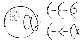 Figure 1
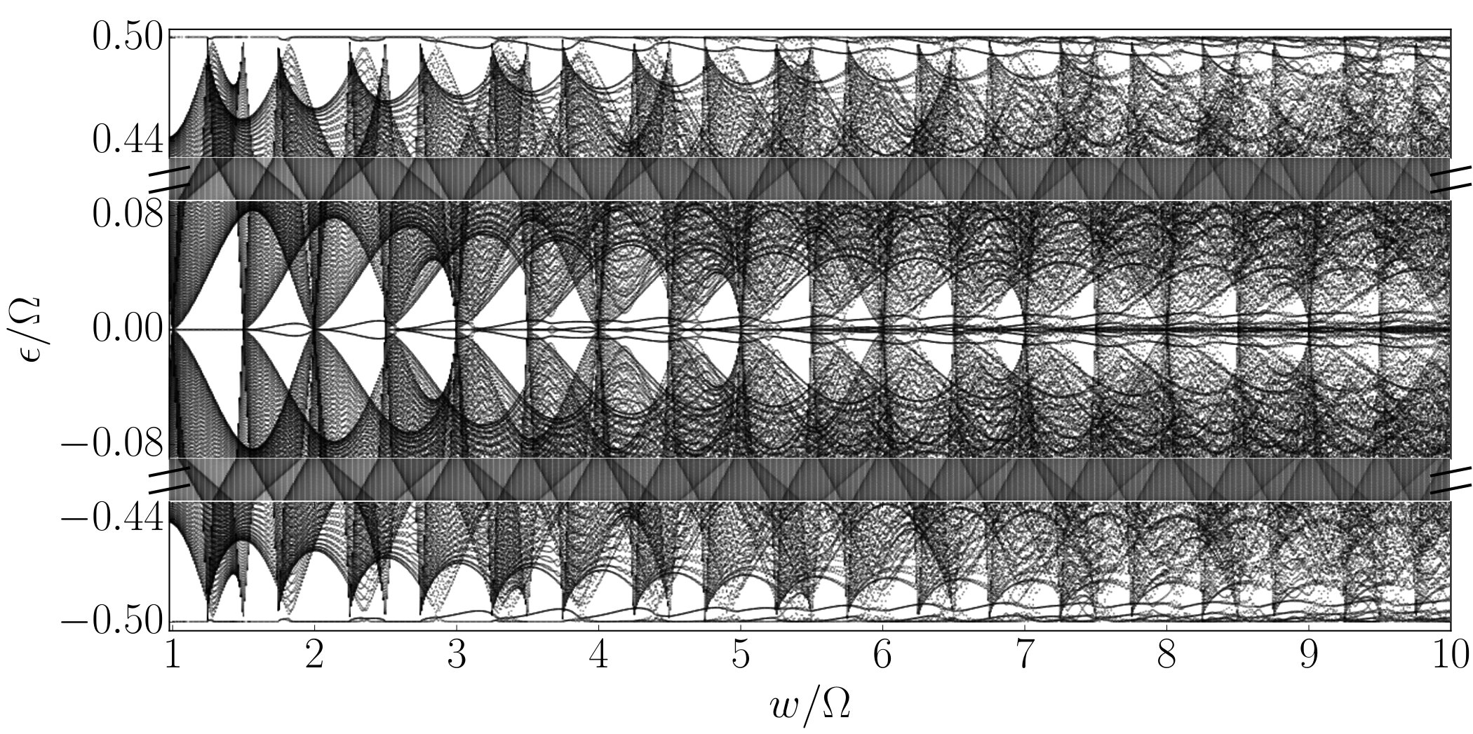 Figure 1
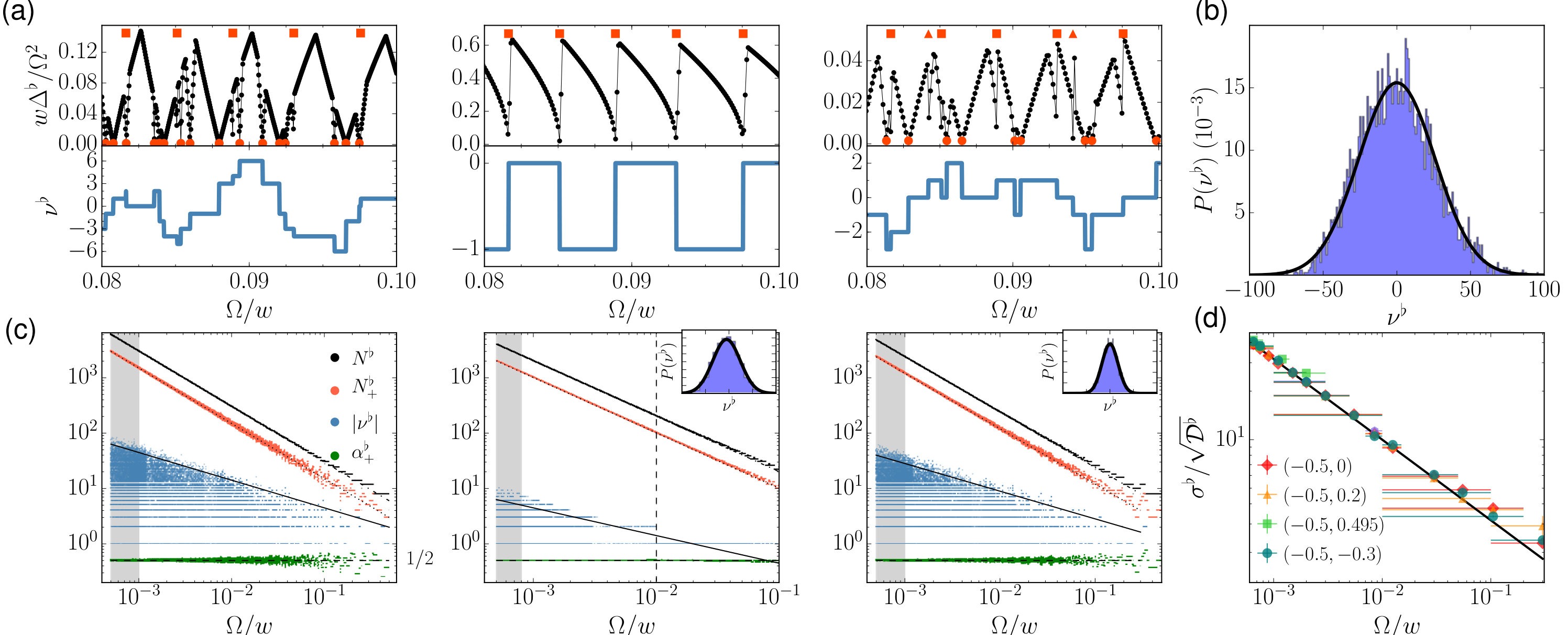 Figure 2
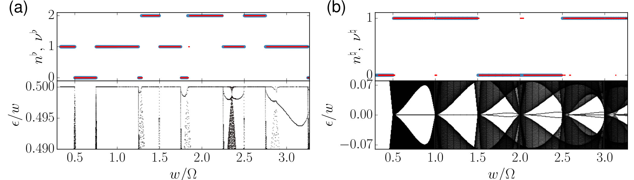 Figure 2
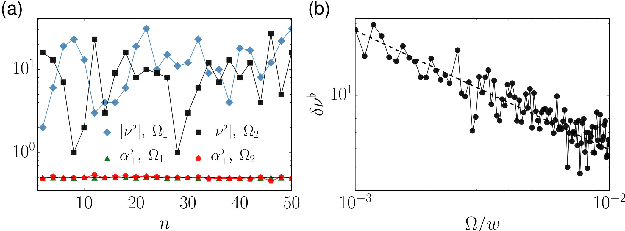 Figure 3
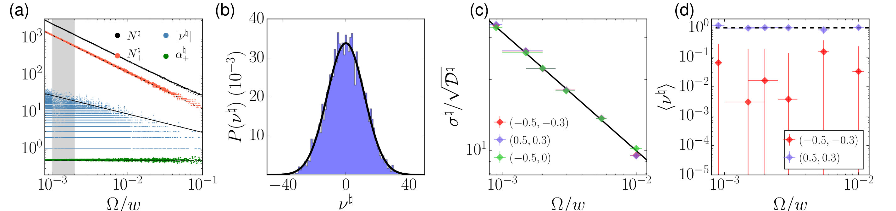 Figure 3
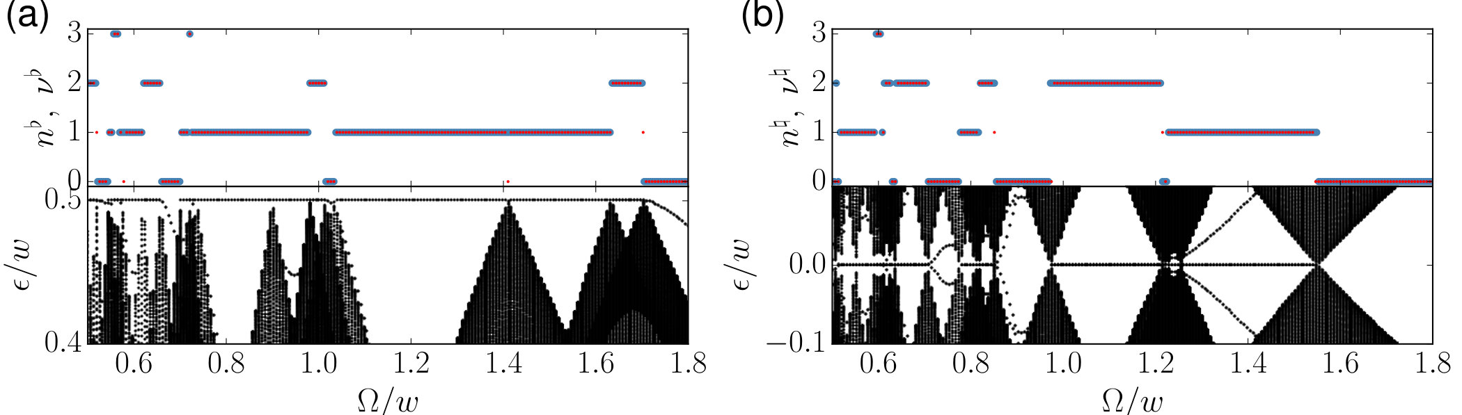 Figure 4
 Figure 4
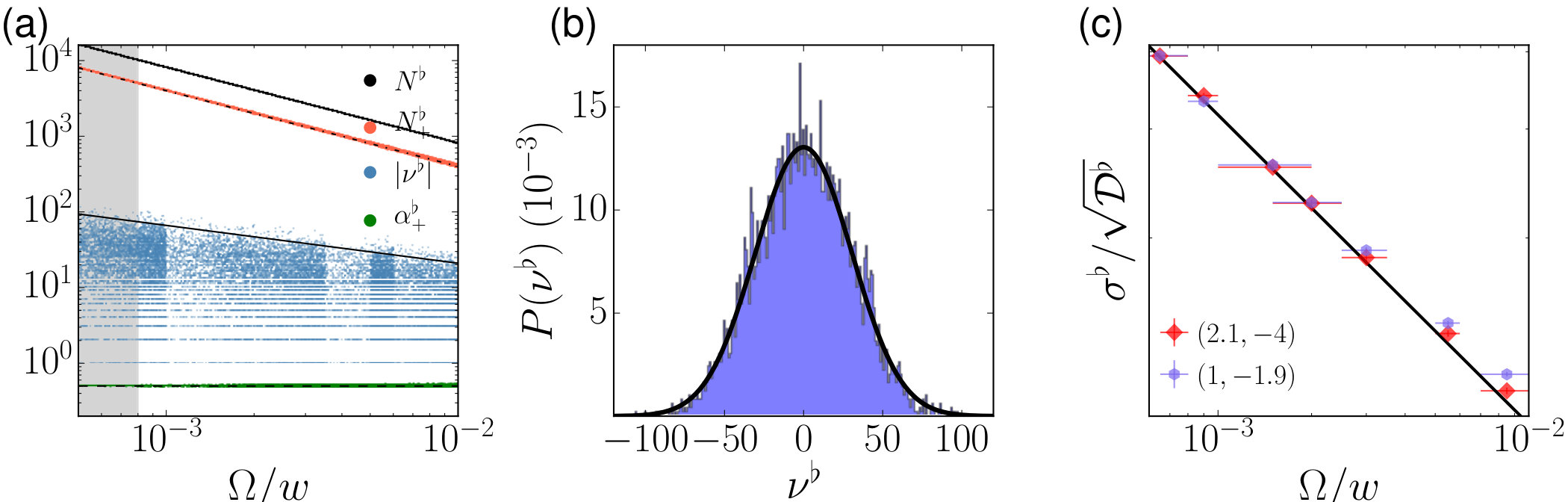 Figure 5
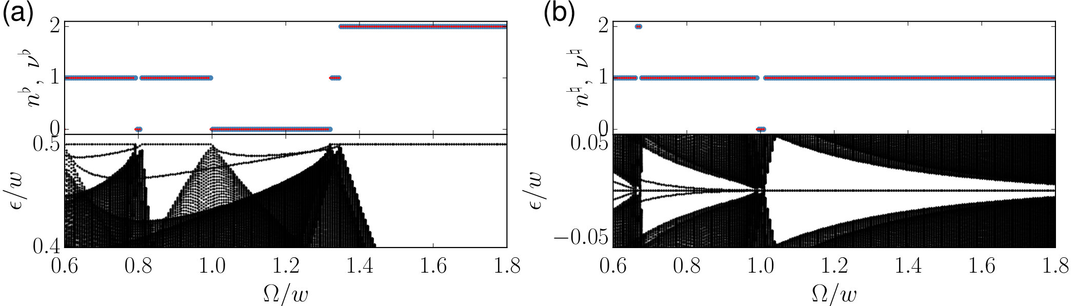 Figure 6
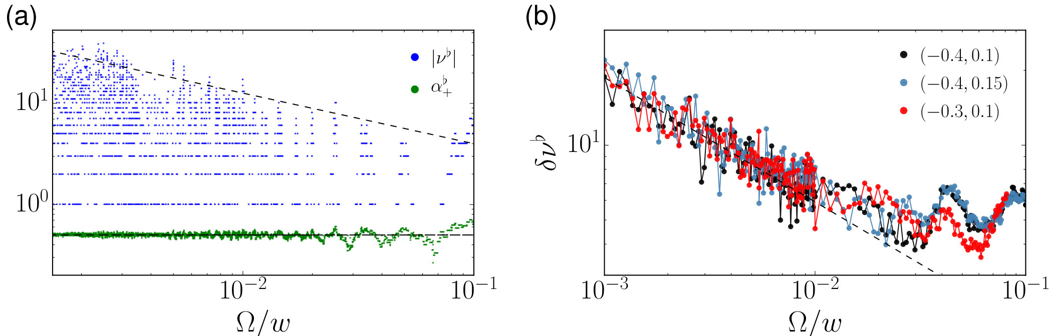 Figure 7
Peer Reviews
No public reviews on file for this paper yet. If you reviewed it on a platform where reviews are public (OpenReview, ICLR, NeurIPS, ICML), you can paste yours below so the community can read it here.
Videos
No videos yet. Explain this paper in a talk, walkthrough, or lecture? Add one.
Universal fluctuations of Floquet topological invariants at low frequencies
M. Rodriguez-Vega
Department of Physics, Indiana University, Bloomington, Indiana 47405, USA
B. Seradjeh
Department of Physics, Indiana University, Bloomington, Indiana 47405, USA
Max Planck Institute for the Physics of Complex Systems, Nöthnitzer Str. 38, 01187 Dresden Germany
Abstract
We study the low-frequency dynamics of periodically driven one-dimensional systems hosting Floquet topological phases. We show, both analytically and numerically, in the low frequency limit , the topological invariants of a chirally-symmetric driven system exhibit universal fluctuations. While the topological invariants in this limit nearly vanish on average over a small range of frequencies, we find that they follow a universal Gaussian distribution with a width that scales as . We explain this scaling based on a diffusive structure of the winding numbers of the Floquet-Bloch evolution operator at low frequency. We also find that the maximum quasienergy gap remains finite and scales as . Thus, we argue that the adiabatic limit of a Floquet topological insulator is highly structured, with universal fluctuations persisting down to very low frequencies.
The behavior of a periodically driven system can be qualitatively different from its equilibrium behavior. Manifestations of such behavior in classical physics include resonances, dynamical stabilization of new steady states, and the period-doubling approach to chaos kapitza1951 ; Fei78a ; ref1d . In quantum systems, the effective Floquet dynamics of a driven systems has been employed as a powerful way to engineer designer Hamiltonians, e.g. by using laser sequences in cold atomic gases. In this way, novel phases of matter have been proposed and realized JotMesDes14a ; AidLohSch15a ; zhang2017x ; choi2017x ; Eck17a .
More recently, it has been understood that a driven system can also exhibit essentially non-equilibrium topological phases, dubbed Floquet topological phases oka2009 ; kitagawa2011 ; lindner2011 ; jiang2011 . Drive parameters, such as the frequency or the shape of the drive (“drive protocol”) have been proposed zhenghao2011 ; dora2012 ; KunSer13a ; KunFerSer14a ; perez2014 ; ref1a ; ref1c ; titum2015 ; KunFerSer16a and used in the lab rechtsman2013 ; WanSteJar13a ; SieLuiLee17a ; ChePanWan18a to engineer a rich array of topological phases not possible in equilibrium systems. The non-equilibrium dynamics at large frequencies is relatively well understood, e.g. within rotating-wave approximation, as a renormalization of the equilibrium parameters of the system blanes2009 ; rahav2003 ; rahav2003b ; bukov2015 ; EckAni15a . The low-frequency regime, on the other hand, remains largely unexplored GomPla13a . This is the relevant regime in solid-state systems driven by ac potentials lindner2011 . It is also important as a way to reduce unwanted heating in the system LazDasMoe14a ; DAlRig14a ; WeiKna17a ; StrEck16a . At a more basic level, it relates to the adiabatic limit as . Numerical studies have reported nonzero Floquet topological invariants as frequency is lowered KunSer13a ; LiuLevBar13a ; TonAnGon13a ; GomDelPla14a ; MikKitYas15a ; ref1b . This raises questions on the nature of adiabatic limit in Floquet topological phases.
In this paper, we study the low-frequency limit of one-dimensional model driven systems that exhibit a rich Floquet topological phase diagram jiang2011 ; KunSer13a . Assuming the driven systems are chirally symmetric Asbóth et al. (2014); ref1b ; dallago2015 , we derive analytical expressions for the Floquet topological invariants and evaluate them numerically over several decades of the drive frequency. We find that these topological invariants not only remain nonzero at low frequencies, but increasingly fluctuate. While at any fixed frequency the invariants are deterministic, over a range of frequencies , the invariants distribute pseudorandomly. We argue that this distribution is universal and in our models is given by a Gaussian, whose width is . We explain this universal behavior by revealing a diffusive process in the evaluation of the invariants and confirm our results numerically.
Specifically, we study one-dimensional driven systems with periodic boundary conditions, with a Hamiltonian of the form , where is the crystal momentum, is a two-component spinor field, and with a model-dependent function. For example, in the Su-Schrieffer-Heeger (SSH) model su1979 ; supp where () is the hopping (modulation) amplitude. In the Kitaev model Kit01a ; supp , after a suitable rotation in the Nambu space, one finds , where is the chemical potential and is the nearest-neighbor pairing amplitude.
These Hamiltonians are particle-hole symmetric, , with eigenvalues . In equilibrium, there are two topologically distinct phases: a topological phase, for in the SSH and for Kitaev model, and a trivial phase otherwise. These two phases are distinguished on the lattice with open boundary conditions by the presence of zero-energy bound states in the topological phase. With periodic boundary conditions, the phases are distinguished by an integer topological invariant or , equal to the winding number
[TABLE]
For a multi-band system, e.g. the SSH-Kitaev WatEzaTan14a ; supp , is matrix-valued and the topological invariant is found by .
When the system is periodically driven, the full dynamics is obtained by solving the Floquet-Schrödinger equation (we are setting ) for the periodic steady states , , with the quasienergy , which we take to be in the Floquet zone . The Bloch evolution operator can then be written as . The full-period evolution operator has eigenstates with eigenvalues . Since the quasienergy is a modular quantity, even a two-band model is characterized by two gaps at Floquet zone center () and Floquet zone edge () Note3 . Thus, for periodic boundary conditions there are two independent topological invariants defined for the quasienergy gaps at Floquet zone center, , and edge, . For open boundary conditions, the corresponding invariants are the number of midgap steady bound states at Floquet zone center and edge supp .
To simplify our discussion, we take the drive protocol to satisfy the chiral reflection symmetry, ; then, the two topological invariants are found Asbóth et al. (2014); supp from the half-period evolution operator U_{k}(\pi/\Omega)\equiv\left(\begin{array}[]{cc}A_{k}&B_{k}\\ C_{k}&D_{k}\end{array}\right), as
[TABLE]
In the static case, is constant and , thus one finds and as expected. For concreteness, we present our results for the SSH model in the following and for other models in the Supplemental Material supp .
At symmetry points , and the half-period evolution operator takes simple forms, and where is the average hopping modulation through one drive cycle. The values , and , can be used to anchor their winding.
To understand the changes in the winding number () we analyze the contour of () in the complex plane as frequency varies (see Fig. 1). At high enough frequency the contour of () is a loop with two crossing points on the real (imaginary) axis at and ( and ); as frequency is lowered the loop twists and untwists, thus changing the number of crossing points on the real (imaginary) axis via two processes: a pair of crossings are “emitted” from () whenever (), where the prime denotes ; on the other hand, a pair of crossings are “absorbed” into () when (). While the rates of these processes depend on the drive protocol, they all scale with ; thus the number of crossings generically grows as . As is lowered, all crossings move back and forth within the unit disk along the real (imaginary) axis at a speed that scales with . When a crossing point of () passes through the origin, the winding () changes. The inversion symmetry of the SSH model ensures that except and ( and ), all other crossings are doubled.
Denoting the momenta at crossing points with , where , the total number of crossings is , where and . The winding numbers, on the other hand, are given by . At any given frequency, , the values of may be computed deterministically from the number of crossings emitted, absorbed, and moved on the corresponding real or imaginary axis. However, as , these numbers grow in an increasingly complex way; thus, over a frequency interval the distribution of crossing points appears random. We posit that this distribution can be modeled by a universal stochastic process of emission, absorption, and motion of crossing points of () Note0 . In the low-frequency limit, our numerics show generically that are equally distributed. Taking this to be true, we may think of as the number of steps taken by a one-dimensional random walker in opposite directions, with the distance from the starting point. Thus, winding numbers are diffusive variables with a protocol-dependent diffusion constant . Here, stands for the average in the stochastic model or, equivalently, the average over the interval . The winding numbers acquire a Gaussian distribution with a width . This is our main result.
Changes in the winding number are concomitant with quasienergy gap closings. This is easy to see at symmetry points , where, for our chirally symmetric protocols, the full-period evolution operator is the square of the half-period evolution operator. At these points, () change by one when and ( and ) vanish, respectively, at and ( and ) for integer . Noting that quasienergies at symmetry points are given by and , it is easy to see they are equal to () exactly at frequencies where () changes. Of course, changes in () are also caused at any frequency () and non-symmetry momenta [], where () vanishes and the gap at () closes. Due to inversion symmetry, the winding numbers at these gap closings change by two. We note that the frequencies and depend on the drive protocol.
To proceed quantitatively, we choose a periodic two-step drive protocol in the SSH model given by for and for . Here, is the dimensionless fraction of the period for the first step of the drive. This family of protocols simplifies the numerical calculations, and allows us to obtain both analytically exact and numerically reliable results over a wide range of frequencies. Note that the modulation is chiral symmetric. This is explicit if we take the origin of time to be at . Calculating the full-period evolution operator, the quasienergies are given by
[TABLE]
where the average and difference bands , with index , indicating . Here, is the angle between the complex variables and . Without loss of generality, we assume . Gap closings at for are obtained when , where and . This is a resonant condition leading to an implicit equation for , which we solve numerically. Furthermore, for , there exist where ; at these points, the gap at closes for .
The winding numbers are found from
[TABLE]
and ,
[TABLE]
Since or and , () and () are real. We note , i.e. .
Focusing on for concreteness and using the explicit forms of , we find that the crossing points that contribute to either or are emitted when or is an integer, and they are absorbed when or is an integer. For and for small enough frequency, we may assume the motion of crossing points yields a nearly uniform distribution along the real axis. Since the winding number varies by 2 only when the crossing two points are on different halves of the real axis, the diffusion constant may be obtained by . In the following, we assume for simplicity.
Our analytical expressions for the two-step drive allow for the exact determination of gap closings; however, in general, quasienergy gaps and topological invariants can only be obtained by numerical solutions. In the special case of a symmetric drive, and , we can calculate the topological invariants exactly: , and when is even and 0 otherwise.
For the numerical solutions, we consider three distinct protocols: the asymmetric protocol, , which is a periodic switch between the equilibrium trivial and the topological phases with the asymmetry parameter ; the critical protocol, , i.e. a periodic switch between the equilibrium trivial and the critical point of the system; and finally, the trivial protocol, , such that the systems is in the equilibrium trivial phase at all times. Our numerical results for are summarized in Fig. 2; our results for are similar supp .
The quasienergy gaps exhibit self-similar patterns, with peaks that scale as . We have benchmarked our numerical calculation with the exact analytical expressions for gap closings, shown on the same plot; the agreement is extremely good. The scaling can be understood within adiabatic perturbation theory RigOrtPon08a ; RodLenSer18a , where the frequency is used as a perturbation parameter. The first-order correction to the quasienergy is the Berry phase of the steady states, which vanishes for our chirally symmetric protocols RodLenSer18a ; MarMoi15a .
The winding number fluctuates as frequency is lowered with an increasing relative amplitude. For an asymmetric protocol, as in Fig. 2(c) center panel, when , we observe the regular step-wise behavior as in the symmetric protocol. However, when , the same fluctuating pattern sets in. We have carried out a detailed analysis of over a wide range of low frequencies. For each frequency , we show , , , and . Both , and scale linearly with , confirming our general arguments. The ratio approaches as the frequency decreases, indicating the diffusive behavior familiar from a random-walk process. Moreover, the range of scales as . For a range of frequencies much lower than other energy scales in the system, we have determine the probability of finding in our numerical histogram. As shown, follows a Gaussian distribution with a width that is given by over several decades of frequency, confirming our general result.
To test our general arguments for the universality of the fluctuations, we have studied other drive protocols and other models, including a model with multiple bands. These numerical studies support our results in all cases. Details are found in the Supplemental Material supp ; here, we present our results for a multi-step protocol in the SSH model approximating . The analytical calculations become increasingly difficult as the number of steps in the drive increases; however, we can still calculate the topological invariants numerically. A typical sampling of our results are shown in Fig. 7. While fluctuates both in magnitude and sign as is varied, the ratio , again indicating a diffusive process. Collecting good statistics over a wide frequency range quickly becomes too expensive. However, since the fluctuations in the winding number result from the twisting and untwisting of the contour , we expect that varying the number of steps should have a similar effect. Indeed, as shown in Fig. 7(b), after averaging over , the root-mean-square .
In conclusion, we have found universal fluctuations in the topological invariants characterizing a Floquet topological phase. We explained these fluctuations by positing a pseudorandom distribution of crossing points of the complex function whose winding number gives the topological invariant. This distribution follows from the diffusive process of emission, absorption, and motion of crossing points as frequency is lowered. Our results show that the limit has a rich structure that is distinct from the simple adiabatic limit: while the topological invariant vanishes Note2 on average, consistent with the adiabatic limit, its fluctuations diverge. These fluctuation may be observed in the noise spectra of relevant quantities such as voltage noise RodFerSer18a , or by spectroscopic measures of the number of Floquet edge modes as recently observed in a photonic crystal emulator ChePanWan18a .
Universal fluctuations in Chern numbers have been studied in quantized classically-chaotic and random matrix theories LebKurFei90a ; WalWil95a . By contrast, we study periodically driven systems, where topology is characterized not just by Chern numbers of a static Hamiltonian, but by independent winding numbers through a drive cycle. In this context, it would be interesting to study if driven systems with different symmetries (say, other than chiral symmetry) can support other universality classes of fluctuations of Floquet topological invariants.
Acknowledgements.
This work was supported in part by BSF grant No. 2014345, NSF CAREER grant DMR-1350663, and the College of Arts and Sciences at Indiana University. M.R.V. acknowledges the support and hospitality of Max Planck Institute for the Physics of Complex Systems.
I Supplemental Material
In this Supplemental Material, we recap, for completeness, the derivation of the Floquet topological invariants in one-dimensional driven systems with a chiral reflection symmetry, and present the details of our numerical studies for driven Su-Schrieffer-Heeger (SSH), Kitaev, and SSH-Kitaev models, as well as the multi-step drive protocol in driven SSH model.
I.1 Topological invariant for driven one-dimensional chiral-symmetric systems
In this section, we briefly outline the derivation of the topological invariant for one-dimensional chiral symmetric systems, following Ref. Asbóth et al. (2014). A driven system has chiral symmetry if there exist a unitary, hermitian, local operator , such that
[TABLE]
where the time-ordered exponential is the full-period evolution operator with the initial time and period for the Hamiltonian . A topological invariant characterizing a chiral-symmetric one-dimensional system with perioidic boundary conditions can be written in the diagonal basis of , where
[TABLE]
as
[TABLE]
where is the lattice momentum.
Now, we say the drive protocol in has chiral reflection symmetry if for some and , one has , where . That is, the drive protocol starting at has a reflection symmetry about . Then, and both satisfy satisfy Eq. (6).
Thus, we can define two topological invariants and . Physically, they can be interpreted as a bulk “sublattice” polarization at times , and . Given that states with quasienergy switch sublattice when they evolve from to , neither nor alone are related to the number of edge states in an open system, instead
[TABLE]
where and are the number of edge states with quasienergy , and , respectively. Using algebraic properties of winding numbers in the diagonal basis of , the authors of Ref. Asbóth et al. (2014) showed that and can be derived from the diagonal and off-diagonal blocks of as , .
I.2 Driven SSH model
The tight-binding Hamiltonian for driven the Su-Schrieffer-Heeger (SSH) model is given by the
[TABLE]
where creates a fermion at lattice site , is the unmodulated hopping amplitude and is the hopping modulation, periodic in time with frequency . For periodic boundary conditions, the crystal momentum is a good quantum number; defining the spinor , where indexes the unit cells, we have , with in the Brillouin zone , and Discrete symmetries of this Hamiltonian include inversion , sublattice , and particle-hole symmetry , which place the static SSH model in the BDI class Chiu et al. (2016). The instantaneous eigenvalues are with .
I.2.1 Quasienergy spectrum
In this section, we consider a driven SSH model with open boundary conditions, and calculate the number of edge states present in the system at given frequency. Fig. 4 shows the quasienergies as a function of the inverse frequency in the range . The system has sites and is driven by a two-step protocol switching between and . States with quasienergies , and are localized at the edge of the system.
Top panel of Fig. 5(a) [(b)] shows (), the number of edge mode pairs with quasienergies (), and are compared with the corresponding topological invariant (). We use the same parameters as in Fig. 4. In order to correctly resolve the quasienergies, we consider a systems with sites for the range , for , and for .
Both quantities are in agreement, as expected from the bulk-boundary correspondence. Deviations are observed at frequencies in proximity to gap closings, where a larger system is required to correctly resolve the spectrum. Bottom panel of Fig. 5(a) [(b)] shows a close-up in the quasienergy spectrum around (). Changes in () occur only when the gap around () closes.
I.2.2 Topological invariant
In this section, we discuss the low-frequency limit of , the topological invariant related to the number of edge states with quasienergy . As discussed in the main text, also presents fluctuations in the low-frequency regime, with exceptions in special cases. For example, in the case of a symmetric drive, with and we obtain .
In general, we have to evaluate the invariant numerically. Fig. 6 summarizes our results. The winding number fluctuates as frequency is lowered with a relative amplitude that grows as . Both and scale linearly with . The ratio approaches as the frequency decreases. Moreover, the range of scales as . All of these properties are similar to the low-frequency behavior of . For a range of frequencies much lower than other energy scales in the system, we have determine the probability of finding in our numerical histogram. As shown, follows a Gaussian distribution with a width that is given by over a decade of frequencies. When the drive protocol is entirely in the static topological (trivial) phase, the probability is centered at ().
I.2.3 Multi-step drive protocol
In this section, we consider a multi-step driving protocol as an approximation to the smooth protocol . For a protocol with steps, the half-propagator is given by
[TABLE]
In the limit we recover the smooth protocol. In Fig. 7(a) we plot the invariant and the ratio as a function of the frequency for a protocol with steps. As in the case of a two-step drive, we find that the ration approaches as the frequency decreases, suggesting a diffusive process. Also, presents fluctuations that grow as . For large , it becomes difficult to accurately calculate the invariant, and collecting enough statistics as a function of frequency to determine the scaling in the low-frequency limit becomes more challenging. However, varying changes the structure of complex function , creating new twists. Therefore, we compute for different frequencies as a function of in the range and consider the average over . In Fig. 7(b), we plot the root-mean-square as a function of frequency and find that it also scales as .
I.3 Driven Kitaev Model
In this section we consider the driven Kitaev model, and study the behaviour of the topological invariants in the low-frequency regime. The Hamiltonian is given by Kitaev (2001)
[TABLE]
where and are the nearest-neighbor hopping and pairing amplitudes respectively, and is the chemical potential. Imposing periodic boundary conditions, and introducing the Nambu spinors , the Hamiltonian can be written as , where This has the particle-hole symmetry . Upon the rotation , the Hamiltonian is transformed to
[TABLE]
as shown in the main text. In this representation, the Kitaev model has the discrete symmetries , and . The instantaneous eigenvalues are .
In a system with open boundary conditions we find one pair of Majorana states at zero energy for , and zero for . At the gap closes. The static topological invariant gives for and zero otherwise.
Choosing a suitable driving protocol, the driven Kitaev model also has chiral symmetry, and the topological invariants are given by and , as for the SSH model. In this work, we choose to drive the chemical potential with the two-step protocol for and for , where . We fix . The bottom panels in figure 8 show the quasienergy spectrum for a chain with sites in the frequency range around the Floquet zone edge and center. Top panel (a) [(b)] shows the topological invariant () underneath the number of states with quasienergy (), shown in red. These quantities are in agreement. Differences can be found at frequencies where the corresponding quasienergy gap is closed.
We now evaluate the topological invariants numerically in the low-frequency regime. For concreteness, we focus on . Our results are summarized in Fig. 9. As for the SSH model, we find that the range of scales as , both and scale linearly with , and the ratio approaches as the frequency decreases. Furthermore, the probability follows a Gaussian distribution with width .
I.4 Four-band driven Kitaev-SSH Model
In this section we consider the Kitaev-SSH model Wakatsuki et al. (2014). The Hamiltonian is given by
[TABLE]
where labels the unit cells, and , label the sublattices in each unit cell, () and are the intra-cell (inter-cell) hopping and pairing amplitudes respectively and is the chemical potential. If we consider periodic boundary conditions, and define the spinor , the momentum-dependent Hamiltonian takes the form Wakatsuki et al. (2014)
[TABLE]
where , and . For our purpose, the most important feature of this model is that it has four energy bands, given by
For we have two pairs of zero-energy states localized at the edge, while for we have only one pair. For there are no zero-energy states. For simplicity, now on we consider the case , although is possible to also consider finite chemical potentials. The chiral basis for this model is defined by the transformation where and for are the Pauli matrices in particle-hole and sublattice space, and .
We choose the driving protocol for and for , where to ensure that the driven system posses chiral symmetry. As before, we will fix . In Fig. 10, the bottom panels show the quasienergy spectrum for a driven chain with sites around the Floquet zone edge (a) and center (b). The rest of the parameters used are , , and . Top panel (a) [(b)] shows the topological invariant () underneath of (), the number of states with quasienergy (), shown in red. These quantities are in agreement, as expected from the bulk-edge correspondence.
The topological invariants are derived from the half-period evolution propagator U_{k}(\pi/\Omega)\equiv\left(\begin{array}[]{cc}A_{k}&B_{k}\\ C_{k}&D_{k}\end{array}\right), where and are now matrices. The winding numbers are given by , and where As explained in the main text, for multi-band systems, the invariant is still defined by the winding of a complex functions, and . The evaluation of is done numerically, and our results are summarized in Fig. 11. As in the other two driven chiral-symmetric systems, the SSH model and the Kitaev model, we find that fluctuates as frequency is lowered. The probability also follows a Gaussian distribution, with a width given by .
References
- Asbóth et al. (2014)
J. K. Asbóth, B. Tarasinski, and P. Delplace, Phys. Rev. B 90, 125143 (2014).
- Chiu et al. (2016)
C.-K. Chiu, J. C. Y. Teo, A. P. Schnyder, and S. Ryu, Rev. Mod. Phys. 88 (2016).
- Kitaev (2001)
A. Y. Kitaev, Physics-Uspekhi 44, 131 (2001).
- Wakatsuki et al. (2014)
R. Wakatsuki, M. Ezawa, Y. Tanaka, and N. Nagaosa, Phys. Rev. B 90, 014505 (2014).
The reference list from the paper itself. Each links out to its DOI / PubMed record.
- 1(1)
- 2(2) P. Kapitza, Soviet Phys. JETP 21 , 588 (1951).
- 3(3) M. J. Feigenbaum, J. Stat. Phys. 19 , 25 (1978).
- 4(4) J. Wang and J. Gong Phys. Rev. A 77 , 031405(R) (2008).
- 5(5) G. Jotzu, M. Messer, R. Desbuquois, M. Lebrat, T. Uehlinger, D. Greif, and T. Esslinger, Nature 515 , 237 (2014).
- 6(6) M. Aidelsburger, M. Lohse, C. Schweizer, M. Atala, J. T. Barreiro, S. Nascimbene, N. R. Cooper, I. Bloch, and N. Goldman, Nat. Phys. 11 , 162 (2015).
- 7(7) J. Zhang, P. W. Hess, A. Kyprianidis, P. Becker, A. Lee, J. Smith, G. Pagano, I.-D. Potirniche, A. C. Potter, A. Vishwanath, N. Y. Yao, and C. Monroe, Nature 543 , 217 (2017).
- 8(8) S. Choi, J. Choi, R. Landig, G. Kucsko, H. Zhou, J. Isoya, F. Jelezko, S. Onoda, H. Sumiya, V. Khemani, C. v. Keyserlingk, N. Y. Yao, E. Demler, and M. D. Lukin Nature 543 , 221 (2017).