Public transportation in UK viewed as a complex network
R. de Regt, C. von Ferber, Yu. Holovatch, M. Lebovka

TL;DR
This study analyzes UK public transport networks using complex network theory, revealing stability characteristics and fractal properties that can inform improvements in efficiency and resilience.
Contribution
First to assess the stability of UK national public transport networks using complex network methods and fractal analysis.
Findings
Identified stability differences among UK PTNs
Revealed fractal properties related to station service areas
Proposed key performance indicators based on network features
Abstract
In this paper we investigate the topological and spatial features of public transport networks (PTN) within the UK. Networks investigated include London, Manchester, West Midlands, Bristol, national rail and coach networks during 2011. Using methods in complex network theory and statistical physics we are able to discriminate PTNs with respect to their stability; which is the first of this kind for national networks. Moreover, taking advantage of various fractal properties we gain useful insights into the serviceable area of stations. These features can be employed as key performance indicators in aid of further developing efficient and stable PTNs.
Click any figure to enlarge with its caption.
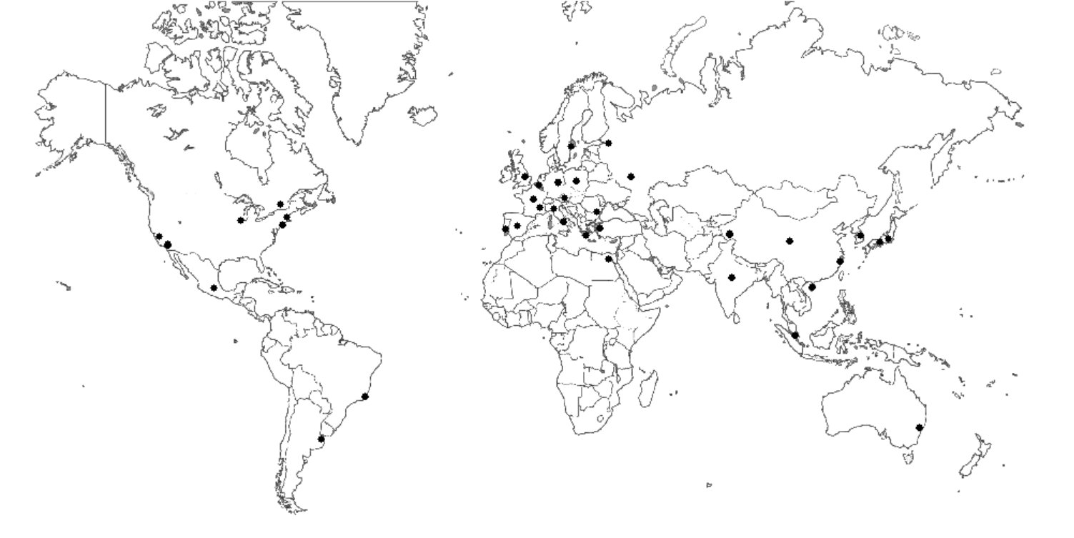 Figure 1
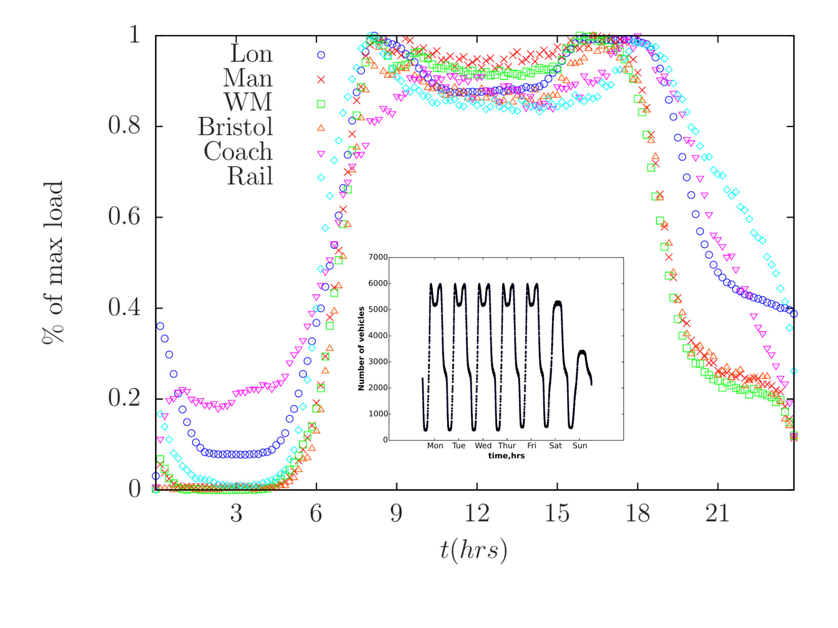 Figure 10
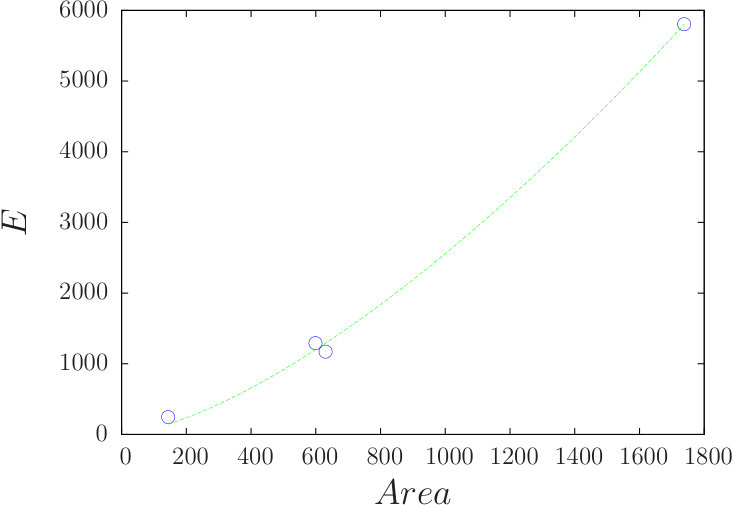 Figure 11
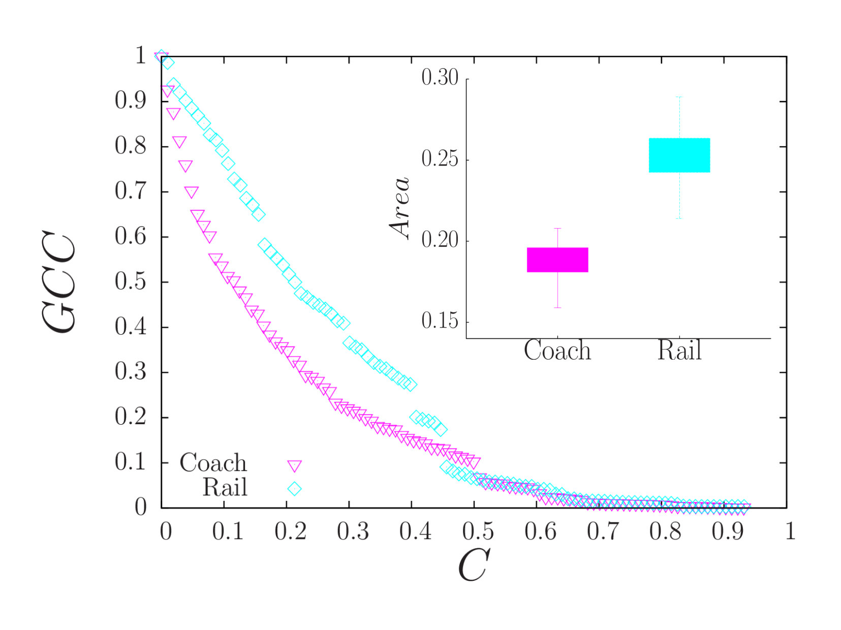 Figure 8
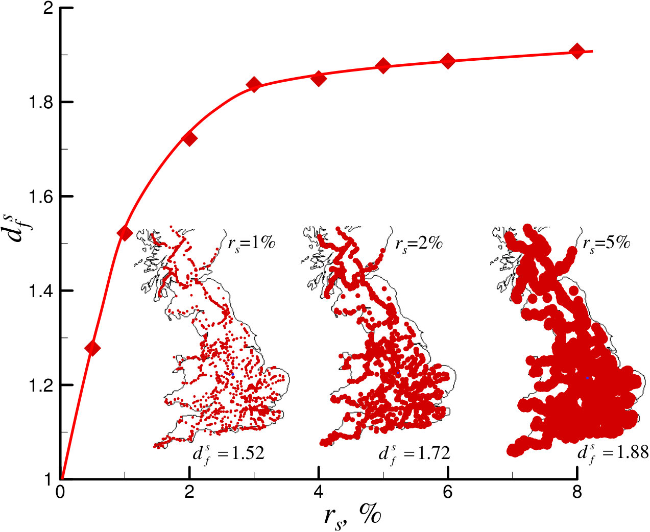 Figure 9
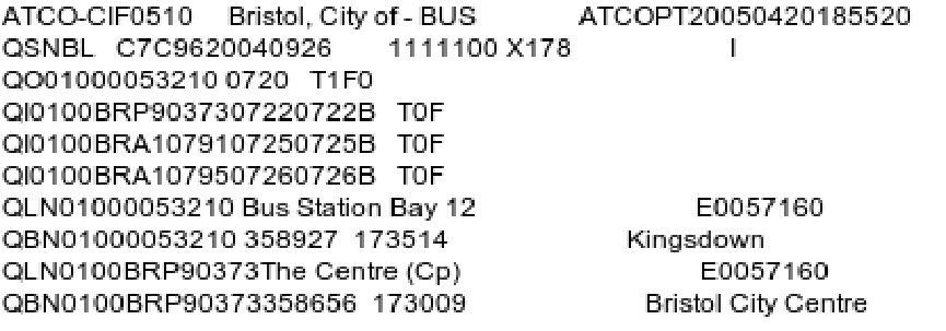 Figure 2
 Figure 3
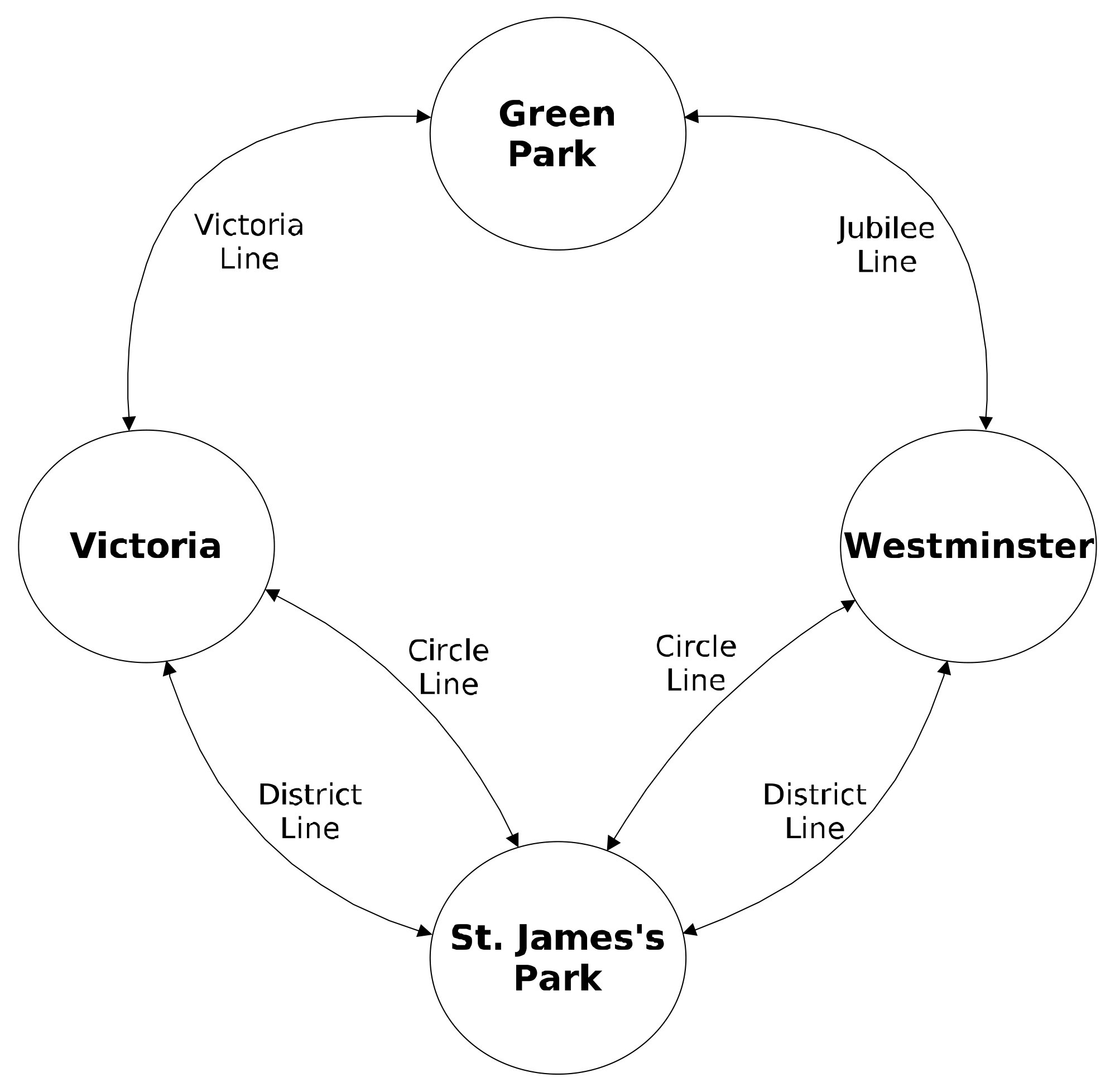 Figure 3
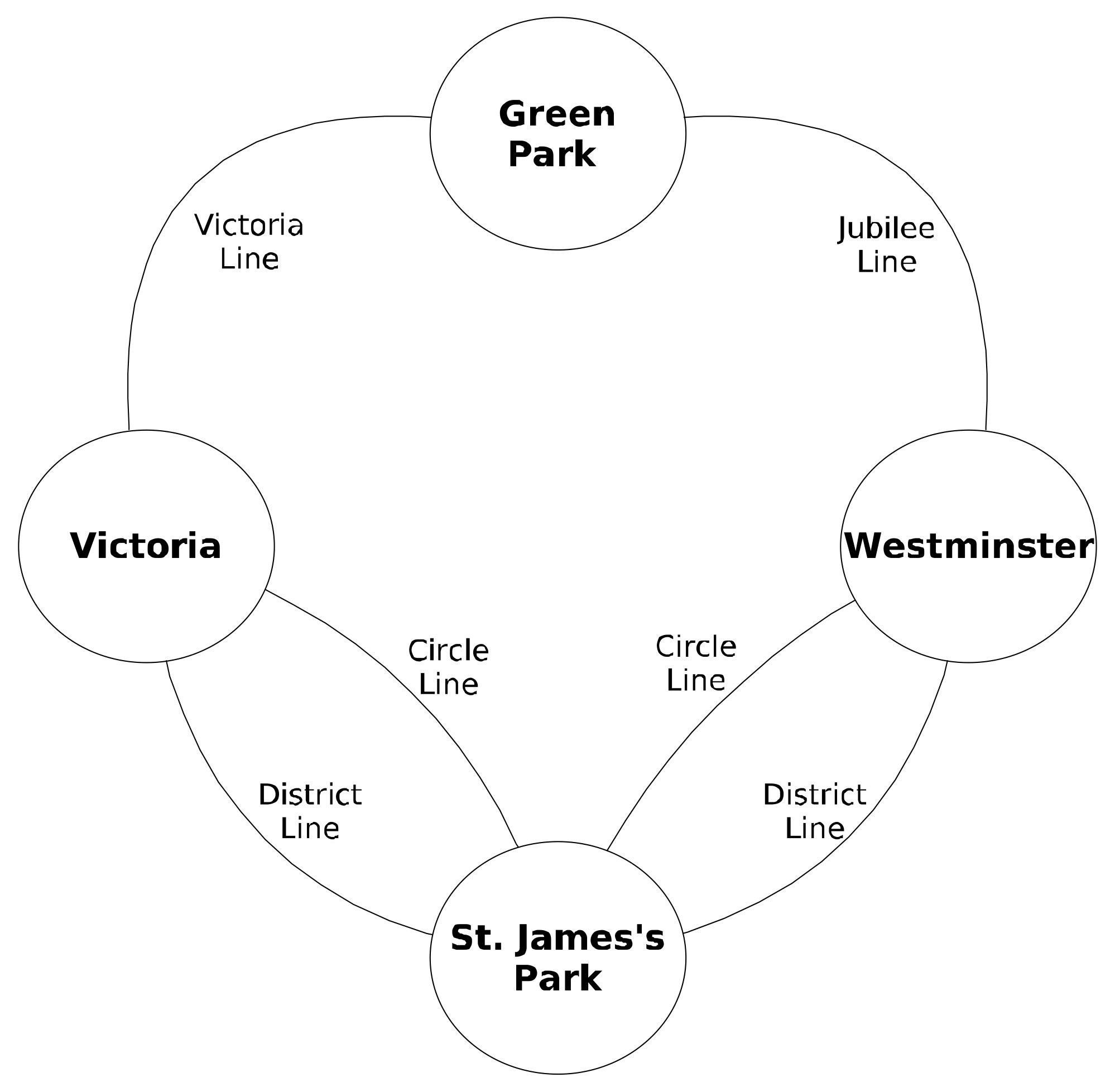 Figure 3
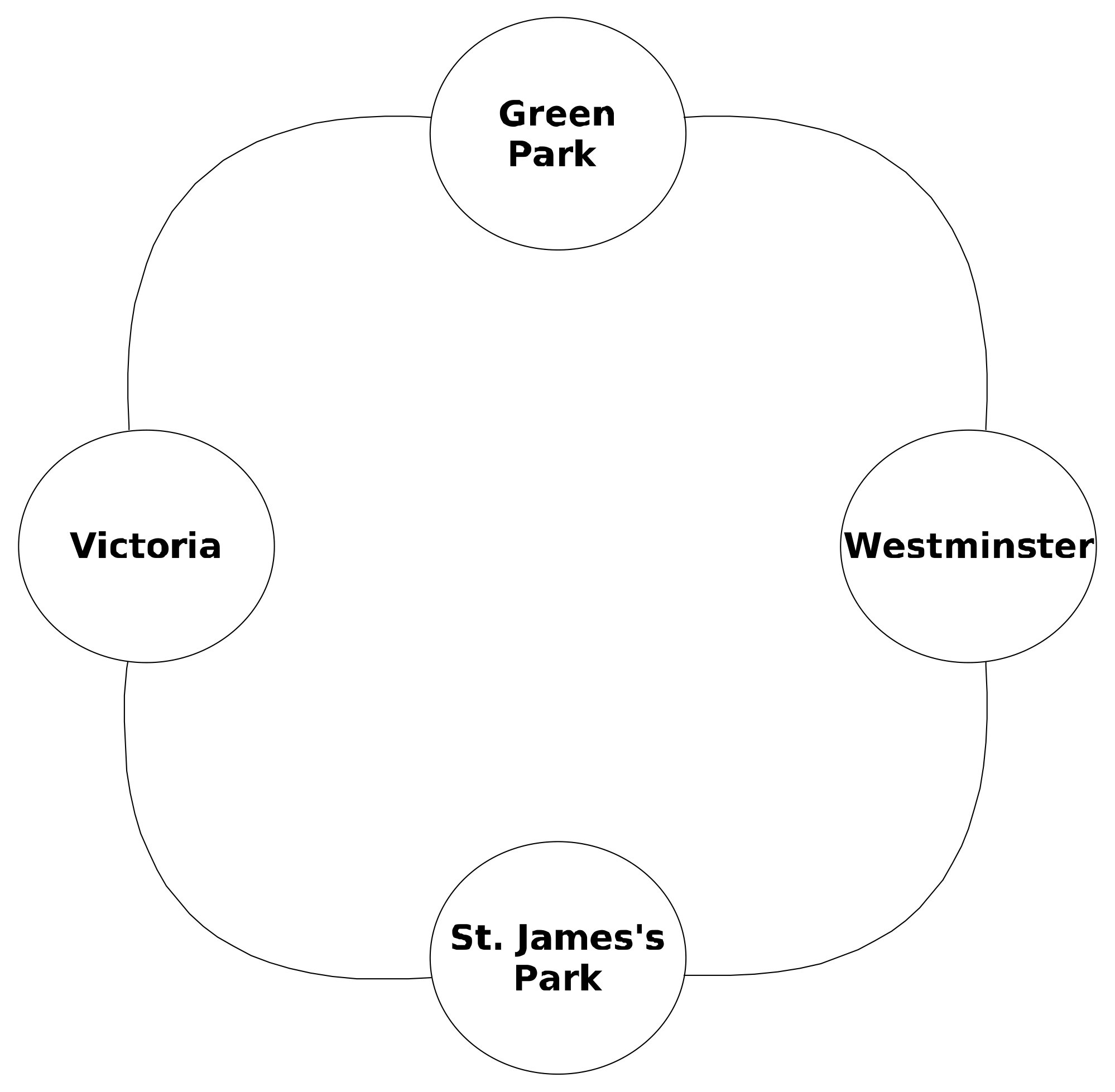 Figure 3
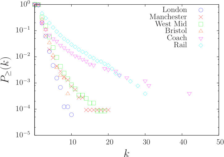 Figure 4
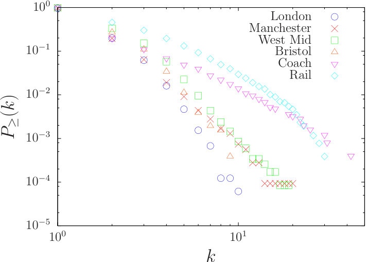 Figure 4
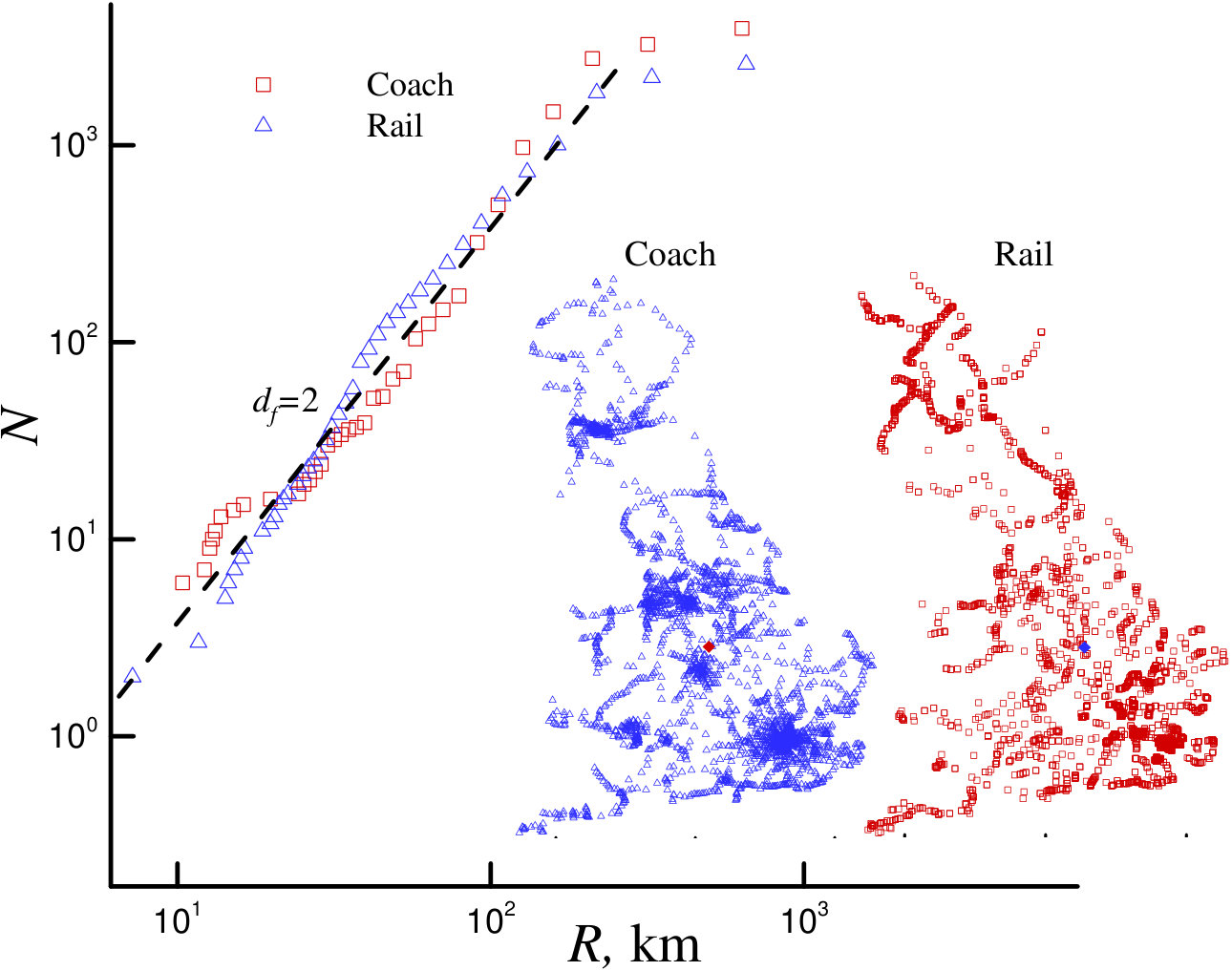 Figure 5
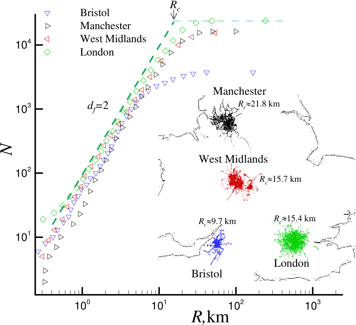 Figure 6
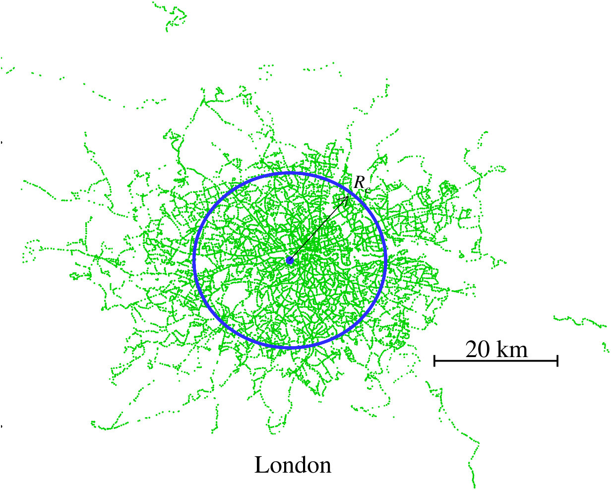 Figure 7
| Networks | GCC | ||||||||||||||
|---|---|---|---|---|---|---|---|---|---|---|---|---|---|---|---|
| Coach | 2.58 | 12.17 | |||||||||||||
| Rail | 3.46 | 20.03 | |||||||||||||
| Bristol | 2.40 | 6.58 | |||||||||||||
| Manchester | 2.29 | 5.87 | |||||||||||||
| West Mid | 2.56 | 7.75 | |||||||||||||
| London | 2.26 | 5.56 |
| City | Type | |||||
|---|---|---|---|---|---|---|
| Dallas | B | 5366 | 117 | 2.35 | 5.49 | 45.86 |
| London | B | 16397 | 767 | 2.46 | 4.25 | 21.38 |
| West Midlands | B | 11743 | 521 | 2.56 | 3.10 | 22.54 |
| Manchester | B | 10742 | 862 | 2.56 | 4.36 | 12.46 |
| Istanbul | BST | 4043 | 414 | 2.69 | 4.04 | 9.72 |
| Los Angeles | B | 44629 | 1881 | 2.73 | 4.85 | 23.73 |
| Bristol | B | 2580 | 172 | 2.74 | 3.56 | 15.00 |
| Berlin | BSTU | 2992 | 211 | 3.16 | (4.30) | 14.18 |
| Düsseldorf | BST | 1494 | 124 | 3.16 | 3.76 | 12.00 |
| Hamburg | BFSTU | 8084 | 708 | 3.26 | (4.74) | 11.33 |
| Rome | BT | 3961 | 681 | 3.67 | (3.95) | 5.87 |
| Taipei | B | 5311 | 389 | 4.02 | (3.74) | 13.6 |
| Sydney | B | 1978 | 596 | 4.37 | (4.03) | 3.31 |
| Hong Kong | B | 2024 | 321 | 5.34 | (2.99) | 6.31 |
| Saõ Paolo | B | 7215 | 997 | 5.95 | 2.72 | 7.23 |
| Paris | BS | 3728 | 251 | 6.93 | 2.62 | 14.84 |
| Moscow | BEST | 3569 | 679 | 7.91 | (3.22) | 5.23 |
| Coach | Rail | Bristol | Manchester | West Mid | London | |
|---|---|---|---|---|---|---|
Peer Reviews
No public reviews on file for this paper yet. If you reviewed it on a platform where reviews are public (OpenReview, ICLR, NeurIPS, ICML), you can paste yours below so the community can read it here.
Videos
No videos yet. Explain this paper in a talk, walkthrough, or lecture? Add one.
Public transportation in Great Britain viewed as a complex network
\nameRobin de Regta,c, Christian von Ferbera,c, Yurij Holovatchb,a,c and Mykola Lebovkad,e CONTACT Robin de Regt. Email: [email protected] aApplied Mathematics Research Centre, Coventry University, Coventry, CV1 5FB, UK; bInstitute for Condensed Matter Physics, National Acad. Sci. of Ukraine,UA-79011 Lviv, Ukraine; c Collaboration & Doctoral College for the Statistical Physics of Complex Systems, Leipzig-Lorraine-Lviv-Coventry; dF.D. Ovcharenko Institute of Biocolloidal Chemistry, National Acad. Sci. of Ukraine, 03142 Kyiv, Ukraine;e Sorbonne Universités, Université de Technologie de Compiègne, EA 4297, Centre de Recherches de Royallieu, BP 20529-60205 Compiègne Cedex, France
Abstract
In this paper we investigate the topological and spatial features of public transport networks (PTN) within Great Britain. Networks investigated include London, Manchester, West Midlands, Bristol, national rail and coach networks during . Using methods in complex network theory and statistical physics we are able to discriminate PTN with respect to their stability; which is the first of this kind for national networks. Taking advantage of various fractal properties we gain useful insights into the serviceable area of stations. Moreover, we investigate universal load dynamics of these systems. These features can be employed as key performance indicators in aid of further developing efficient and stable PTN.
keywords:
public transit; complex networks; fractals
1 Introduction
Over the last few decades society has become increasingly dependent on public transport to facilitate commuters and the movement of commodities on both local and global scales. With transport having such a significant role in the economy of cities and countries it is becoming increasingly important to develop cost effective methods to evaluate the efficiency and robustness of existing public transport networks.
One approach to study these networks is offered through complex network science, a recently established research field with a firm theoretical background and a broad range of applications. It has successfully explained numerous phenomena that have emerged in natural and man made systems involving separate agents connected via various types of interactions (Albert and Barabási, 2002; Dorogovtsev and Mendes, 2003; Barrat et al., 2008; Newman, 2010).
Very often underlying networks do not have direct geometrical interpretations (Guimera, 2007), for example in social networks that involve collaboration, acquaintances and friends. Here, one quantifies the network in terms of its topological features: node degree distribution, connectivity, clustering, as will be discussed in more detail below and further elaborated on in the appendix.
There are however networks which are shaped by their embedding in geometric space (Barthélemy, 2011), like transport networks for example. In addition to their topological properties, these networks are naturally quantified in terms of their geometric features. The latter being primarily defined by spatial coordinates of nodes and include Euclidean distances between nodes.
The purpose of this paper is to investigate the properties of PTN in Great Britain (GB) using both complex networks (i.e. topological) as well as spatial descriptions in order to gain useful insights into robustness and efficiency of PTN. Currently, there exists a relatively broad literature on the application of a complex networks for public transport analysis (see, in particular, the discussion below). Here, we add to the existing analysis and further explore certain topological measures which can be used to classify PTN with respect to their stability to random failures. We add to this analysis by studying the fractals properties of these systems which offer insight into the serviceability and efficiency of PTN. Together both the topological and spatial features studied here may contribute to a better understanding of the underlying mechanisms governing PTN growth and modeling. This ignores important concepts of transportation, passenger flow and service frequency being beneath the major ones. In an attempt to avoid such types of flaws, we complete our study by analysing some features of PTN dynamics and network load.
Another objective of our paper is to attract the interest of academics and practitioners dealing with public transportation networks in furthering the applications of the methods discussed here. So far, application of these methods to transportation networks has been extensively discussed and thoroughly approved on the pages of specialised physical and complex system journals see e.g. the list of references at the beginning of the next section. Addressing this paper to the journal devoted to transportation we pursue an aim to interest its readers in more intensive practical application of the matters discussed here.
The paper is organised as follows. In section 2 we present a brief review of the literature devoted to PTN topological and spatial analysis. Section 3 describes the database we use. The main results of our analysis are presented in section 4, where we discuss topological and spatial aspects of several PTN: those of Greater London, Greater Manchester, West Midlands, Bristol, and the national rail and coach networks of GB. Conclusions and an outlook are given in section 5.
2 Review
Topology
Although the application of complex network analysis to the study of PTN has started comparatively recently, sufficient information has been accumulated to extract some general conclusions. Since 2002 when Latora and Marchiori first published their work analysing the topological properties of the Boston subway (Latora and Marchiori, 2002) many other similar studies have been performed all over the world. This can be seen in Fig 1 where black dots indicate approximately where the topological features of PTN have been analysed. These PTN have ranged in size from to stations. The types of PTN that have been investigated include the subway (Latora and Marchiori, 2002; Seaton and Hackett, 2004), bus (Xu et al., 2007a; Sui et al., 2012; Yang et al., 2011; Guo et al., 2013), rail (Sen et al., 2003), air (Sun et al., 2016, Pien et al., 2015; Guida and Maria, 2007; Guimera et al., 2005; Zang et al., 2010), maritime (Xu et al., 2007b; Hu and Zhu, 2009; Lui et al., 2017) and various combinations of these (von Ferber et al. 2009; Sienkiewicz and Hołyst, 2005; Soh et al., 2010; Zhang et al., 2013, 2014; Alessandretti et al., 2015; Zhang et al. 2016a, 2016b.
Currently, in complex network science a number of topological representations of PTN are in use for the purpose of extracting various types of information. Different representations may be implemented by attributing different constituents of the real world network to graph nodes and edges. For example, one can represent each PTN station as a graph node and join all nodes that form part of a particular route to make a complete subgraph. Different subgraphs will be joined together due to common stations that are shared by different routes. Such a representation has been called -space (Sen et al., 2003; Seaton and Hackett, 2004; Sienkiewicz and Hołyst, 2005; von Ferber et al., 2009; Xu et al., 2007; Ghosh et al., 2010). It is useful in particular for determining the mean number of vehicle changes one has to take when traveling between any two points on the network. In the so-called -space (von Ferber et al., 2007; Chang et al., 2007) one constructs a bipartite graph that contains nodes of two types: node-stations and node-routes. Only nodes of different types can be linked: a node-station is linked to the node-route if it belongs to that route. One can pass from such representation to a graph where only nodes of one type are present. This is achieved by a single mode projection, when all nodes of a similar type which are linked to a common node of another type are represented as a complete subgraph. Naturally, the single mode projection of the -space graph to the nodes-stations leads to -space. In turn, an analogous projection to the nodes-routes leads to the so-called -space (von Ferber et al., 2009). Here, one considers how routes are connected to each other. In -space if any two routes service the same station they are obviously linked. In Fig 2 we show a schematic view of the situation in the -space (as this is the topology we use in this study).
As it can be seen from Fig 2, the -space representation is constructed following a simple process. If two stations are adjacent in a route a link is formed between the two stations. However, if there are multiple routes going through the same two stations, -space will not reflect this as it will not permit multiple links. This topology is ideal for studying the connectivity of networks for example calculating metrics like mean path length , Giant Connected Component (GCC) and other similar metrics, see the Appendix for definitions, here and below. This space is probably the most commonly used topology and has been applied in many different studies on PTN (Latora and Marchiori, 2001; Sienkiewicz and Hołyst, 2005; von Ferber et al., 2005; Angeloudis and Fisk, 2006; Xu et al., 2007; Ferber et al., 2009). These networks can be analysed as a simple graph with either no weights or as a weighted graph (Latora and Marchiori, 2002). In Latora and Marchiori (2002) it is argued that weighted networks provide more realistic information on PTN especially with regard to . This is because would effectively measure the time or distance taken rather than just the number of stations traveled between two given stations which is where the unweighted network is losing information. It has been argued in Kosmidis et al. (2008) that the spatial embedding (distribution of nodes in Euclidean space) does affect its properties and should be considered when analysing networks that are spatially embedded.
Using networks provides access to different observables quantifying general PTN properties: distributions of node degrees, clustering, assortativity, shortest path length and small-worldedness. As research has progressed other features have become of interest for example how different routes tend to show ’harness’ behavior i.e. follow similar paths for a certain number of stations. This feature was analysed in von Ferber et al. (2005); von Ferber et al. (2009); Berche et al. (2009), where the harness distribution defined as the number of sequences of consecutive stations that are serviced by parallel routes. A similar feature has been treated for weighted networks in Xu et al. (2007). Both methods produce power law distributions for their respective networks.
The criticality of nodes in the international air transportation country networks has been studied in detail (Sun, X., Wandelt, S., & Coa, X., 2017). Different criticality techniques that account for the unweighted structure of air transportation networks, complex network metrics with passenger traffic as weights, and ticket data-level analysis were applied. PTN robustness to targeted and random removal of their constituents (attacks) have also been considered (Sun, X., Wandelt, S., & Zanin, M., 2017, Pien et al., 2015; Berche et al., 2009; Leu et al., 2010; Berche et al., 2012; von Ferber et al., 2012, Bozza et al., 2017, Xing et al., 2017). One of the goals of these studies is to present criteria, that allow for a priori quantification of the stability of real world correlated networks of finite size and to confirm how these criteria correspond to analytic results available for infinite uncorrelated networks. The analysis focused on the effects that defunct or removed PTN constituents (stations or joining links) have on the properties of PTN. Simulating different directed attack strategies, vulnerability criteria have been derived that result in minimal strategies that have significant impact on these systems.
The above empirical research has revealed that PTN constructed in cities with different geographical, cultural and historical background share a number of basic common topological properties: they appear to be strongly correlated structures with high values of clustering coefficients and comparatively low mean shortest path values, their node degree distributions are often found to follow exponential or power law decay (the last case is known as scale free behaviour (Barabási and Albert, 1999)). In turn, collected empirical data has lead to the development of a number of simulated growth models for PTN. In Berche et al. (2009) interacting self avoiding walks on a D lattice with preferential attachment rules are applied to produce similar statistics to real world PTN. In Torres et al. (2011) an optimisation model for line planning is discussed considering the competing interests in maintaining a quality service whilst minimising costs. In Yang et al. (2011) PTN are grown a route for each time step using an ideal -depth clique topology. In Sui et al. (2012) the optimised growth of a route is considered by using two competing factors: investors and clients; clients want the route to be as straight as possible to save time whereas investors want the routes to meander in order to collect as many passengers to maximise profits. As it has been shown recently (Louf et al. (2014)), the cost-benefit analysis accounts for the scaling relations that govern dependency of the PTN characteristics with the socio-economical features of the undelying region.
In most of the papers cited above the main subject of analysis was topology and its impact on the properties of PTN. This type of analysis has lead to substantial progress in understanding the collective phenomena taking place on PTN. For example, the vulnerability of PTN to random failures and targeted attacks appears to be tightly connected to the distribution of nodes of high degree (hubs) (Berche et al., 2009; Berche et al., 2012; von Ferber et al., 2012). Moreover, the analysis of network topology allows for the singling out of the most important nodes that control network integrity and to form alternative methods to construct robust and efficient PTN.
Geospace
Another essential ingredient to be considered in parallel with the analysis of PTN topological properties is the spatial embedding of PTN. There have been far less of these studies when compared to topological studies. This is mainly due to the lack of available data on the spatial coordinates of PTN. The notion of a fractal (non-integer) dimension is often used to quantify the development and growth of cities including their communication and transportation systems. City growth has been shown to exhibit self-similar behaviour, an observation that might imply a universality of processes that drive city agglomeration and clustering (Batty, 1994; Batty, 2008). Moreover, several physical growth processes that are known to lead to such geometry (percolation or diffusion limited aggregation) have been exploited to explain such growth in cities (Batty, 1994; Batty, 2008; Makse et al., 1995; Holovatch et al., 2017).
There have been a few studies that directly consider PTN spatial analysis which mainly focus on modes of transport such as railway and subway (Sun et al., 2017; Sui et al., 2012; Benguigui and Daoud, 1991; Benguigui, 1995; von Ferber and Holovatch, 2013; Guo et al., 2012; von Ferber et al., 2009; Frankhauser, 1990; Thibault, 1987; Kim et al., 2003) and with the availability of data improving more studies are sure to follow. One of the earliest studies is that of Benguigui and Daoud (1991) measuring the fractal dimension of the Paris subway and railway network by counting the number of stations within a radius for a given centre as a function of the radius . In Sui et al. (2012) the end to end mean distance of routes in nine Chinese cities is computed while in von Ferber et al. (2009) is calculated as a function of the number of stations. In von Ferber and Holovatch (2013) the distribution of these inter station distances are analysed and are found to follow Levy flight distributions. In Sun et al. 2017 they consider how the fractality of worldwide airports network effect network metrics such as nodes, edges, density, assortativity, modularity and communities.
These real world transportation networks have been characterised by varying results (Kim et al., 2003; Benguigui and Daoud, 1991; Benguigui, 1992; Frankhauser, 1990; Thibault, 1987; von Ferber and Holovatch, 2013). In particular, in Thibault (1987) three Lyon regions for rail, bus and drainage networks were shown to have fractal dimensions of ranging between , and respectively. These fractal dimensions all show that as the radius from the centre of a city increases the amount of rail, bus and drainage decreases sub-linearly. Rail displays the largest values of fractal dimensionality with the least variance thus indicating that the length of track decreases more slowly than the number of bus stations as the distance is increased from the centre of the city. The Stuttgart railway fractal dimension was found to be (Frankhauser, 1990) and for the Paris railway the value was obtained (Benguigui, 1992). The Rhinetowns and Moscow railways exhibited exponents of and the Paris metro (Benguigui and Daoud, 1991). For the Seoul transportation network the exponents were measured as for stations and for the railway tracks (Kim et al., 2003).
The majority of the above mentioned papers considered either topological or spatial properties. A particular feature of the study we present below is a cumulative analysis of both topological and geographical characteristics. Moreover, to make predictive power of our empirical observations more obvious, we complete our study by analysing some features of PTN dynamics and network load. To this end we have chosen to consider six GB PTN using the data available on the National Transport Data Repository (Data, 2012). Out of those, two PTN operate on an nation-wide scale (national coach and rail networks) and the remaining four are PTN of Bristol, Manchester, West Midlands and Greater London. By this choice we attempted to have examples of areas of different geographical and economical scales. In turn, this enables one to seek for general (universal) characteristics of transportation system as a whole. In the next section we explain the origin of the data and how it will be used in our analysis.
3 Description of PTN database
The data for this study originates from the National Transport Data Repository (NTDR) website (Data, 2012). The website has an Open Government License meaning it is open to the public and it contains information on public transport travel and facilities throughout the GB for the years to and including 111 This data has not been updated so far. The reference Gallotti and Barthélemy (2015) is based on an older version of 2010.. The information provided is a yearly snapshot of the public transport network for a sample week in each year. The week on which the data is usually recorded is either the first or second week in October to avoid recording during school holidays or other seasonal variations which are at a minimum during this period according to NTDR.
The data is collected and assembled following a decentralised system where individual regional travel lines (RTL) are responsible for recording the travel within their allocated districts. These records are then sent to the NTDR to be collated into one comprehensive database. There are RTLs that provide the NTDR with data, these are: Scotland, North East and Cumbria, North West, Yorkshire, Wales, West Midlands, East Midlands, East Anglia, South East, South West and London. The data for national coach and rail are the only data sets to be compiled centrally. Using a decentralised method for data retrieval may have benefits especially when it comes to efficiency, however, it does create more opportunity for errors. For example duplication of routes and stations on routes that span borders of two or more RTL. Other complications result from slight differences occurring in the formatting of the data sent to the NTDR. However, to prevent such errors the NTDR has an explicit document detailing the format of the data. Nevertheless, there remain slight differences in the format which need to be taken into account when analysing the data. Fig 3 is a snapshot of data taken from the Bristol bus network in its raw form.
The data set includes transport modes for national coach and rail which span GB mainland. More specifically, it includes bus networks for all cities in the GB, as well as metro systems for larger Metropolitan areas like London, Greater Manchester and the West Midlands. Some of these networks are subsets of others i.e. one PTN might cover a county and another a city within that particular county.
For each mode of transport that a city or county offers, which could be any combination of coach, train, metro, and ferry, a separate file is held in the records. For each station the type of information that can be extracted is the following: the location of the station within a particular route; first, intermediate or last; number of times a station is visited throughout the day; geographical coordinates, using an Easting and Northing reference system; whether the route is incoming or outgoing and which routes these nodes belong to. There are errors in the data that do require removing and some missing data that needs to be considered. However, in general the database provides a rich platform which we intend to use to analyse the topological and spatial aspects of PTN in the GB.
4 Results and Analysis
Using the datasets provided by the NTDR the connectivity and spatial features of each PTN were extracted. For purposes of reproducibility the networks generated and including their spatial features have been made public (Data, Bitbucket). Moreover, in Appendix A we have made clear all definitions of metrics used in this analysis. Now with the data at hand we consider the topological, spatial and dynamical features of these PTN.
Topological properties of PTN
In this study we will be using the -space topology to represent PTN in complex network form, see Fig 2. This most naturally describes the properties of the PTN we are interested in. In this representation, a node in a graph corresponds to a PTN station. Different nodes are linked together when the corresponding stations are subsequently visited by a vehicle.
In the analysis we consider only outgoing routes. The reason for this is that in general the incoming and outgoing stations are usually on opposite sides of the road or very nearby. So instead of having a directed network one can assume both incoming and outgoing stations are the same and reduce the network to an undirected network. This approach allows for a more intuitive interpretation of the network statistics. For example if two stations are next to each other but one on the incoming and the other on the outgoing line then in a directed network they are actually far apart as the passenger would have to travel all the way to the beginning of the line and return on corresponding opposite route to reach the station across the road. This is avoidable in the case of an undirected network. Using this method would obviously cause problems if these incoming and outgoing stations were not close to each other, but we discard such situations as highly improbable.
Each network can be uniquely described in terms of its adjacency matrix with elements if there is a link between nodes and and otherwise. In turn, based on the adjacency matrix constructed for each PTN under consideration, we are in the position to extract the main observables that are commonly used to quantify network properties. These are summarized in Table 1
[FIGURE:]
The first two columns of the table give the number of nodes and links for each network, where the number of nodes directly corresponds to the number of PTN stations. The number of links in -space gives a reduced value of real linkage between the stations, cf. Fig 2. In the table we also display the number of routes for each PTN, this does not have its counterpart in network topology for -space. The number of links adjacent to a given node is called the node degree, . It serves as one of the indicators to show the importance of a node in the network. Defined in terms of the adjacency matrix it reads:
[TABLE]
where the sum is taken over all network nodes. Table 1 gives mean , mean square and maximal values of node degrees for each of the networks. One important anomaly to mention with the data is the London PTN results differ slightly from those presented in von Ferber et al. (2009). The main reasons for the discrepancy is that we only consider one mode of transport (bus) whereas von Ferber et al. studied multiple modes of transport. Further to this bus networks have the ability to evolve quicker than other forms of transport due to the relatively low cost involved. Paper by von Ferber et al. 2009 considered the network for the year 2007 whereas we studied the network for the year 2011. Over this time frame some changes may have occurred resulting in the discrepancy we see in the results between the two networks.
Topological measures of robustness
Obviously, network integrity plays a crucial role in various processes occurring on the network. In particular, transportation can not be maintained between nodes belonging to different network fragments that are not joined together. As one can see from the table, the largest connected component of each PTN (giant connected component, GCC) includes almost all nodes, making any location on the network reachable from any other location. Slight deviations below 100 % are caused either by quality of data or by fact that some PTN are operated by different companies not represented in the database. Moreover stations are assigned according to geographical location and for example on a busy road servicing many routes, stations could be placed next to each other and not be linked, generating a segmentation in the network.
The analysis of topological features of real-world networks can be used to predict their behaviour under removal of their constituents. Such removal, usually named an attack or failure, may address network nodes or links and may be performed at random (random failure) or may be targeted at the most important components in the network (targeted attack).
A useful criterion in determining the network vulnerability is known as the Molloy-Reed criterion (Molloy and Reed 1995). It states that in any uncorrelated network the GCC is present if:
[TABLE]
The Molloy-Reed parameter allows for the evaluation of network stability to random failures. The higher the value of , the more stable the network, i.e. the higher the number of nodes that should be removed to destroy a given GCC. Although Eq. (2) has been obtained for infinite uncorrelated networks as we will see below, it provides useful information on the robustness of real world PTN of finite size. To this end, in table 2 we compare values of for several GB cities obtained by us and for PTN in other cities around the world. The table is ordered in ascending order , column . The higher the value of , the more stable the network, i.e. the higher the number of nodes that should be removed to destroy a given GCC. Although Eq. (2) has been obtained for infinite uncorrelated networks, it provides useful information on the robustness of real world PTN of finite size, Berche et al., 2012. To this end, in table 2 we compare values of for several GB cities obtained by us and for PTN in other cities around the world. The table is ordered in ascending order , column . The higher the value of , the more robust the PTN with respect to random removal of its nodes. From the table we can see that all GB PTNs analysed here feature in the top seven cities with the smallest value of tending towards . As we noticed, for an infinite uncorrelated network such a result indicates that the network is close to its ’percolation’ limit, i.e. when the GCC ceases to exist. For a real world network however, such a result serves rather as evidence of an impact on the network topology as its stability tends to be lower. This is caused both by the fact that the real world networks considered here are of finite size and the correlations that are obviously present in their structure. The last assumption is further supported by the values of PTN clustering coefficients, see table 1. A possible explanation of such an effect is found when comparing values of the node degree distribution exponent (see Eq. (4) for the definition) for different PTN. A high value of found for some networks considered here brings about a low impact on highly connected nodes (hubs) for which the latter are important for keeping a network connected. Moreover, observing table 2 we can see that the relative size of network routes may be also a contributing factor to its stability. This seems to indicate that while these networks are similar in structure investigating more subtle features can highlight important contributing factors to their stability, see also Neal (2004). Indeed, most of the PTN with the lowest value are characterised by the larger value of a mean route size .
In order to demonstrate the reaction of PTN with different values of to random attacks, it is instructive to observe robustness of national networks that cover larger but similar geographic areas then local networks. Here we get values of , and for national coach and rail networks respectively. According to the Molloy-Reed parameter the national rail has to be the more stable of the two PTN. To prove that this simple and easily evaluated parameter does indeed provide accurate measures of robustness we have simulated random failures on both national PTN and determined their average robustness. This was performed by determining the area under the curve generated by random failure as we can see in Fig . There, we plot the normalised size of the largest connected component of national PTN as function of the share of removed, randomly chosen stations. Qualitatively we can see that the rail network is more resilient than coach and in the insert this is further confirmed by observing that the robustness distribution is qualitatively different with national rail being more robust then its national counterpart. More generally this then supports the idea that indeed for a real-world network an increase in the value of the Molloy-Reed parameter corresponds to a more stable network. It will be interesting to check these values against their counterparts for the networks covering larger geographic space in other regions of the world.
One of the indicators to measure the distance between nodes, providing a useful measure of the efficiency of a PTN, is given by the mean shortest path length . It is measured by the smallest number of steps one has to traverse from one node to another given node. It is instructive to compare properties of the networks under consideration with those of the Erdös-Rényi classical random graph of the same size, i.e. when the same number of nodes are randomly linked together by links. To do this we simple calculate . It can be seen in table 1 that larger PTN tend to be less efficient than their smaller counterparts.
Specific forms of correlation which are often present in real world complex networks are measured by the clustering coefficient . It reflects how many nearest neighbours of a given node are nearest neighbours of each other. To give examples, for a tree-like network and for a complete graph, when all nodes are interconnected by direct links. Usually, -dimensional regular structures possess high correlations, whereas random structures like the Erdös-Rényi graph are characterised by very low values of . The comparison of data for PTN clustering coefficients with that of the classical random graph of the same size gives undoubted evidence of strong correlations in PTN: almost for all networks.
Many of natural and man-made complex networks are the so-called “small worlds”. Being highly correlated, they are characterized by small typical distance, as random structures. When considering small worldedness as defined by Watts and Strogatz (1998): and , where is the number of nodes. One can see from table 1, the first condition for strongly correlated networks definitely holds. However, the networks exhibit comparatively large mean shortest path lengths when comparing random networks of a similar size: . Therefore, caution is to be taken when attributing small world properties to PTN. This may be understandable as many nodes of degree two exist in PTN.
Another useful observation is that PTN of Manchester, West Midlands and London all have fairly similar values of : , and respectively, even though London is a much larger city and has far more stations than the other two networks thus indicating that the London PTN is more efficient in terms of topology than the other two PTN. This may however also reflect that there are competing interests between network stability and efficiency considering London has the lowest value of GB networks.
It is instructive also to calculate the mean shortest path for the weighted PTN, attributing to each network link a weight indicating the time necessary to spend traveling along this link. In this case, such a mean shortest path for weighted networks, (where edge weights are derived from the NTDR as described in the caption to Fig. 3) indicates the mean time needed to traverse the network. As one can see from table , for national networks on average it takes more than twice as much time to get to any other station within the network on coach as it does on rail.
Correlation between degrees of neighbouring nodes in a network are usually measured in terms of the mean Pearson correlation coefficient . Networks where degrees of the same order tend to be linked together are called assortative, for them and dissortative () otherwise. The values of found in our study although being small clearly are in favour of assortative mixing: as one can see from table , for the networks under consideration. This means that edges tend to connect nodes of similar degree. This is not always the case for PTN as it has been found in von Ferber et al. 2009, that some large cities (as Düsseldorf, Moscow, Paris, Saõ Paolo) show no preference in linkage between nodes with respect to node degrees (). So in this respect PTN analysed in our study belong to the group of that includes Berlin, Los Angeles, Rome, Sydney, Taipei () (von Ferber et al. 2009).
It is worth noting another observation that follows from the table 1: although it includes PTN that span over quite different distances in the geographic space, their topological features manifest striking similarities! Indeed, all the networks considered in this study possess comparatively low value of the mean node degree, high clustering coefficient, they are disassortative with respect to node-node correlations. Moreover, the presence of high clustering in these networks is not accompanied by a low value of the mean shortest path length, as it usually is expected for the small world networks.
All together, the above calculated observables characterise the topological features of each of the PTN in a unique and comprehensive way. In turn, this enables comparison of the networks under consideration with other PTN on a base of solid quantitative criteria. Such observables can be employed as key performance indicators (KPIs) in aid of further developing efficient and stable PTN.
Degree distribution
The node degree distribution gives the probability to find in a network a node of given degree . Very often for complex networks its decay is governed by exponential or power laws:
[TABLE]
[TABLE]
at . Here and are the exponents that describe an exponential and power law decay respectively.
In order to gain access to the dependencies Eq.(3), Eq.(4) we first plot in Fig 5 corresponding curves for the cumulative distributions:
[TABLE]
where is the maximal node degree for the given PTN. The cumulative distributions are generally known to behave smoother and their functional dependence enables a more accurate determination of . Corresponding cumulative distributions are shown in Fig 5 both in the log-linear and in the double logarithmic scales. The exponential dependency (3) will be reflected as a straight line in the log-linear scale, whereas the power law (4) corresponds to the straight line in the double logarithmic scale. On inspection it seems that the degree distributions of these networks show clear preference with respect to the power law decay. For confirmation, using a nonlinear least-squares (NLLS) Marquardt-Levenberg algorithm (Fronczak and Hołyst 2004; Levenberg 1944), we have produced the fits for these distributions and display the fitted values of and in Table 3. To determine the best fitted function we integrate the upper and lower bounds for the error bars in linear space and subtract these areas. The function that produces the smallest area after this operation is deemed the best fit. For a more detailed explanation of this method the reader is referred to Appendix B. As it follows from our analysis, the node degree distributions are better fitted by the power-law (4) than by the exponential decay (3).
Complex networks with clear power law decay of the node degree distribution are named scale-free. Although we can not attribute clear scale free features to all PTN examined in this study, the data displayed in Table 3 reports of a power law decay tendency of the networks under consideration. When this is the case, the networks with a lower value exponent should manifest stronger stability with respect to the removal of their constituents (see also table 2). A prominent example follows from the comparison of the GB national coach and rail networks: the exponent for the rail PTN is only half that of than its coach counterpart. This brings about a higher stability of the former under random removal of its constituents.
Geospatial properties of PTN
Thus far we have been investigating PTN properties that originate from their topology. Very often data on network topology is not accompanied by their location in embedded Euclidean space. The advantage of the database we are using is that it contains the geographical coordinates of stations. This gives us the unique possibility to complement the topological analysis by examining properties in the Euclidean two-dimensional () space, for which we will call geospace from here onwards. This neglects the slight curvature in the earth but does not effect calculations over the area considered in our analysis. In this section we will be interested in the spatial distributions of nodes. Insets in Figs 6, 7 display the positions of PTN in geospace. It is the distribution of these co-ordinates that will be of interest in this section.
Analysing the fractal dimension of PTN two methods have been considered in this study each providing different but useful interpretations on serviceability of PTN. In turn, this opens up a method to use fractal dimensionality as a KPI, giving one more quantitative characteristic of a PTN functional effectiveness.
Initially we find the centre of mass and investigate the ”mass” (number of stations) of the network as a function of the radius about this centre. This is done within the distance range 100 m 100 km for local networks and 1 km 600 km for national networks. If the scaling (power law dependence)
[TABLE]
is observed with a non integer value of the exponent , the exponent is associated with the fractal dimension of the network. Indeed, if the stations in the PTN were equidistantly distributed along straight lines in a one dimensional case, this would correspond to the exponent . Likewise, for a two dimensional case, constant station density (number of stations per unit area) would lead to .
Fig 6 provides an example of such analysis for the GB coach and rail networks. The outcome of similar analysis for the rest of the networks under consideration is shown in Fig 7. One can see from these values, that the fractal dimension of national networks in the range of distances 1 km 200 km is close to showing that these networks tend to cover uniformly all the area they are servicing within this range. The local PTN tend to cover uniformly the central area with radius and the obvious inhomogeneities in structure are observed at the peripheral area. In the inset of Fig 7 the radius for each PTN are given. These values corresponds to the transition from the compact central area to the rarefied space with , see Fig 8 for the PTN of Greater London. This transition can be interpreted as the point at which the network ceases to provide uniform access to public transport. This transition can be interpreted as the point at which a PTN ceases to provide uniform access to commuters using public transport. This is an important consideration when modeling PTN. If , is too large, this would be a waste of resources and this would scale rather penally according to , where in this case represents the radius of a city. Alternatively, if , is too small, the PTN would be neglecting many citizens living on the periphery of the city. Either of the two cases mentioned above are important to avoid when modeling PTN. The value of is shown for each network. It is interesting to note that for Manchester is km larger than London.
Surface fractals: serviceable area of stations
The fractal dimension can also be determined by considering a boxing method where circles of different radii can be used to cover the object of interest. For the GB coach network this is illustrated in Fig 9. Obviously, the fractal dimensionality calculated within this method depends on the size of the circles, used to cover the object. As one sees from the example considered, the fractal dimensionality changes from to as is increased. An interesting interpretation of the fractal dimensionality as determined by this method can be achieved by considering the size of a box as an area serviced by separate public transportation stations. When boxes are small one ends up with the structure where : effectively, the service area of all network is smaller than the dimensionality of the geospace . In turn, increasing the service area of each station (i.e. increasing of the box size) leads to an increase of finally leading to . Within a certain range the faster this slope grows the more evenly distributed stations are within the network.
Network Dynamics
Network load measures the number of transport vehicles on the PTN at a particular point in time. Due to the fact that PTN service humans the loads on these networks tends to follow circadian behavior. This behavior can be observed in the inset of Fig.10 where the load on the London PTN is plotted for the entire week in . Here, it can be seen that for week days the loads follow a similar bimodal distribution with peaks observed during morning and evening rush hours. On the weekend, however, a unimodal distribution is observed with the loads also being lower, especially on Sunday. We can further investigate the universality of these distributions by observing other UK PTN load distributions.
To achieve this we plot (see Fig.10) the loads for all PTNs on a particular day in the week. We can see that loads for all these PTNs follow similar behaviour. In particular, during the early hours of the morning load is at its lowest. This is then followed by a sharp increase in activity to a peak period. After this a slight dip in the load is observed and then the activity remains constant during the middle of the day with only minor oscillations. As the afternoon rush hour approaches another peak in the load is observed after which the load decreases sharply. However, not as sharply as in the morning increase.
Using the load as a function of time the energy expended in the system can be estimated, . One could consider other factors like the speed of the transport that would effect the energy but we neglected these factors and assumed them to be equal. In turn it is tempting to consider how changes with an increase of city area.
The geographical area that cities cover can vary vastly. For example in the UK the geographical area covered by Greater London and Worcester is approximately and km2 respectively222The geographical area were obtained via Wikipedia Let us get a rough estimate how the change in city size effects the energy consumption of public transport which is an important factor to consider when determining the costs of running transports systems. Let us note that the scaling effect of various city features such as number of gas stations, gas sales, length of electrical cables or road surface, populations wealth have been studied as a function of city size in terms of population (Bettercourt et al. 2007, 2010, 2011). An intriguing feature observed in these studies is that physical characteristics such as number of gas stations or length of electrical cables tend to show sub linear growth whereas wealth and other socioeconomic factors were found to be governed by a super linear increase. We are not aware about similar analysis of possible scaling behaviour for city characteristics as function of area covered by the city. Although the data that is available for our analysis does not give a possibility to get a solid numerical evidence of scaling behaviour, we can try at least to look for a tendency in such type of dependencies. Theoretically one might expect the energy required to run a transport system would scale with area. When plotting load as a function of area (Fig.11) we find that load increases with an exponent of . This exponent has to treated with caution as only a few data points have been used to estimate it. It will be interesting to generate more data on this to find a better fit and hence build a better model explain how area effects the energy required to run a PTN. This is important as the energy needed to run a systems will be directly related to the cost of running a system. Therefore when distributing funds equally to run PTN policy makers can consider how the area effect running costs of PTN.
5 Conclusions
There are at least two particular features of our study that we think are worth mentioning in the conclusions. The first, is contrary to the majority of works on PTN where either properties in geospace or in topological space are examined, we have completed a comprehensive analysis on both cases. The second, is the very methodological and conceptual apparatus used in this analysis. Namely, we considered PTN as a graph and used concepts of complex network science to quantify its properties. Although the samples chosen included both local and national public transport networks, we show that they share a lot of common properties.
The main topological features of the network considered here are summarized in table 1. Comparison of data for PTN with that of a classical random graph of the same size gives significant evidence that these networks are strongly correlated and assortative structures with comparatively small typical mean shortest path length (although caution is to be made when attributing to them small world properties). Their node degree distributions are well described by the power law decay, which brings about their scale free properties, at least within a certain range of node degree values .
As we have emphasized above, network characteristics obtained in the course of our analysis allow for comparison with other PTN using a solid base of quantitative criteria. In turn, such a set of observables can be employed as KPI in aid of further developing efficient and stable PTN.
As it has recently been established (Berche et al. 2012, von Ferber et al. 2012), analysis of PTN topological features also aids in the prediction of their behaviour under removal of their constituents. Such removal (usually called attack in the literature) may be targeted, when the most important hubs are taken away at the first instance, or at random, when nodes are removed one by one without any preference. The last scenario corresponds to random failures of stations that cease to operate and violate network integrity.
Table 2 shows the Molloy-Reed parameter for the GB networks that may serve as a measure of PTN stability in comparison with that for some other cities in the world. To the best of our knowledge, it has never been calculated so far for large scale transportation networks. In this sense our data for the GB national rail and coach networks provide the first example of such calculations and we wait for their comparison with their counterparts for the networks covering larger geographic space in other regions of the world.
We further investigated some of the dynamical features of PTN. In particular we find their load distributions to follow similar universal behaviour. Even though these load distributions are similar in nature on a macro scale the dynamics on micro scale could be very different. One possible extension of this analysis would be to consider the temporal correlations on a micro scale. We also investigated energy as a function of geographical area finding this to scale according to the exponent . However, with the lack of sufficient data points more data would be required to more accurately determine how the cost of running a system increases with size.
One of the corner stones of modern complexity science is generating analogies between statistical properties of systems of interacting agents of different nature, in particular, to study the sensitivity of such systems to changes in their parameters (as in the mentioned above case of targeted and random attacks), to analyze emergent collective phenomena, to shed light on the origin of power laws that very often govern statistics of such systems (for a recent review see e.g. Holovatch (2017) and references therein). These features very often are reflected in application of concepts and methods borrowed from physics in the out-of-physical fields. Examples from our analysis are given by using concepts of fractal dimensions that provide useful information on the serviceability PTN properties in geospace. We believe that further work in this direction will be useful both for the better understanding of the PTN complex structure and its modeling.
Acknowledgements
This work was supported by the EU FP7 Projects No. 612707 “Dynamics of and in Complex Systems” (DIONICOS), No. 612669 “Structure and Evolution of Complex Systems with Applications in Physics and Life Sciences” (STREVCOMS) and the National Academy of Sciences of Ukraine, Project No. 43/18-H (ML). We would also like to thank Ralph Kenna, Petro Sarkanych and Joeseph Yose for their useful contribution during discussions. YuH acknowledges discussions and useful feedback from the participants of the COST Action TD1210 ’Knowescape’ during the fourth annual conference (Sofia, 22-24 February, 2017).
Appendix A
In this appendix, we provide explicit definitions for observables used to quantify different features of complex networks.
Mean degree
For an undirected network, which is how PTN are viewed at present in our analysis, the mean degree of the network is computed as:
[TABLE]
Where is the number of nodes and the number of edges. This statistic can be interpreted as the mean number of links of a station.
The Giant Connected Component (GCC)
Strictly speaking, the giant connected component is defined as a largest connected cluster of a network which remains nonzero in the limit of a network of an infinite size. Here, dealing with PTN of finite size, by the GCC we mean the largest connected part of the graph where each node has a path to every other node in that particular section of the graph. This metric allows us to measure the connectivity of a network.
The mean path length
For the connected network, the mean shortest path length can be defined as the average number of steps along the shortest path for all possible pairs of nodes and gives a measure of how closely related nodes are to each other on average. The equation used to compute this quantity is:
[TABLE]
where is the number of nodes and is the shortest path between nodes and . When calculating the mean in PTN the GCC of the network will be used, since there is no path between disconnected nodes. This can then be compared with the of a random network of the same size for which the equation that describes how to calculate reads (Fronczak and Hołyst 2004):
[TABLE]
where is the Euler-Mascherroni constant, is the number of nodes in the network and is the mean node degree. For the case of a weighted network considered in this paper, defining instead of adding the unit for each added station time between the stations will be added.
Diameter
The diameter is the longest of all the shortest paths between two nodes in the network. This metric is computed using the GCC only as there is no path between disconnected segments in the graph.
Assortativity
Assortativity of a network is usually used to investigate whether nodes of a similar degree tend to be linked together. This is similar to the Pearson correlation coefficient and is calculated as:
[TABLE]
where are elements of the adjacency matrix of the network ( if there is a link between nodes and and otherwise). and are degrees of nodes and respectively, is the mean node degree and is the mean variance of the node degree.
Clustering coefficient
The clustering coefficient is defined as a statistic measure of how a network tends to cluster, i.e. if the neighbours of a given node are also neighbours of each other. The local clustering coefficient of node is calculated by the following equation
[TABLE]
where is the degree of node and is the number of links between the nearest neighbours of the node .
The mean clustering coefficient of a network is obtained as
[TABLE]
where is number of nodes in the network. It can be compared with the mean clustering coefficient for a random network (Erdös-Rényi classical random graph) of the same size (Erdös and Rényi 1959; Bollobas 1985):
[TABLE]
Together with , the ratio can be used to decide whether a network is of a small world type.
Appendix B
Here we show the method used to determine the function that best describes a given set of data points i.e. when determining whether data is best described by a power law or an exponential . First, we determine the standard errors for the free parameters (i.e. the coefficient and exponent in the above cases) by applying a nonlinear least-squares (NLLS) Marquardt-Levenberg algorithm (Levenberg 1944).
The standard errors are given in different scales (i.e log-lin and log-log), making them difficult to compare. Instead, we consider functions in linear space and apply integrals to determine the best fit. We find the difference in area, for each function, where standard errors give the upper and lower bound in area. From example below we give the areas calculated for a power law and exponential function
[TABLE]
and
[TABLE]
where and is the standard error for the prefactors and exponents respectively. The function that gives the least area is then considered the best fit for the given data.
The reference list from the paper itself. Each links out to its DOI / PubMed record.
- 11 Albert, R., & Barabási, A. L. (2002). Statistical mechanics of complex networks. Re- views of modern physics, 74(1), 47-97.
- 22 Alessandretti, L., Karsai, M., & Gauvin, L. (2016). User-based representation of time- resolved multimodal public transportation networks. Royal Society Open Science , 3(7), 160156.
- 33 Angeloudis, P., & Fisk, D. (2006). Large subway systems as complex networks. Physica A: Statistical Mechanics and its Applications , 367, 553-558.
- 44 Barabási, A. L., & Albert, R. (1999). Emergence of scaling in random networks. sci- ence , 286(5439), 509-512.
- 55 Barrat, A., Barthelemy, M., & Vespignani, A. (2008). Dynamical processes on complex networks. Cambridge university press.
- 66 Barthĺemy, M. (2011). Spatial networks. Physics Reports , 499(1), 1-101.
- 77 Batty, M., & Xie, Y. (1994). From cells to cities. Environment and planning B: Plan- ning and design, 21(7), S 31-S 48.
- 88 Batty, M. (2008). The size, scale, and shape of cities. science , 319(5864), 769-771.