Well-conditioned frames for high order finite element methods
Kaibo Hu, Ragnar Winther

TL;DR
This paper introduces a novel frame-based representation for high order $C^0$ finite element spaces on simplicial meshes, ensuring bounded $L^2$ condition numbers regardless of polynomial degree, which improves numerical stability.
Contribution
It presents the first known construction of frame representations with degree-independent condition numbers for high order finite element methods.
Findings
Constructed frames with bounded $L^2$ condition number independent of polynomial degree
Utilized bubble transform and Jacobi polynomial properties for the construction
Discussed implications for preconditioned iterative methods in finite element analysis
Abstract
The purpose of this paper is to discuss representations of high order finite element spaces on simplicial meshes in any dimension. When computing with high order piecewise polynomials the conditioning of the basis is likely to be important. The main result of this paper is a construction of representations by frames such that the associated condition number is bounded independently of the polynomial degree. To our knowledge, such a representation has not been presented earlier. The main tools we will use for the construction is the bubble transform, introduced previously in [Falk and Winther, Found Comput Math (2016) 16: 297], and properties of Jacobi polynomials on simplexes in higher dimensions. We also include a brief discussion of preconditioned iterative methods for the finite element systems in the setting of representations by frames.
Click any figure to enlarge with its caption.
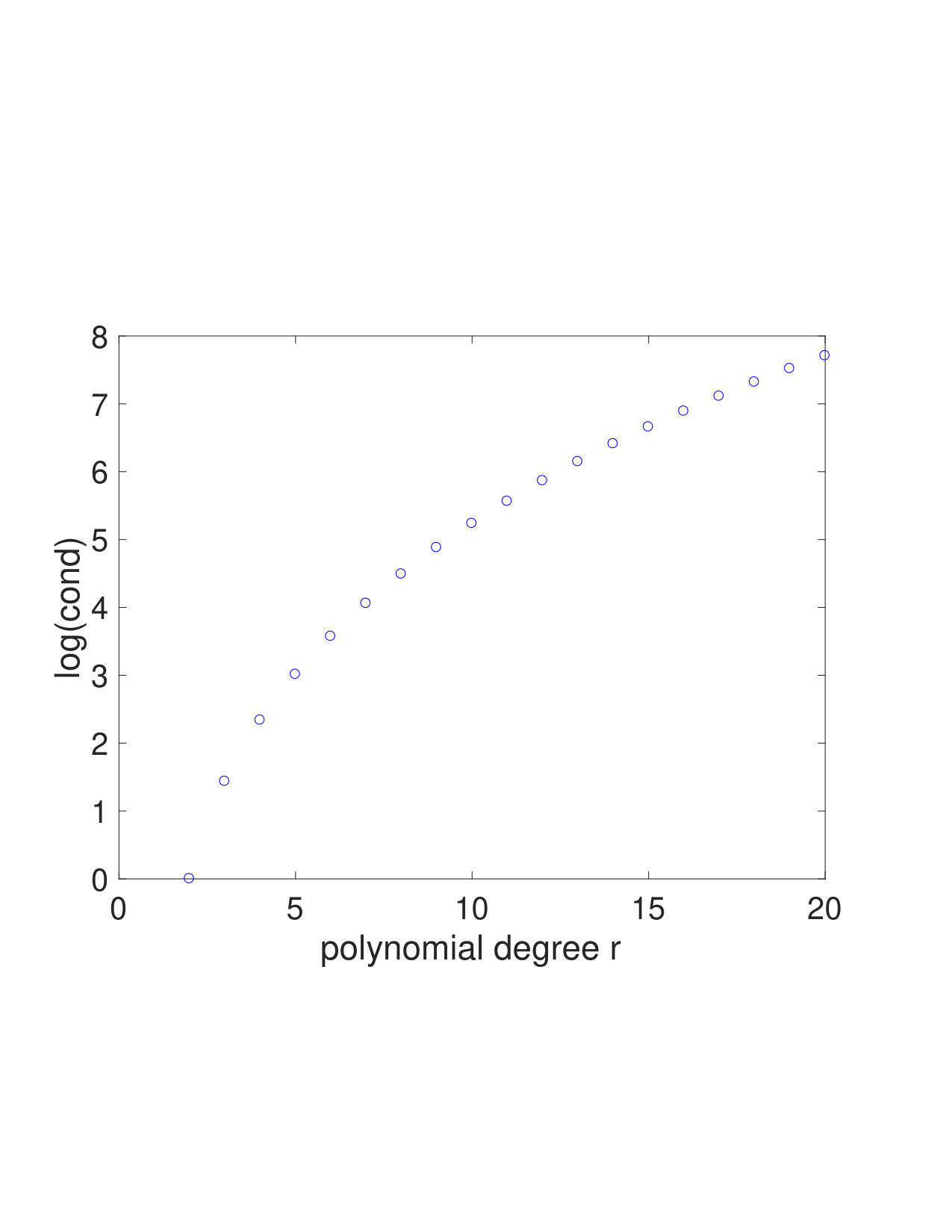 Figure 1
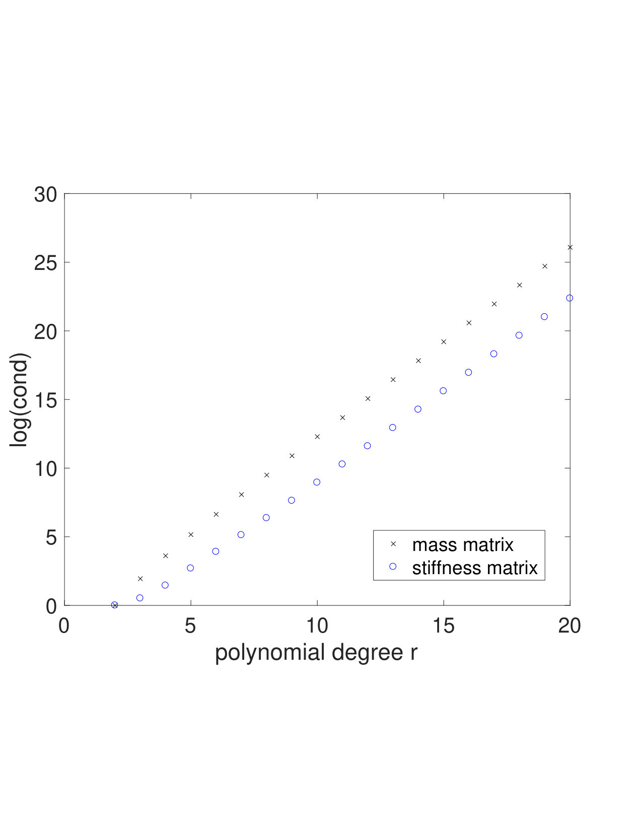 Figure 2
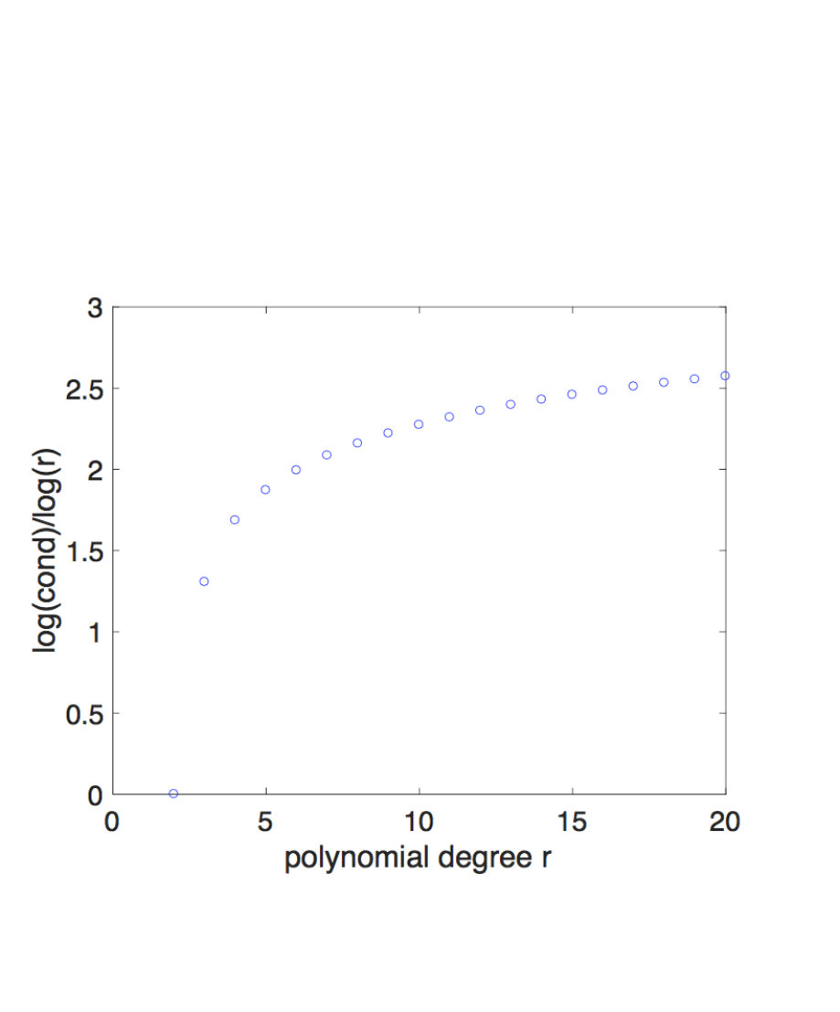 Figure 3
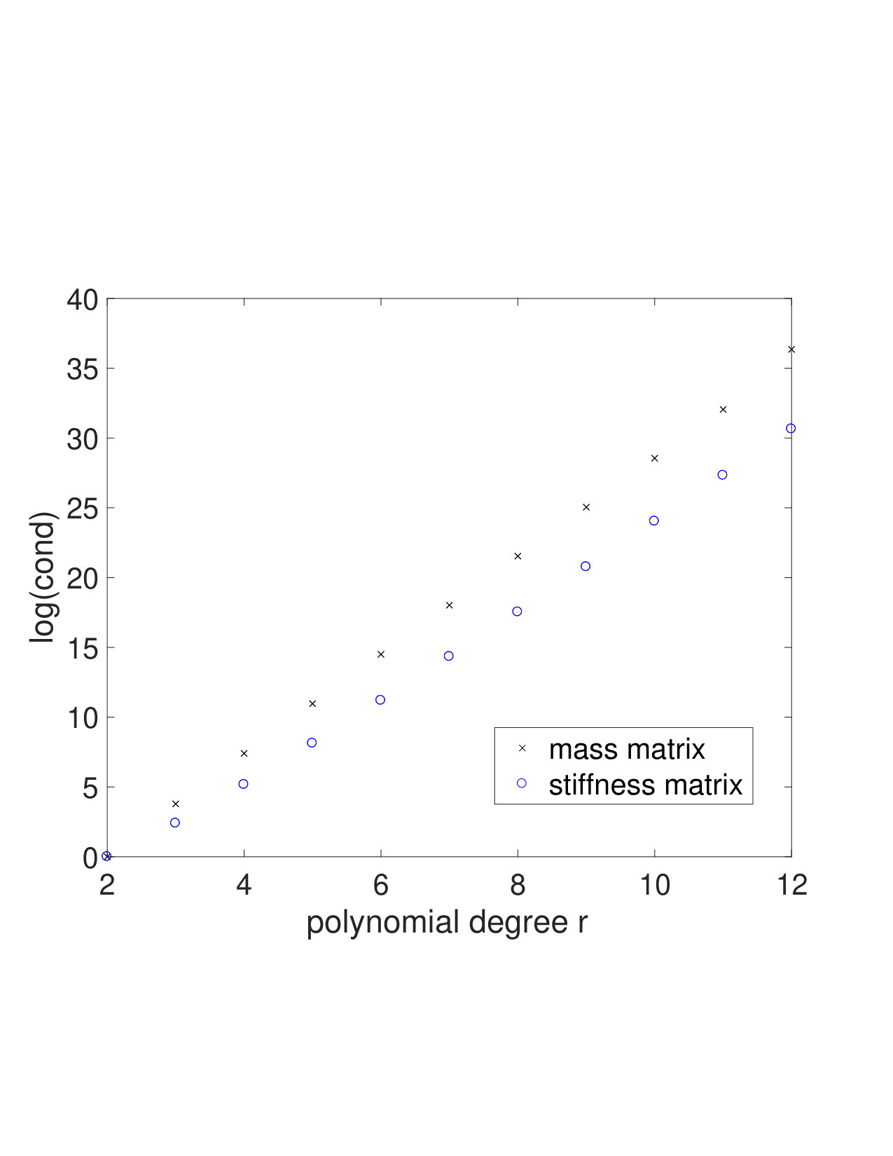 Figure 4
| r | 3 | 5 | 7 | 9 |
|---|---|---|---|---|
| 6.623 | 6.819 | 6.893 | 6.930 | |
| 0.427 | 0.457 | 0.472 | 0.481 | |
| cond. num. | 15.503 | 14.922 | 14.600 | 14.414 |
| dim. of frame | 33 | 98 | 199 | 336 |
| rank of frame | 19 | 46 | 85 | 136 |
| r | 3 | 5 | 7 | 9 |
|---|---|---|---|---|
| 6.624 | 6.819 | 6.893 | 6.930 | |
| 0.333 | 0.383 | 0.414 | 0.435 | |
| cond. num. | 19.869 | 17.809 | 16.647 | 15.929 |
| dim. of frame | 33 | 98 | 199 | 336 |
| rank of frame | 19 | 46 | 85 | 136 |
| r | 3 | 5 | 7 | 9 |
|---|---|---|---|---|
| 6.624 | 6.819 | 6.893 | 6.930 | |
| 0.348 | 0.396 | 0.427 | 0.446 | |
| cond. num. | 19.049 | 17.203 | 16.162 | 15.525 |
| dim. of frame | 73 | 222 | 455 | 772 |
| rank of frame | 43 | 106 | 197 | 316 |
Peer Reviews
No public reviews on file for this paper yet. If you reviewed it on a platform where reviews are public (OpenReview, ICLR, NeurIPS, ICML), you can paste yours below so the community can read it here.
Videos
No videos yet. Explain this paper in a talk, walkthrough, or lecture? Add one.
Taxonomy
TopicsAdvanced Numerical Methods in Computational Mathematics · Advanced Numerical Analysis Techniques · Numerical methods in engineering
Well-conditioned frames for high order finite element methods
Kaibo Hu
School of Mathematics, University of Minnesota, 55455 Minneapolis, MN, USA
[email protected] http://www-users.math.umn.edu/ khu/ and
Ragnar Winther
Department of Mathematics, University of Oslo, 0316 Oslo, Norway
[email protected] http://www.mn.uio.no/math/personer/vit/rwinther/index.html
Abstract.
The purpose of this paper is to discuss representations of high order finite element spaces on simplicial meshes in any dimension. When computing with high order piecewise polynomials the conditioning of the basis is likely to be important. The main result of this paper is a construction of representations by frames such that the associated condition number is bounded independently of the polynomial degree. To our knowledge, such a representation has not been presented earlier. The main tools we will use for the construction is the bubble transform, introduced previously in [5], and properties of Jacobi polynomials on simplexes in higher dimensions. We also include a brief discussion of preconditioned iterative methods for the finite element systems in the setting of representations by frames.
Key words and phrases:
Key words : high order method, finite element method, condition number, frame
1. Introduction
The discussion in this paper is motivated by finite element discretizations of second order elliptic equations, where piecewise polynomial spaces of high polynomial degree are used as the finite dimensional space. As the polynomial degree increases the choice of basis can have a substantial effect on the conditioning of the linear systems to be solved. The purpose of this paper is to discuss how to obtain representations of the finite element spaces which are uniformly well-conditioned with respect to the polynomial degree. Here the conditioning of the representation is measured by the condition number. Furthermore, we will explain how this influences the conditioning of the corresponding discrete systems. Since our main goal is to discuss dependence with respect to the polynomial degree we will consider the mesh to be fixed throughout the discussion below.
To motivate the discussion below, we consider a second order elliptic equation, defined on a bounded domain , which admits a weak formulation of the form:
Find such that
[TABLE]
where denotes the Sobolev space of all functions in which also have all first order partial derivates in . Furthermore, is a bounded linear functional, and is a symmetric, bounded, and coercive bilinear form on . The formulation above reflects that we are considering an elliptic problem with natural boundary condition. If we instead consider problems with an essential boundary condition on parts of the boundary, we will obtain a weak formulation with respect to a corresponding subspace of . However, the effect of such modifications of (1.1) will have minor effects on the discussion below. Therefore, we will restrict the discussion to problems of the form (1.1) throughout this paper.
A discretization of the problem (1.1) can be derived from a finite dimensional subspace of . In the finite element method is typically a space of piecewise polynomials with respect to a partition, or a mesh, , with global continuity, and where the mesh parameter indicates the size of the cells of the partition. The corresponding discrete solution is defined by:
Find such that
[TABLE]
This system can alternatively be written as a linear system of the form , where , and where the operator is defined by for all . Hence, is symmetric in the sense that for all , where is the duality pairing between and . To turn the discrete system (1.2) into a system of linear equations, written in a matrix/vector form, we need to introduce a basis for the space . This means that any element can be written uniquely on the form . We denote the map from to given by for . In a corresponding manner we define by . We note that if and then
[TABLE]
where is equipped with the standard Euclidean inner product, and where we adopt the standard “dot notation” for this inner product. Hence, can be identified as . If is the unknown vector, , then the system (1.2) is equivalent to the linear system
[TABLE]
where corresponds to the matrix representing the operator . The matrix is usually referred to as the stiffness matrix, and the element is given as . Furthermore, we note that the diagram
[TABLE]
commutes. However, there is a striking difference between the operator and its matrix representation . The stiffness matrix depends strongly on the choice of basis, while the operator only depends on the bilinear form and the space .
For piecewise polynomial spaces of high order the choice of basis can have dramatic effect on the conditioning of the stiffness matrix . Therefore, there are a number of contributions in the literature discussing how to choose proper bases for piecewise polynomial spaces of high order. The purpose of these constructions is usually motivated by the desire to control specific condition numbers or to control the sparsity of the resulting matrices. Let be the Riesz map given by
[TABLE]
The operator is symmetric and positive definite in the inner product. This operator is also basis independent, and its eigenvalues are given by the generalized eigenvalue problem
[TABLE]
If is the polynomial degree then its spectral condition number, , generally may grow like , cf. [1, 7, 16]. Therefore, one possiblity is to design a special basis such that the spectral condition number of the stiffness matrix is much smaller than that of the operator , i.e.,
[TABLE]
The obvious constructions which will lead to this is to consider bases which are close to orthonormal with respect to the bilinear form . This approach is taken by Schwab in [16], where integrated Legendre polynomials are used to construct a basis in one space dimension. However, the generalization of this approach to higher dimensions is not obvious. Babuška and Szabó [17] used these basis functions in a tensor product setting to obtain bases for cubical meshes in higher dimensions. In [7] it is established that for such bases one has an estimate for the condition number of the stiffness matrix of the form , while , where is the mass matrix given by and is the space dimension. In particular, these estimates indicate that in higher dimensions it may occur that is much larger than its basis independent counterpart, . Similar constructions on triangular and tetrahedral meshes are based on orthogonal polynomials with respect to triangles and tetrahedrons constructed by the Duffy transform, i.e., mappings between simplexes and cubes, cf. [2, 6, 8, 11, 22]. In a slightly different direction, Xin and Cai [19] used multivariate orthogonal polynomials on simplexes to design hierarchical bases for the discontinuous Galerkin method.
Our aim in this paper is to construct representations of finite element spaces with condition numbers which are bounded independently of the polynomial degree. If the spaces are represented by a basis this quantity can also be characterized as the spectral condition number of the mass matrix. We will argue below that if is well-behaved then the condition number of the stiffness matrix is basically controlled by the basis independent quantity , cf. (2.2) below. In fact, we will not restrict the discussion below to bases, but instead also allow representations of finite element spaces by frames, i.e., generating sets with redundancy. This more general set up allows us to identify a construction which will lead to representations with condition numbers which are independent of the polynomial degree . The key tools we will use for this construction include the properties of the bubble transform, cf. [5]. By combining proper results for the bubble transform with general results for frames based on space decompositions, the construction of frames with condition numbers bounded independently of the polynomial degree is reduced to a pure polynomial problem. More precisely, we need to construct Jacobi polynomials on standard simplexes in higher dimensions, and these constructions are well known, cf. [4].
The rest of this paper will be organised as follows. In Section 2, we will present some notation and preliminaries needed for our discussions. In particular, we present a simple bound that relates the spectral condition number of the stiffness matrix and the mass matrix, and we present some elementary numerical examples to illustrate the sharpness of this bound. Furthermore, we will recall the construction of the bubble transform and its properties. Section 3 is devoted to a discussion of frames obtained by a space decomposition, where we focus on general estimates for the appropriate condition numbers. The construction of the specific frames are completed in Section 4, where we explain how to utilize well-conditioned bases on local subdomains. We focus on the construction of orthogonal local bases in Section 4 and present explicit forms of the local bases based on Jacobi polynomials on simplexes. We present numerical experiments based on these local constructions which give results that are consistent with the theory. In particular, the results of the experiments indicate that the behavior of the frame condition numbers are robust with respect to perturbations of the mesh, even when the mesh is nearly degenerate. Sections 5 is devoted to the discussion of preconditioned Krylov space methods for the associated frame systems, which in general will be singular. In particular, we make the observation that under the assumption of standard representations of the discrete elliptic operator and the preconditioner, the conditioning of the preconditioned system is, in a proper sense, independent of the choice of basis or frame. On the other hand, the representation will substantially effect the individual conditioning of the stiffness matrix and the matrix representation of the preconditioner. However, we will argue that as long as the condition number of the representation stays bounded, then these matrices will roughly behave like their basis independent counterparts. Finally, some concluding remarks are given in §6.
2. Notation and preliminaries
We assume that is a bounded polyhedral domain in . We recall the definition of the Sobolev spaces
[TABLE]
and the corresponding subspace of functions with vanishing trace:
[TABLE]
We assume that is a simplicial mesh on . If is a subset of we let denote the polynomials with degrees less than or equal to on , while the corresponding space of -piecewise polynomials with respect to the mesh is denoted , i.e.,
[TABLE]
2.1. Representation of discrete operators
Consider a finite element system of the form (1.3), where the space for a suitable , and let be any basis for . We recall that the stiffness matrix is given as , where is the discrete elliptic operator defined by the variational problem (1.2). The corresponding mass matrix is the matrix with elements . Alternatively, , where we recall that is the Riesz map, mapping to . The matrices and are related by the relation
[TABLE]
We note that the operator is similar to the basis independent operator . A direct consequence of the identity (2.1), using the characterization of the extreme eigenvalues by the Raleigh quotient, is the inequality
[TABLE]
where the spectral condition number is basis independent, while is independent of the underlying elliptic operator. In fact, (2.2) follows from the stronger properties
[TABLE]
where and denote the extreme eigenvalues. To see this just observe that
[TABLE]
and a similar argument establishes the corresponding inequality for .
We can therefore conclude that if the basis is chosen such that is properly bounded, then the conditioning of the stiffness matrix is no worse than its basis independent analog. To illustrate the effect on the conditioning of the stiffness matrix , by controlling the condition number of the basis, we present some simple numerical examples in one space dimension. In other words, we are testing the sharpness of the bound (2.2) in the simplest possible setting.
Example. We consider the Laplace problem in one space dimension, with homogeneous Dirichlet boundary conditions, i.e., the bilinear form is given by
[TABLE]
and we use a mesh consisting of one interval. Therefore, the corresponding spaces will be given as , where is the interval and is the space of polynomials of degree on which vanish on the boundary. We will investigate the effect of choosing three different bases for the spaces , by computing the condition numbers of the mass matrix , the stiffmess matrix and the condition number of the basis independent operator . In fact, for any basis the latter is equal to .
Our first test is based on an orthonormal basis. We consider the polynomials , where is the orthonormal Jacobi polynomials on with respect to the weight , i.e.,
[TABLE]
cf. Appendix A below. Since these polynomials form an orthonormal basis for for all and . The logarithms of the latter, for increasing values of , are shown in Figure 2, while are compared to in Figure 2. The growth depicted here is consistent with the asympotic upper bound, , cf., [1].
Next we consider the Bernstein basis. More precisely, for any consider the functions , where The condition numbers of the mass and stiffness matrices are shown in Figure 4, and the results indicate that both and grow exponentially with . This is consistent with the explicit formula, , which holds in the case of no boundary condidtions [3, 12]). Furthermore, we observe that is several magnitudes larger than the basis independent quantity
Finally, we consider the corresponding power basis . The condition numbers of the mass and stiffness matrices are in this case even much larger than for the Bernstein basis, cf. Figure 4. Due to the extremely bad condition numbers, the computations are only reliable for small values of .
The experiments just presented illustrate an effect of the bound (2.2). For the Jacobi basis the condition number of the mass matrix is well controlled, and as a consequence the growth of is moderate. On the other hand, for the two other bases and both grows much faster than
2.2. The local spaces
The rest of this paper will mostly be devoted to the construction of representations for the spaces which admit condition numbers which are independent of the polynomial degree . To obtain such a result we will not restrict the discussion to representations by bases, but we will allow more general representations by frames. In particular, our construction will rely on results for the bubble transform derived in [5]. To present these results, and to explain how they will be used here, we will first introduce some additional notation.
If is simplicial triangulation of , we let be the set of all the subsimplexes of of dimension , while contains all the subsimplexes. If we let be the set of all subsimplexes of . For , the local patch, or macroelement, is the union of all the elements of the mesh which contains . Furthermore, is the partition restricted to .
When is a vertex, we use to denote the piecewise linear function which equals one at , and equals zero at other vertices. From another point of view, is the barycentric coordinate associated to , extended by zero outside the macroelement . For and , i.e. the convex hull of vertices , we use to denote the vector field . Following the approach taken in [5] we will consider as a mapping from the domain to the standard simplex in given by
[TABLE]
We also define to be the face of opposite the origin, i.e,
[TABLE]
such that , i.e., is the set of all convex combinations of the origin and elements of . The mapping , restricted to , is surjective but not injective (see Figure 5 for the case ).
If then the associated macroelement can be characterized as , while the corresponding extended macroelement, , is defined by
[TABLE]
The pull back of the extended barycentric coordinates, , given by
[TABLE]
maps functions on to functions on which are constant and equal to outside . Furthermore, if then vanishes on the boundary of .
The space of polynomials of degree less than equal to which vanish on will be denoted , i.e.,
[TABLE]
By applying the pullback, , to this polynomial space we obtain
[TABLE]
The elements of this space are polynomials in the variables , and they vanish on the boundary of . In other words, the space can be identified with a subspace of , the subspace of which consists of functions which vanish on . In fact, in the special case when , i.e., when we define the to be equal to . Alternatively, if we define to be for , then the identification (2.3) also holds in this case. The local spaces will act as key building blocks in our construction below.
2.3. The bubble transform
The bubble transform is a map that depends on the mesh , but no piecewise polynomial space occurs in the definition. In particular, it does not depend on a degree parameter . In [5] the construction of the bubble transform was partly motivated by the desire to design local projections onto the piecewise polynomial spaces with proper bounds independent of . In this paper, we will utilize the properties of the bubble transform to construct frames for the spaces that admit condition numbers which are independent of the degree parameter .
The bubble transform is a map of the form
[TABLE]
It is a tool to decompose an function defined on into components with local support in . More precisely,
[TABLE]
where
[TABLE]
gives the component of which is supported on . In particular, we observe that the operator is local in the sense that depends on . Another key property of the map is that it is invariant with respect to the piecewise polynomial spaces , i.e., if then .
The bubble transform has a recursive definition. We briefly recall its construction, but for more details we refer to [5]. For , is of the form
[TABLE]
where
[TABLE]
while if . The pull back , mapping functions on to functions on , is discussed above. The operator is an average operator, while is refereed to as a cut-off operator. If then for any
[TABLE]
where is given by
[TABLE]
The operator maps a function defined on to a function defined on , and it is a smoothing operator in the sense that for any the function will have point values away from the simplex . On the other hand, corresponds exactly to . Furthermore, the operator has the property that it maps piecewise polynomials into polynomials. More precisely, if then .
The cut-off operator maps the set of functions defined on to itself. Its key property is that it preserves the trace on , i.e., , while it kills the trace on the rest of the boundary of , i.e, . In addition, is polynomial preserving in the sense that if , with , then .
The key properties of the bubble transform are stated in [5, Section 4]. For the convenience of the readers, and since most of these properties are essential for the discussion below, we summerize the main results here.
- (1)
The construction using barycentric coordinates: For and
[TABLE]
where is defined by (2.4), while if . 2. (2)
The boundedness in and :
[TABLE]
where is a generic constant not depending on the function . 3. (3)
Partition of unity: If then 4. (4)
Local support: If then . 5. (5)
Polynomial preserving: If then
We also note that if , where then
[TABLE]
where the constant only depends on the number of overlaps of the subdomains . Therefore, by combining this with (2.5) we obtain that the norms and are equivalent.
The bubble transform suggests a decomposition of the finite element spaces of the form
[TABLE]
In fact, this decomposition follows directly from the properties above. The spaces are local spaces consisting of piecewise polynomials with support on . On the other hand, the sum above is in general not direct. To see this, we observe that that if is a vertex, i.e., then
[TABLE]
where is the extended barycentric coordinate of the vertex . In particular, the function is an element of for . Let be the other vertices in with correponding exteded barycentric coordinates . Then the function can alternatively be expressed as
[TABLE]
Furthermore, , where . We conclude that the function is both in and , and therefore the sum (2.7) is not direct. Similar redundancies also appear for the spaces for simplices of higher dimensions. Therefore, if we want to utilize the decomposition (2.7), and bases for the local spaces , to represent the functions in the spaces we are forced to study representations by frames.
Interpreting the properties of the bubble transform for the decomposition (2.7) of the following result is obtained.
Theorem 2.1**.**
The decomposition (2.7) is stable in the sense that there exists , and a positive constant such that
[TABLE]
Furthermore, as a result of the finite overlapping property of the mesh topology, there exists a positive constant such that
[TABLE]
3. Estimates of frame condition numbers
We will utilize the decomposition (2.7) to obtain a well conditioned representation of functions in the space . More precisely, we will combine the decomposition (2.7) with a basis for each of the spaces . Due to the redundancy of the decomposition (2.7) this will lead to a spanning set for the functions in where the elements are not linearly independent, i.e., we obtain representations by frames, cf. [14]. Therefore, we will give a brief review of representations by frames. In particular, we will discuss frames obtained from space decompositions.
Throughout this section we use to denote a real, finite dimensional Hilbert space with inner product . Roughly speaking, a frame is a set of generators which allow redundancy. In other words, if then each element can be expressed as a linear combination , but this representation is in general not unique. The condition number of the frame , , is defined as
[TABLE]
where
[TABLE]
In other words, and are the optimal constants such that the bounds
[TABLE]
holds. Therefore, is the natural concept to relate the norm of to the norm of its coefficients measured in .
Remark 1**.**
If is a basis then it is well known that is equal to the spectral condition number of the corresponding “mass matrix,” with elements . In fact, the parameters and , given in (3.1), are exactly the smallest and largest eigenvalue of the mass matrix. In the case of a frame, the mass matrix will in general be singular. In this case is still the largest eigenvalue of the mass matrix, while is the smallest positive eigenvalue.
In fact, a similar characterization can be given in the case of frames, cf. Section 5.2 below.
3.1. Frames based on space decomposition
To give a general description of frames based on space decomposition, we assume that the space admits a decomposition of the form
[TABLE]
where are subspaces of . The decomposition is not assumed to be direct, but we assume that there exists a positive constant such that for any , we have
[TABLE]
Furthermore, we assume that there is a positive constant such that all admits a decomposition , , where
[TABLE]
Of course, due to (2.5) and (2.6), these bounds are known to hold for the spaces with inner product. We will use the decomposition (3.2) to define a frame for . More precisely, for each let be a basis for the space . The frame is then given as , where is the dimension of . For each we assume that are the optimal constants such that
[TABLE]
In other words, is the condition number for the basis of .
Theorem 3.1**.**
Assume that the decomposition (3.2) satisfies (3.3), (3.4) and (3.5). The frame introduced above satisfies
[TABLE]
Proof.
Let and be the two constants defined by (3.1). We will show that
[TABLE]
From these bounds we immediately obtain
[TABLE]
which is the desired bound. Therefore, it is enough to establish the bounds given by (3.6).
To show the first inequality, let be any element in , and a decomposition of the form (3.2) satisfying (3.4). Furthermore, let be the unique coefficients such that . Then
[TABLE]
This implies
[TABLE]
and the first inequality of (3.6) follows by taking infimum over all elements of of .
On the other hand, for any coefficient , we define and . We then have
[TABLE]
Therefore, for any , we have
[TABLE]
and hence the second bound of (3.6) follows. ∎
The result above shows that the condition number of the frame is bounded by the constants and , derived from the decompostion (3.2) and the local condition numbers . In addition, the factor , which we will refer to as a scaling factor, appears. This factor will be small if all the local condition numbers are small, and if the local bases in addition are scaled similarly. In fact, the appearance of this factor is similar to a well known phenomenon. Consider a block diagonal matrix of the form
[TABLE]
where and are identity matrices of proper dimensions, and where is a real parameter. Then each block has condition number , while the full matrix has condition number due to the different scaling of the two blocks.
3.2. The bubble decomposition of
We end this section by applying Theorem 3.1 to the decomposition (2.7) of the spaces . For each let denote the dimension of the space . We will see below that it is possible to construct a basis for each of the spaces such that all are well conditioned in , and with a comparable scaling. Therefore, consider the set up when we have a basis for each of the spaces of the form , satisfying
[TABLE]
where the positive constants and are independent of . By combining Theorem 3.1 with Theorem 2.1 we immediately obtain the following.
Corollary 3.1**.**
Let be the frame representation of the space just introduced, and satisfying (3.7). We have the estimate:
[TABLE]
where and are the constants appearing in (2.5) and (2.6).
Proof.
It is a consequence of (3.7) that the condition number of each local basis, of , is bounded by , and that the same bound holds for the scaling factor appearing in Theorem 3.1. The result therefore follows from this theorem. ∎
Remark 2**.**
We note that in the special case when each of the local bases is orthonormal then the bound above reduces to , i.e, the condition number of the frame is bounded entirely by the two constants given in (2.5) and (2.6).
4. Construction of bases for the local spaces
Based on the discussion above, cf. Corollary 3.1, we can conclude that to obtain a well-conditioned frame for the spaces , it is enough to construct bases for the local spaces which are uniformly well-conditioned in . More precisely, it is enough to construct bases for the spaces such that condition (3.7) holds. In the special case when then , and the construction of a basis for this space is well known. We return to this case in the Appendix below. When we recall from Section 2 that is defined by a pull back, with respect to the map , of the polynomial space , where is a reference simplex in and . Therefore, we will construct a basis for the space by utilizing a basis for .
4.1. Construction of local bases
Element of the space is of the form , where . Therefore, any basis for the space leads to a corresponding basis for . To proceed we recall the fact from [5, formula (5.6)], that if is any smooth function on then
[TABLE]
where , and is a scaling factor depending on the geometry of the macroelement . In fact, in the notation of [5, Section 5] the constant is given by
[TABLE]
where is a piecewise flat manifold of dimension contained in , and is a piecewise constant function on . However, for the discussion here it suffices to observe that , uniformly with respect to a family of shape regular meshes. Here is a local parameter representing the diameter of , i.e. represents the size of the elements contained in . As a consequence, if and are orthogonal functions on , with respect to the weight functions , then and are orthogonal functions on . Alternatively, if and are elements of , which are orthogonal with respect to the weight function , then the corresponding functions and are orthogonal functions belonging to the space . Furthermore, the norm of in is equivalent to times the corresponding weighted norm of on . Therefore, the problem of constructing orthogonal and uniformly scaled bases for the local spaces , is equivalent to the construction of bases for the polynomial spaces , which are orthogonal with respect to the weight function , and uniformly scaled. Actually, since the scaling factor only depends on and is uniform for all the bases associated with , any orthonormal bases on with the weight will transform to bases of with condition number one.
To construct a polynomial basis, which is orthogonal with respect to a polynomial weight function, corresponds to the study of Jacobi polynomials. Single variate orthogonal polynomials are of course well studied, but there are also explicit formulas for Jacobi polynomials with respect to simplexes in higher dimensions. The most popular approach to construct orthogonal polynomials in higher dimensions is to use a transform between simplexes and cubes, referred to as “the Duffy transform” or “the Koorwinder method” [9]. Furthermore, hierarchical constructions of orthogonal polynomial can be found in [4].
4.2. Numerical results
As an example, we present explicit formulas of our frames and explore the condition numbers of the matrices by numerical computation. This will verify our theoretical results and show that the frame is well-conditioned and the constants and in (3.8) are bounded on various regular or irregular meshes. We will only consider the two dimensional case, i.e., the space dimension is equal to .
Let be the standard single variate Jacobi polynomial of degree with weight defined on (see also Appendix below). Define
[TABLE]
so that is a single variate orthogonal basis on with weight . The explicit formula for our frames are derived from the corresponding basis for the spaces for , cf. (2.3), where we recall that . Let be the barycentric coordinates of extended to . The explicit bases for the spaces can be given as follows:
[TABLE]
for the three cases . In fact, these functions are special cases of the simplicial orthogonal polynomials (6.2), cf. the Appendix below. The corresponding bases for the spaces are given by (2.3) for . We note that the functions in (4.3) and (4.4) do not have rotational symmetry, meaning that exchanging two barycentric coordinates in the formulas will lead to different bases. In the assembling of matrices permuting the variables in (4.3) may facilitate the match of orientation.
To avoid considering effects from inaccurate numerical quadrature, in the computation we use Gauss type formulas on triangles with order 20 [23]. Since in the tests below we only consider polynomials of degree less than 10, the numerical quadrature will lead to exact integration. Due to the roundoff error, the mass matrices of the frames do not have precise zero eigenvalues. Therefore we will use a tolerance to select nonzero eigenvalues and thus will consider all numbers near the machine precision as zero.
The bases of defined above are orthogonal on each triangle of . Therefore the block of the mass matrix corresponding to contributions from a single macroelement is diagonal on each triangle. This is also observed in the numerical tests below. However, bases associated to different macroelements can still interfere with each other and the contribution of this overlapping effect to the condition number is reflected in the bound (3.8) with constants and .
In the numerical tests below we consider the mass matrix in the case when the complete mesh is a single vertex macroelement. Alternatively, this matrix can be thought of as a ”local block matrix” of a mass matrix generated by a larger mesh. On this local mesh we consider all the frame functions generated by all the subsimplexes of the mesh. In all the examples below the local mesh corresponds to the macroelement of the origin, and we will consider three cases:
- •
Test 1: a macroelement consisting of three triangles with boundary vertices (1, -1), (0, 2), (-1, -1) (left of Figure 6);
- •
Test 2: distortion of Test 1, which has three triangles with boundary vertices (1.3, -0.0001), (0, 2.12), (-1, -0.0001) (right of Figure 6);
- •
Test 3: a macroelement consisting of six triangles with boundary vertices , , , , , , (Figure 7).
The diagonal entries of the mass matrix are scaled to one such that the bases are scaled to have unit norms. In the tables below, dimension of the frame means the number of functions in the frame representation, while rank of the frame means the rank of the mass matrix. Alternatively, the rank of the frame can be identified as the dimension of the space of continuous piecewise polynomial of the same degree on the same mesh.
The condition numbers in Test 1 are shown in Table 1. Here denotes the minimal nonzero eigenvalue. Due to the roundoff error, the minimal nonzero eigenvalue slightly decreases as increases, in contrast to the monotonicity predicted by the min-max principle. Thus the condition numbers also slightly decrease.
The results on a distorted mesh, Test 2, are shown in Table 2. The condition numbers are only slightly larger than those in Test 1, showing that the condition numbers are nicely bounded even if there are very thin elements present in the mesh.
The results for Test 3 are shown in Table 3. Similar to Test 1 and 2, the condition number also remains bounded as the degree increases.
Patterns of the mass matrices, i.e., the zero–nonzero structure, are shown in Figure 9 and Figure 9 for Test 1. The pattern only depends on the ordering of the bases and the topology of the mesh. Therefore, the results for Test 1 and Test 2 are the same. In the results below the bases are in the order of the interior vertex, boundary vertices, boundary edges, interior edges and finally interior modes. The corresponding results for Test 3 are given in Figure 11 and Figure 11. Due to the locality of the frames, more sparsity appears as the mesh has more triangles.
5. Iterative methods and preconditioning
We recall the setting discussed in the introduction of this paper, where is a piecewise polynomial space. In the first part of this paper we have outlined how to construct representations of the spaces by frames which admit condition numbers which are bounded independently of the polynomial degree. The main purpose of this section is to present a brief discussion of the use of preconditioned iterative methods in the setting of representations by frames. In particular, we will clarify how the preconditioned iteration is effected by the boundedness of the condition number. However, before we discuss this in the setting of frames we will first review the more standard situation when the computation relies on a basis for the space .
5.1. Representation by a basis
If is a basis for the space , then the two bijective maps and , introduced in Section 1, are used to represent elements of and , respectively. The stiffness matrix admits the representation , where the operator is independent of the choice of basis. Discrete elliptic systems of the form (1.2), or equivalently (1.3), are most effectively solved by preconditioned iterative methods. Therefore, it seems appropriate to study the effect of the choice of basis on the complete preconditioned system.
In operator form the preconditioned system appears as
[TABLE]
where the preconditioner is an operator, , which is symmetric and positive definite with respect to the duality pairing between and . Furthermore, its standard representation is the matrix . The two basic necessary conditions for the construction of an effective preconditioner are, i) the spectral condition number of is well behaved, and ii) the matrix-vector products of the form , for any , can be evaluated fast. Since the stiffness matrix usually is represented by a sparse matrix, the second condition will hold if the matrix-vector products of the form can be evaluated fast. It is not the purpose of this paper to discuss the design of effective preconditioners. Instead we refer to [13, 20, 21] for general discussions of such constructions. Our main concern here is to discuss how the condition number of the basis influences the key properties of the preconditioned iterative method.
The convergence of a standard iterative method for the preconditioned system, such as the conjugate gradient method, will be governed by the spectral condition number of the coefficient matrix,
[TABLE]
However, this matrix is similar to the operator , and therefore its condition number is independent of the basis. On the other hand, the basis will effect the properties of the two matrices and . These operators have to be evaluated in each iteration, and their conditioning will effect the numerical stability of the computations. Recall the inequality (2.2), which relates , and the condition number of the basis, . In fact, is the only quantity on the right hand side of the inequality (2.2) which is basis dependent. Furthermore, the numerical experiments presented in Section 2 indicate that this inequality is rather sharp. Therefore, if the mass matrix is well-conditioned then will behave approximately like the basis independent condition number . This condition number reflects the properties of the elliptic operator we are approximating.
The situation for the preconditioner is similar. The matrix admits the representation
[TABLE]
and from this we can easily derive the inequality
[TABLE]
Therefore, if the mass matrix is well conditioned, then we can conclude that is essentially bounded by a basis independent quantity. We have therefore seen that, even if the choice of basis has no direct effect on the conditioning of the preconditioned system, an well-conditioned basis will result in matrix representations and with condition numbers that roughly behave like their basis independent counterparts. Below we will argue that these conclusions also hold if we allow representations by frames.
5.2. Representations by frames
Assume that we are given a frame of , where in general is larger than the dimension of . The operators and , are defined as above, i.e.,
[TABLE]
such that the identity holds. In this setting the operator is surjective, the operator is injective, and as above and correspond to the dual of the other. If the condition number of the frame, , is controlled then we will argue that also in this case the matrix representations of the discrete elliptic operator and suitable preconditioners behaves roughly like the corresponding basis independent counterparts. In fact, this simply follows by proper block decompositions of the matrices.
The stiffness matrix, representing the coefficient operator is still defined as , cf. (1.4). While the operator is positive definite, the stiffness matrix is only positive semi-definite with and
[TABLE]
Here the orthogonal complement is with respect to the standard Euclidean inner product of . In fact, with respect to the orthogonal decomposition the matrix has a block structure of the form
[TABLE]
where the matrix is a positive definite matrix on . The mass matrix, , with elements , has a similar block structure of the form
[TABLE]
with respect to the decomposition . Here the the matrix , mapping into itself, is positive definite. Furthermore, it follows from the observation done in Remark 1 that . The marices and can be related by the identity
[TABLE]
where denotes the restriction of to . By arguing as above, this leads to
[TABLE]
which is a generalization of inequality (2.2). Therefore, we can again conclude that behaves roughly like its basis independent counterpart, , as long as the frame condition number is well controlled.
In the setting of frames a preconditioner is represented by an matrix which is symmetric and positive definite with respect to the Euclidean inner product. Furthermore, the corresponding operator is given by the diagram
[TABLE]
i.e., . The operator is symmetric in the sense that for ,
[TABLE]
and is positive definite since has this property. Furthermore, the identity
[TABLE]
holds. We will implicitly assume that has an interpretation as an operator from to which is independent of the choice of frame. In this respect, also the operator , and its spectral condition number, will be frame independent. In fact, we will justify this assumption in Section 5.3 below, in the case when the frame is derived from a basis of each of the local spaces , cf. (2.7).
Consider a linear system of the form (1.2), i.e., , where the data and . The preconditioned version of this system takes the form
[TABLE]
or in matrix-vector form
[TABLE]
where is any vector such that . Hence, even if the solution is uniquely determined by the system, the vector is only determined up to addition of elements in .
It is well known that Krylov subspace methods can be used to solve semidefinite systems, cf. for example [10]. In fact, if we consider a system of the form (5.7), with initial guess , then the initial residual
[TABLE]
where the superscript indicates orthogonality with respect to the inner product generated by the positive definite matrix . The matrix maps to itself, and as consequence all the vectors in the associated Krylov spaces, spanned by vectors of the form , will be in this space. As a consequence, we can view the iterative method as if it is restricted to the space , where the system (5.7) has a unique solution. Furthermore, the convergence rate will be bounded by the spectral condition number of the coefficient matrix restricted to this space. If we let be the restriction of to then is invertible and from (5.5) we obtain
[TABLE]
as a generalization of the similarity relation (5.1). In particular, this shows that the spectral condition number of the matrix , restricted to , is equal to the spectral condition number of the operator . Therefore, also in the case of representations by frames, we can conclude that the performance of a preconditioned Krylov space method is, in a proper sense, independent of the choice of representation of the spaces and . However, as we have seen above, a well condition frame guarantees that the conditioning of the stiffness matrix reflects the condition number of its basis independent counterpart, cf. (5.4). A similar conclusion for the preconditioner, i.e., a generalization of inequality (5.3), is also easily established.
5.3. Representation of the preconditioner
The discussion above is based on the assumption that the matrix , representing the preconditioner , is positive definite, and that the operator has an interpretation which is independent of the representations of the spaces and . Here we will argue that if is of the form and the frame is generated by an overlapping decomposition of the form (2.7), then this assumption is indeed very natural. To illustrate this we consider an additive Schwartz preconditioner of the form proposed in [15]. In operator form this preconditioner has the structure
[TABLE]
where is a “coarse space preconditioner”, and are local preconditioners defined with respect to local spaces . More precisely, each of the operators are preconditioner for the corresponding local operator defined by the bilinear form with respect to the local space , while is a corresponding preconditioner defined with respect to the piecewise linear space .
Consider the set up in Section 3.2 above, where for each the set is a basis for the local space , and . The natural representations of the operators are matrices of the form , where the representations and are defined as above, but now with respect to the local spaces . Furthermore, since is a basis for this space, each of the maps and is invertible, and as a consequence, the matrix is positive definite. The matrix , representing the preconditioner , will now be of the form
[TABLE]
where . Here is a symmetric and positive semidefinite matrix representing the operator , while the block diagonal matrix, , is symmetric and positive definite, since each block has this property. We refer to [15] for more details and tests of numerical performance.
Remark 3**.**
The additional global operator appears in the preconditioner proposed in [15] in order to obtain condition numbers which are independent of the mesh size . In the present paper, where we consider the mesh to be fixed, we could have dropped this term and still obtain condition numbers which are bounded uniformly with respect to the polynomial degree .
6. Concluding remarks
The purpose of this paper is to discuss how to represent finite element spaces of high degree. More precisely, we study the spaces , consisting of piecewise polynomial spaces of degree with respect to a simplicial mesh . When the degree grows, the choice of basis for the spaces will intuitively affect the properties of the corresponding linear systems derived from a finite element discretization. The construction outlined in this paper, based on properties of the bubble transform and of Jacobi polynomials with respect to simplexes, leads to frames with condition numbers which are independent of the polynomial degree. In this respect, we have been able to present a procedure to construct well-conditioned frames. Furthermore, we have shown that such frames leads to stiffness matrices, and matrix representations of corresponding preconditioners, with condition numbers that behave roughly like their operator counterparts.
A possible disadvantage of a representation by a frame instead of a basis, is that the number of unknowns is increasing. For the frames proposed above the following table compares the dimension of the frame with a corresponding standard basis.
Basis Frame
1D
2D
3D
Here and are the number of vertices, edges, faces and 3D cells in the triangulation. We observe that even if the frame representations have redundancy, the asymptotic order of the total dimensions remains the same. Of course, in addition to condition numbers there are potentially a number of other criteria that could have been used to choose a basis or a frame, for example sparsity and fast evaluation of the stiffness matrix and the preconditioner. However, such discussions are outside the scope of the present paper.
Appendix. Jacobi polynomials on simplexes
The purpose of this appendix is to present precise formulas for basis functions of the local spaces . We will first consider the case when . We recall from Section 4 above that if we can construct bases for the polynomial spaces , which are orthonormal with respect to the weighted inner product with weight , then the corresponding set will be uniformly scaled bases for the spaces . Therefore, we will briefly outline how such bases for the spaces can be constructed. This discussion is based on multi-variate Jacobi polynomials on simplexes, and is mostly taken from [4, Section 5.3], cf. also [18] where the scaling of the polynomials is corrected.
We use to denote the orthonormal Jacobi polynomial on interval with weight , i.e.
[TABLE]
Using a linear transform , we get Jacobi polynomials on the reference interval :
[TABLE]
where
[TABLE]
We introduce the notation
[TABLE]
so that is a single variate orthogonal basis on with weight .
We define
[TABLE]
Given integer and , we will define a basis for the space . We consider the polynomials given by
[TABLE]
where is a multi-index. Here the constants and are given by and
[TABLE]
The polynomials (6.2) form a mutually orthonormal basis for with the weight .
For , the construction is similar and more standard. To construct a basis for , we can follow [4] to construct orthonormal bases for with weight . The set will be uniformly scaled bases for the spaces , where is defined by the barycentric coordinates.
Acknowledgments.
The authors are grateful to Douglas N. Arnold, Richard S. Falk and Jinchao Xu for several discussions about the results of this paper.
The research leading to these results has received funding from the European Research Council under the European Union’s Seventh Framework Programme (FP7/2007-2013) / ERC grant agreement 339643. The research of the first author leading to the results of this paper was partly carried out during his affiliation with the University of Oslo, partly supported by China Scholarship Council (CSC), project 201506010013.
The reference list from the paper itself. Each links out to its DOI / PubMed record.
- 1[1] Christine Bernardi and Yvon Maday. Spectral methods. Handbook of numerical analysis , 5:209–485, 1997.
- 2[2] Sven Beuchler, Veronika Pillwein, Joachim Schöberl, and Sabine Zaglmayr. Sparsity optimized high order finite element functions on simplices. In Numerical and Symbolic Scientific Computing , pages 21–44. Springer, 2012.
- 3[3] Z Ciesielskii and J Domsta. The degenerate b-spline basis as basis in the space of algebraic polynomials. Ann. Polon. Math , 26:71–79, 1985.
- 4[4] Charles F Dunkl and Yuan Xu. Orthogonal polynomials of several variables . Cambridge University Press, 2014.
- 5[5] Richard S Falk and Ragnar Winther. The bubble transform: A new tool for analysis of finite element methods. Foundations of Computational Mathematics , pages 1–32, 2013.
- 6[6] Thomas Führer, Jens Markus Melenk, Dirk Praetorius, and Alexander Rieder. Optimal additive Schwarz methods for the h p ℎ 𝑝 hp -BEM: The hypersingular integral operator in 3D on locally refined meshes. Computers & Mathematics with Applications , 70(7):1583–1605, 2015.
- 7[7] Ning Hu, Xian-Zhong Guo, and I Katz. Bounds for eigenvalues and condition numbers in the p 𝑝 p -version of the finite element method. Mathematics of Computation of the American Mathematical Society , 67(224):1423–1450, 1998.
- 8[8] George Karniadakis and Spencer Sherwin. Spectral/hp element methods for computational fluid dynamics . Oxford University Press, 2013.