Interaction of Tollmien-Schlichting Waves in the Air with the Sea Surface
Shahrdad G. Sajjadi, Harihar Khanal

TL;DR
This study analyzes the linear and non-linear stability of air-water flows to understand soliton generation by wind, deriving a non-linear Schrödinger equation and comparing different airflow profiles with sea observations.
Contribution
It introduces a comprehensive stability analysis of air-water interface flows, deriving a non-linear Schrödinger equation for soliton amplitude considering various airflow profiles.
Findings
Snake solitons observed for certain airflow profiles
Violent surface motion in turbulent boundary layer cases
Airflow nonlinearity dominates water interactions in wind-wave dynamics
Abstract
Linear stability of fully developed flows of air over water is carried out in order to study non-linear effects in the generation of solitons by wind. A linear stability analysis of the basic flow is made and the conditions at which solitons first begin to grow is determined. Then, following [10], the non-linear stability of the flow is examined and the quintic non-linear Schr\"{o}dinger equation is derived for the amplitude of disturbances. The coefficients of the non-linear Schr\"odinger equation are calculated from the eigenvalue problem which determines the stability of air-water interface. An asymptotic and a numerical stability analysis is carried out to determine the neutrally stable flow conditions for air-sea interface. Four different profiles are considered for the airflow blowing over the surface of the sea, namely, plane Couette flow (pCf), plane Poiseuille flow (pPf),…
Click any figure to enlarge with its caption.
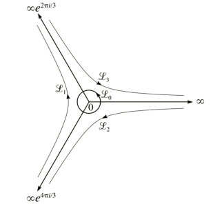 Figure 1
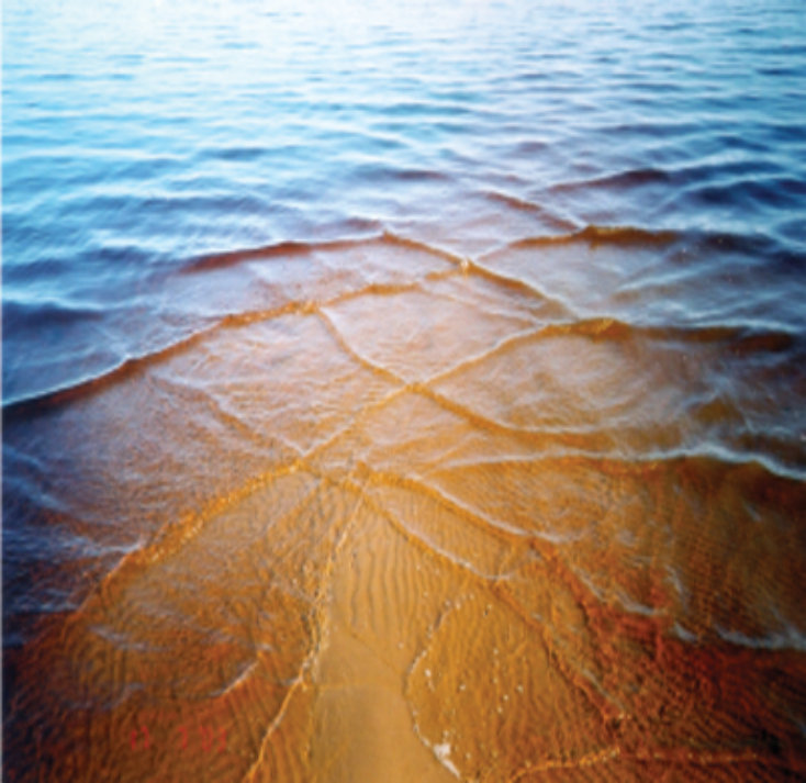 Figure 2
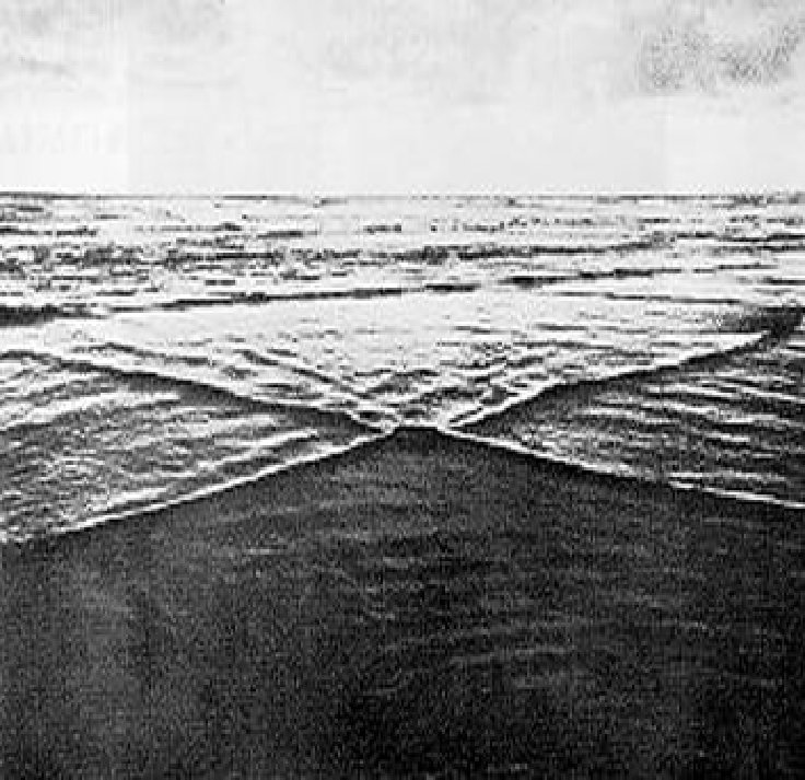 Figure 3
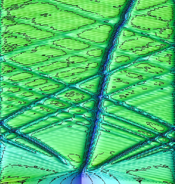 Figure 4
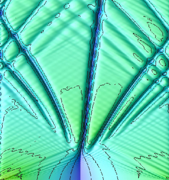 Figure 5
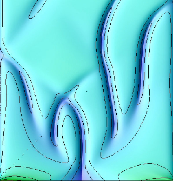 Figure 6
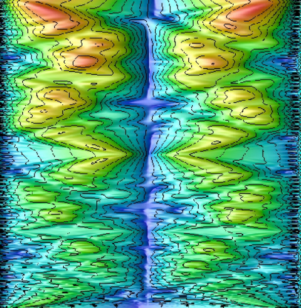 Figure 7
| Profile | ||||
|---|---|---|---|---|
| pCf | ||||
| pPf | ||||
| LBL | ||||
| TBL |
Peer Reviews
No public reviews on file for this paper yet. If you reviewed it on a platform where reviews are public (OpenReview, ICLR, NeurIPS, ICML), you can paste yours below so the community can read it here.
Videos
No videos yet. Explain this paper in a talk, walkthrough, or lecture? Add one.
Taxonomy
TopicsOcean Waves and Remote Sensing · Coastal and Marine Dynamics · Meteorological Phenomena and Simulations
\affiliation
Center for Geophysics and Planetary Physics, Department of Mathematics, Embry-Riddle Aeronautical University, Daytona Beach, FL, U.S.A.
emails: [email protected], [email protected]
Interaction of Tollmien-Schlichting Waves in the Air with the Sea
Surface
Shahrdad G. Sajjadi and Harihar Khanal
Abstract
Tollmien-Schlichting waves, Hydrodynamic stability, Air-sea interaction, Two-fluid interface, Solitons Linear stability of fully developed flows of air over water is carried out in order to study non-linear effects in the generation of solitons by wind. A linear stability analysis of the basic flow is made and the conditions at which solitons first begin to grow is determined. Then, following [10], the non-linear stability of the flow is examined and the quintic non-linear Schrödinger equation is derived for the amplitude of disturbances. The coefficients of the non-linear Schrödinger equation are calculated from the eigenvalue problem which determines the stability of air-water interface.
An asymptotic and a numerical stability analysis is carried out to determine the neutrally stable flow conditions for air-sea interface. Four different profiles are considered for the airflow blowing over the surface of the sea, namely, plane Couette flow (pCf), plane Poiseuille flow (pPf), laminar and turbulent boundary layer (L,TBL) profiles. For each of the above cases the shear flow counterpart in the water is assumed to be a pPf.
A nonlinear stability analysis results in the nonlinear Schrödinger equation
[TABLE]
where and are local variables, and the amplitude of the surface wave is proportional to . The complex constants , , and are evaluated from the linear stability of the two-fluid interface. The profile for the initial condition considered here is that of the Stokes wave
[TABLE]
where is the amplitude and is the wavenumber of the surface Stokes wave.
It is shown that the above amplitude equation produces ‘snake’ solitons [9] for pCf, pPf and LBL profiles, with striking similarities. On the other hand, for TBL we observe a very violent surface motion. For cases of pCf and LBL remarkable similarity is observed with observations made at sea.
We conclude that the effect of nonlinearity in the airflow over the sea surface is much larger than nonlinear interactions in the water, and hence it is not possible to decouple the motion in the air and the water for finite amplitude wind-wave interactions, particularly in the case of wind-generated solitons in shallow waters.
1 Introduction
The wind-generated solitons which moves nondispersively on the thin wind-driven drift layer of wind-excited surface wave waves are important because they are products of the processes under which surface waves are generated by wind. When the local atmospheric conditions are such that significant bubble densities are created, principally by breaking waves, the resulting bubble layer will dominate and mask these solitons, in underwater acoustic scattering. A qualitative mixed linear-nonlinear model of ocean-wave generation is briefly described, a key element of which is the generation of solitons by wind. These solitons are created, and destroyed on moving gravity waves, caused by waves being generated by wind along with accompanying capillary components. The gravity-capillary waves are dispersive, in contrast the solitons are nondispersive, that is to say, they move at constant speed, on the thin moving wind drift layer generated by the upper part of the water surface.
In this paper, we will examine the stability of laminar and turbulent flows of air over water surface where viscous effects are taken into account in both fluids. The flow that will be studied here is the fully developed flow of air over water. In contrast to [2], we shall restrict our analysis to only the case when the motion is driven solely by a constant pressure gradient.
A linear stability analysis will be performed to determine the neutrally stable flow conditions. This approach is different to [4], or indeed other similar theories such as [1], and most experimental work, where the emphasis is on determining wave growth rates rather than the conditions at which waves will first start to grow. Following [10], a non-linear analysis will be performed which will yield the non-linear quintic Schrödinger equation
[TABLE]
governing the wave amplitude. In equation (1) is proportional to amplitude of the non-linear surface wave. The scaled length and time, and , and the complex constants and and will be defined in the proceeding analysis. The constants and are properties of the flow which is obtained from the linear stability theory, while the effect of non-linear interactions is determined by and .
It is to be noted that although equation (1) is strictly applicable to velocity profiles of laminar flow, there are experimental and theoretical suggestions that equations similar to that of (1) are also applicable to wind-wave generation situations. For example, the experimental work [6] suggests that wind-waves at fixed fetch and under steady wind conditions have properties that are similar to non-linear Stokes wavetrains. Indeed, the wind-waves given by the equilibrium amplitude solutions of (1) (for which and ) are similar to Stokes wavetrains
[TABLE]
where is the critical wavenumber, and are the dimensionless energy transfer parameters [13], and is the wave phase speed. It has been shown [11] that such wavetrains with non-linear effects lead to changes in the phase speed of the wave and provides the sideband instability mechanism, similar to that of Benjamin-Fier, which will eventually result to the break-up of the wave-train.
The wind-generated solitons which moves nondispersively on the thin wind-driven drift layer of wind-excited surface wave waves are important because they are products of the processes under which surface waves are generated by wind. When the local atmospheric conditions are such that significant bubble densities are created, principally by breaking waves, the resulting bubble layer will dominate and mask these solitons, in underwater acoustic scattering. A qualitative mixed linear-nonlinear model of ocean-wave generation is briefly described, a key element of which is the generation of solitons by wind. These solitons are created, and destroyed on moving gravity waves, caused by waves being generated by wind along with accompanying capillary components. The gravity-capillary waves are dispersive, in contrast the solitons are nondispersive, that is to say, they move at constant speed, on the thin moving wind drift layer generated by the upper part of the water surface.
In this paper, we will examine the stability of laminar and turbulent flows of air over water surface where viscous effects are taken into account in both fluids. The flow that will be studied here is the fully developed flow of air over water. In contrast to [2], we shall restrict our analysis to only the case when the motion is driven solely by a constant pressure gradient.
2 Formulation of the problem
We consider the steady, flow of two super-imposed fluid layers confined between a stationary horizontal parallel plate, placed at , and open to atmosphere above at a distance . We assume the flow of the upper fluid is turbulent, satisfying Prandtl’s mixing-length model, and that of the lower one is a fully developed laminar flow. The velocity vector \mbox{\boldmathU}=[U_{b}(y),0,0], for the upper fluid, and \mbox{\boldmathu}=[u_{b}(y),0,0], for the lower fluid,111Hereafter, the upper and the lower symbols (Greek or Roman) denote the upper (air) and the lower (water) fluids, respectively. Also the subscripts and denote air and water, respectively. both satisfy the Navier-Stokes equations. In the present case we shall confine ourselves to the case when the motion of the lower fluid is driven solely by a constant pressure gradient. Thus, the equations of motion and their corresponding boundary conditions reduce to
[TABLE]
where The solutions of (8) are given by
[TABLE]
where
[TABLE]
is the friction velocity of the upper fluid, is the von Kármán’s constant, and is an effective roughness length.
Having obtained the velocity fields governing the basic flow, we shall now formulate the non-dimensional equations that govern linear instability. The motion is governed by the three-dimensional Navier-Stokes equations in each layer of fluid. The boundary conditions are the no-slip conditions on the plates and continuity of stress and velocity across the unknown interface , which will be determined from the proceeding non-linear analysis.
We will introduce the following curvilinear coordinates [5]
[TABLE]
where in (17), the minus sign is for the upper media and the plus sign for the lower media. The Jacobian of the transformation is
[TABLE]
Note that, in the linear stability theory we shall be restricted to infinitesimal disturbances for which the Jacobian (18) reduce to
[TABLE]
Thus, within this order of approximation, the governing equations are symbolically the same as that of Cartesian coordinates. We remark that under the transformation (17), the lines and will map to lines and , respectively, and the unknown interface will then be at .
The boundary conditions are:
on no-slip conditions ,
on (the unknown interface);
(i) the continuty of velocities \hskip 25.6073pt\mbox{\boldmathu}=\mbox{\boldmathU}
(ii) the kinematic conditions
[TABLE]
(iii) the continuity of tangential stresses
[TABLE]
(iv) the dynamic condition
[TABLE]
where , and Also, on there is no-slip conditions .
In (29) is the Reynolds number, is the Froude number and is the Weber number, where is a reference velocity, is the dimensional surface tension and is the acceleration due to gravity.
We next perturb the basic flow by infinitesimal disturbances, i.e.
[TABLE]
where c.c. denotes a complex conjugate, then the linearized equations of motion may be cast as
[TABLE]
Substituting in equations of motion and their corresponding boundary conditions, making use of the Squire transformation [14] , etc. (dropping the hat notation) and introducing the stream functions and such that
[TABLE]
we obtain, after linearization and some manipulations,
[TABLE]
where . Note that, we have redefined the Froude and Weber number to be and , respectively.
Systems similar to that of (84) have been derived [7,15–17]. However, as was pointed out by Blennerhassett [2], in the derivations [7,17] the relevance of and to the stability of two-dimensional waves was not noted. He further remarks that in earlier derivations [15,16], for the stability of superposed fluid layers, the terms and was incorrectly omitted from the second interface condition in the system (84).
We remark that in general the solution of (84), and determining the location of the neutral stability curve in –plane is a computational task. The full details of the numerical methods is given in section 6 below.
3 The long-wave limit
Following [2], we consider the stability of the basic flow in the limit of long wavelength disturbances and expand the eigenfunctions and the eigenvalue in regular perturbation series in [7]. Thus we may write
[TABLE]
as for a fix value of . Substituting (90) in (84) we obtain up to the following homogeneous system
[TABLE]
In the case of pPf, the system (109) has a eigensolution
[TABLE]
and
[TABLE]
The eigenvalue is given by
[TABLE]
Similarly, in the limit of slow basic flow, when the Reynolds number for the basic flow is small, we may expand , and as for fixed and . Thus we obtain a system similar to (109) whose solution is
[TABLE]
where and , and the eigenvalues and the constants and are determined by applying the interface conditions at . This yields a homogeneous set of equations whose non-trivial solutions can only be obtained for certain values of .
We next consider . To this order the system (84) reduce to
[TABLE]
Since and are real, we can easily see that is purely imaginary. Note that the homogeneous part (134) is the same as (109). Thus, in order that the inhomogeneous system to have a solution we must satisfy certain solvability criterion. We introduce the adjoint functions [6], and , and write down the system which is adjoint to (134)
[TABLE]
with the adjoint condition 222Stuart’s solvability criterion states that if is a differential operator and is its adjoint operator, then if and its adjoint is given by the solvability condition states
which implies
[TABLE]
The eigenvalue for the adjoint system (148) is the same as that of (109), while the adjoint functions for pPf are
[TABLE]
When the solvability condition is applied to (109) we obtain the following expression for :
[TABLE]
To , the condition for neutral stability is that . Hence, from (149) we obtain the following relationship between and :
[TABLE]
Equation (150) is a quadratic in which may be expressed as
[TABLE]
with its solutions given by
[TABLE]
Since , we obtain the following compact relation between the wavenumber and the Reynolds number , i.e.
[TABLE]
4 The short-wave limit
We shall now focus our attention to conditions under which short-wavelengths disturbances may grow along the interface. We shall pose the following restrictions on the problem
[TABLE]
To study this, we will adopt an asymptotic analysis for pPf. However, before we commence with our analysis, it is convenient to express the interfacial boundary conditions (84) in more compact mathematical form. We do this by defining
[TABLE]
Thus, the second to the fourth interfacial conditions (84) may be written as
[TABLE]
We shall also scale the coordinates with the wavenumber such that
[TABLE]
and assume the following asymptotic expansions for and :
[TABLE]
Neglecting terms of by invoking the restriction (a) in (24), replacing the independent variable by and defining , the eigenfunction for the lower fluid will satisfy the following Orr-Sommerfeld equation
[TABLE]
in which we anticipate .
Since the effective Reynolds number, , is large, we may neglect the viscous terms in (177) and thus reduce it to the Rayleigh equation
[TABLE]
Equation (178) has a regular solution
[TABLE]
and a solution with logarithmic branch point at and , namely
[TABLE]
where the superscript in (179) and (180) denotes the outer solution.
Now to recover the boundary layer near the interface, and following the usual practice in the theory of hydrodynamic stability, we introduce and let . Thus, (177) becomes
[TABLE]
Expanding in powers of we obtain, at zero order in
[TABLE]
and at we get
[TABLE]
The solution of (182) is
[TABLE]
In (184), , denote generalized Airy function
[TABLE]
where is the appropriate path of integrals shown in figure 1.
For the generalized Airy function is exponentially large. Thus we set the constant in (184). The constants and are found by matching (184) with the inviscid solutions (179) and (180). However, to do this we require the next-order solutions to the constant and linear parts in (184).
From (184) we see that
[TABLE]
where the superscript represent the inner solution and is a generalized Airy function given by
[TABLE]
Now matching with , and with , we obtain, respectively
[TABLE]
where is the psi function.
To evaluate the above integral we note that
[TABLE]
where Ai is the usual Airy function. Using the asymptotic representation of the generalized Airy function
[TABLE]
and the following relationship
[TABLE]
it can be shown that
[TABLE]
Note that, solutions of this kind are used as an initial guess for the full numerical integration.
5 Nonlinear stability
The governing equations and boundary conditions for the two-dimensional motion of two superposed fluids in curvilinear coordinates are
[TABLE]
where the upper and lower case symbols refer to fluids above and below the interface, respectively, and ; ; and , being the ratio of the height above and below the interface. Here, , , and are dimensionless density, dynamic viscosity and kinematic viscosity, respectively, with understanding that the suffices and refer to air and water. Also, , and are the Froude, Weber and Reynolds numbers respectively, with denoting the acceleration due to gravity, the coefficient of surface tension, the free stream speed of the air, and is the interface profile which is the Stokes wave.
For the disturbance near theocratical conditions we expand the frequency and eigenfunction as a Taylor series. Thus
[TABLE]
Now, since , then is the group velocity of the disturbance; is related to the curvature of the nose of the neutral curve and is the exponential growth of the wave for . Likewise we expand in the form
[TABLE]
with a similar expansion for in the lower fluid.
It is well known that the basic flow becomes unstable to travelling wave disturbances when [3,8]. To examine the growth of these Tollmien-Schlichting waves in the vicinity of we introduce the small parameter
[TABLE]
and scaled variable
[TABLE]
The continuity equations in (222) are satisfied by the streamfunctions and for the upper and lower fluids, respectively, thus
[TABLE]
Introducing the expansions
[TABLE]
where c.c. denotes complex conjugate, and We further expand the functions in (227) as
[TABLE]
The pressure and interface displacement are expanded as
[TABLE]
where
[TABLE]
Substituting in (222) and equating powers of we obtain the coupled Orr-Sommerfeld problem
[TABLE]
Note that the system (254) is the same as (84) with , and . The solution of (254) may be written as
[TABLE]
where is the amplitude function to be determined.
The distortion of the mean flow occurs at , which is
[TABLE]
where
[TABLE]
and a tilde denotes complex conjugate. The system (254) has unique solution of the form
[TABLE]
where
[TABLE]
The constants and are found by applying the interface conditions.
At we obtain the system governing the second harmonic, namely
[TABLE]
The solution of (325) may be expressed as
[TABLE]
with the assumption that the solution is unique.
We emphasize that the adjoint equation in the upper and he lower fluid layer is the adjoint of the Orr-Sommerfeld equation for a homogeneous fluid. The adjoint system possesses the following relationship
[TABLE]
where the operators and are the same as that given in (254), and
[TABLE]
The system of equations for is given by
[TABLE]
where UF and LF stands for upper and lower fluid, respectively. The solution of the system is
[TABLE]
where is and arbitrary function of and , and and are the solutions of the following system
[TABLE]
since the adjoint to the system (84), at critical conditions, satisfies
[TABLE]
Next, at , we obtain the system of equations
[TABLE]
where
[TABLE]
Proceeding as above we obtain the following set of equations at .
[TABLE]
where
[TABLE]
and
[TABLE]
In (425), the remaining coefficients are given by Blennerhassett [2].
This system of equations has a unique solution provided the inhomogeneous terms are orthogonal to the adjoint function. Applying the solvability condition yields the amplitude equation (1).
The complex coefficients , and in equation (1) are given by
[TABLE]
where satisfies the Orr-Sommerfeld equation for the basic flow with satisfying their adjoints.
It is important to note that in the formulation presented here quantities such as and , and their adjoints, are functions of alone, but, by virtue of (17) they are functions of both spacial coordinates , and time . Also, since the Jacobian of the transformation is , the resulting equations expressed in curvilinear coordinates are, to first order in , symbollically identical to their Caretesian counterpart. Thus, the solutions for the basic flow, in curvilinear coordinates, are the same as those given by (10) and (489), in Cartesian coordinates, with simply replaced with . The error in this approximation is and may be neglected since .
6 Numerical Schemes
The complex cubic–quintic nonlinear Schrödinger equation (1) is solved numerically, using a second-order central difference for the spacial part and the third-order explicit Runge-Kutta method for the transient part, whose complex coefficients are determined from the system of ordinary differential equations (254), (329) and (329) which coupled via interface conditions which are solved numerically using the finite difference scheme as described below. First, we rewrite the system in a compact form as
[TABLE]
where , and the definitions of the coefficients , , , , , , , , , , , are those given by system of equation (254), (329) and (395), respectively.
We approximate
[TABLE]
where is the usual central difference operator, i.e., . Then
[TABLE]
Here and is defined as .
For we use the following approximation
[TABLE]
Using (474) and the appropriate equation of motion from (466), we have
[TABLE]
Hence we maintain accuracy and a five point formula for the third derivative in the interface. The similar expressions result for the derivatives of . Substituting (471)–(473) in (466), we obtain the following finite difference approximation.
[TABLE]
where
[TABLE]
where the subscript implies evaluation at . Similar expressions result for the approximation to . Thus, the finite difference approximation to the coupled ODEs system with the boundary conditions and the interface condition (466) leads to the matrix equation with the following form:
[TABLE]
where the entries of the matrix and unknown vector are complex numbers.
6.1 Complex cubic–quintic nonlinear Schrödinger equation
Let be the grid spacing and be the grid points. Define as an approximation to , and . Let . Using the central difference approximation to , we write the semi–discretization of the IBVP for equation (1) as the following system of ODEs
[TABLE]
where . The upper dot in (481) indicates derivative with respect to and is the finite difference matrix.
To construct an integration scheme to solve the ODE system (481)–(482), let , and let denote the value of the variable at time . Employing a low storage variant third–order Runge–Kutta scheme [12], we write the fully discrete system as
[TABLE]
where .
The numerical scheme is parallelized for distributed memory clusters of processors or heterogeneous networked computers using the MPI (Message Passing Interface) library and implemented in FORTRAN.
7 Results
For the numerical simulation reported in this paper, we choose and for the present case of wind blowing over waves. Here the quantity is defined as
[TABLE]
with , , , , and we choose such that . The kinematic viscosities are taken to be and .
The velocity profiles for the basic flow, for the case of turbulent boundary layer, are those given by (8). The velocity profiles for pPf and pCf, for the upper fluid, satisfy
[TABLE]
The solution of this system is given by [2]
[TABLE]
where
[TABLE]
and
[TABLE]
Note that, for pPf which implies that he upper boundary is stationary, and the flow is driven by the pressure gradient. In contrast, for pCf and the motion is generated soley by the relative motion of the boundaries.
Computations were performed on a Linux cluster (zeus.db.erau.edu: 256 Intel Xeon 3.2GHz 1024 KB cache 4GB with Myrinet MX, GNU Linux) at Embry-Riddle University. In all simulations presented here, we use the spacial domain of and temporal domain , the typical values of the parameters , for the amplitude and the wavelength of the Stokes wave profile, respectively, and the other parameters of the model (1) are given in Table 1 below.
Figure 2 shows the surface structure for pCf (left) and pPf (right). For the case of pPf we observe the classical ‘snake’ type solitons [9], whereas for pCf we see a different structure similar to colliding solitons which, in time, bifurcates to weaker soliton structure.
In figure 3 the surface structure for LBL (left) and TBL (right) are depicted. As can be seen, the soliton structures for TBL resembles the chaotic solitons [9]. This is, of course, not surprising as turbulence generates more complex surface agitation compared to its laminar counterpart. We may term this as a violent surface motion.
The most intriguing results obtained is that shown in figure 3 for LBL. This results clearly confirms the generation of solitons by wind, which has commonly been observed is shallow waters, c.f. figure 4.
8 Conclusions
In this paper we presented an asymptotic theory for linear stability of non-linear air-sea interfaces by taking into account the motion in the air and the water. The two motions are then matched at the free surface via the usual kinematic, dynamic and free stress boundary conditions. The flow above water is assumed to be turbulent, with a mean logarithmic velocity profile. On the other hand, a plane Poiseuille flow is assumed for the motion in the water. Also presented, is the linear stability calculations of two fluid interface which suggest the flow become unstable for wavenumbers above that given by equation (23). Finally, the growth of surface waves by the shear wind blowing over is calculated. It is shown and extra term arises in the expression for the dimensionless energy transfer parameter which is due to the coupling between wind and surface waves.
In the second part of this paper [3], we use a non-linear hydrodynamic stability [7] to derive the quintic non-linear Schrödinger equation (1) with complex coefficients. We then use the above analysis to determine the complex amplitude of the equation (1).
Using a nonlinear stability analysis of a coupled air-sea system is performed. An amplitude equation, namely the quintic nonlinear Schrödinger equation with complex coefficients is derived. The complex coefficients are obtained from the linear stability of the same system in the neighborhood of the critical Reynolds number. Four different profiles for the shear flow for the airflow over the interface is considered, namely, plane Couette flow (pCf), plane Poiseuille flow (pPf), laminar and turbulent boundary layer (L,TBL) profiles. For each of the above cases the shear flow counterpart in the water is assumed to be a pPf.
It is shown that the above amplitude equation produces ‘snake’ solitons for pCf, pPf and LBL profiles, with striking similarities. On the other hand, for TBL we observe a very violent surface motion. For cases of pCf and LBL remarkable similarity is observed with observations made at sea.
We conclude that the effect of nonlinearity in the airflow over the sea surface is much larger than nonlinear interactions in the water, and hence it is not possible to decouple the motion in the air and the water for finite amplitude wind-wave interactions. We remark, under the conditions shown in this paper, the generation of solitons by wind is possible particularly in shallow waters.
The reference list from the paper itself. Each links out to its DOI / PubMed record.
- 1(1)
- 2(2) [1] S.E. Belcher and J.C.R. Hunt , Turbulent shear flow over slowly moving waves. J. Fluid Mech. , 251 , 109–148. 1993.
- 3(3)
- 4(4) [2] P.J. Blennerhassett , On the generation of waves by wind. Phil. Trans. Roy. Soc. , A 298 , 451-494, 1980.
- 5(5)
- 6(6) [3] S. Feldman , On the hydrodynamic stability of two viscous incompressible fluids in parallel uniform shearing motion. J. Fluid Mech. , 2 , 343-370, 1957.
- 7(7)
- 8(8) [4] H. Khanal and S.C. Mancas , Numerical simulations of five novel classes of dissipative solitons. CMMSE Proceedings , Vol II, 354-365, 2008.