Ultra-deep Large Binocular Camera U-band Imaging of the GOODS-North Field: Depth vs. Resolution
Teresa A. Ashcraft, Rogier A. Windhorst, Rolf A. Jansen, Seth H., Cohen, Andrea Grazian, Diego Paris, Adriano Fontana, Emanuele Giallongo,, Roberto Speziali, Vincenzo Testa, Konstantina Boutsia, Robert W. O'Connell,, Michael Rutkowski, Russell Ryan, Claudia Scarlata

TL;DR
This study compares the effects of image resolution and depth in U-band observations of the GOODS-North field, revealing how resolution impacts object detection, galaxy structure visibility, and flux measurements at faint magnitudes.
Contribution
It provides a detailed analysis of the trade-off between image depth and resolution in deep field imaging, highlighting the benefits of deeper, lower-resolution mosaics for faint object detection.
Findings
Optimal resolution images detect fewer faint objects beyond U_AB=27 mag.
Deeper images reveal more galaxy structure and clumpy features.
Flux measurements are consistent within 0.5 mag for most bright galaxies.
Abstract
We present a study of the trade-off between depth and resolution using a large number of U-band imaging observations in the GOODS-North field (Giavalisco et al. 2004) from the Large Binocular Camera (LBC) on the Large Binocular Telescope (LBT). Having acquired over 30 hours of data (315 images with 5-6 mins exposures), we generated multiple image mosaics, starting with the best atmospheric seeing images (FWHM 0.8"), which constitute 10% of the total data set. For subsequent mosaics, we added in data with larger seeing values until the final, deepest mosaic included all images with FWHM 1.8" (94% of the total data set). From the mosaics, we made object catalogs to compare the optimal-resolution, yet shallower image to the lower-resolution but deeper image. We show that the number counts for both images are 90% complete to .…
Click any figure to enlarge with its caption.
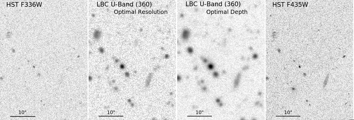 Figure 1
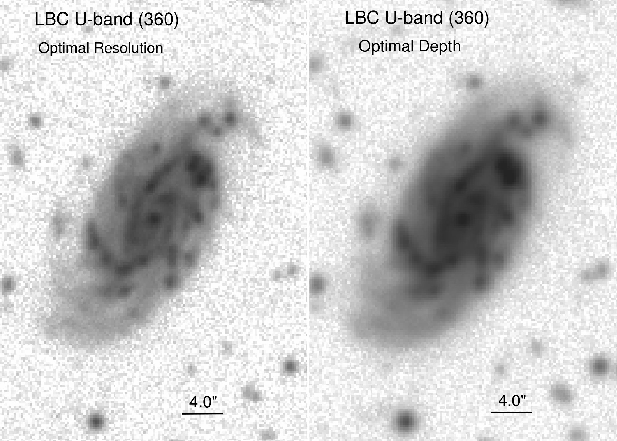 Figure 2
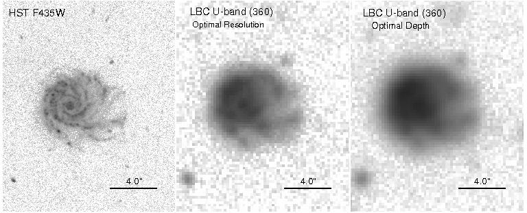 Figure 2
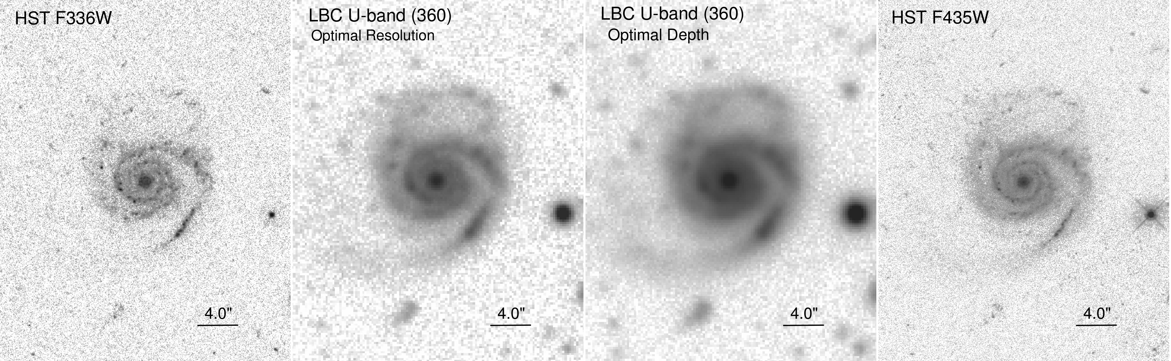 Figure 2
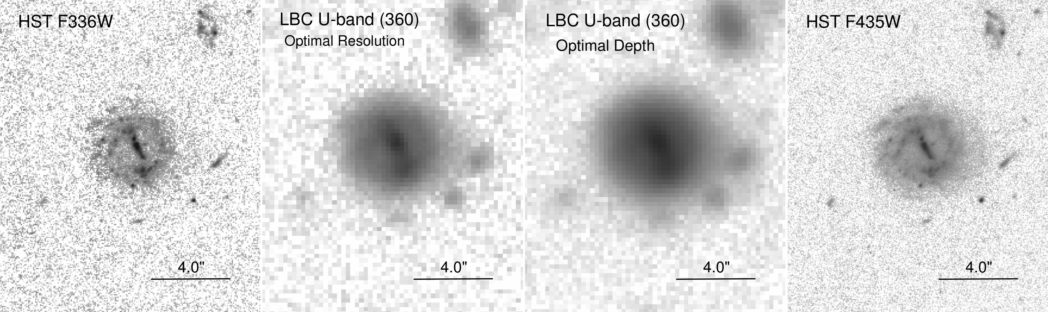 Figure 2
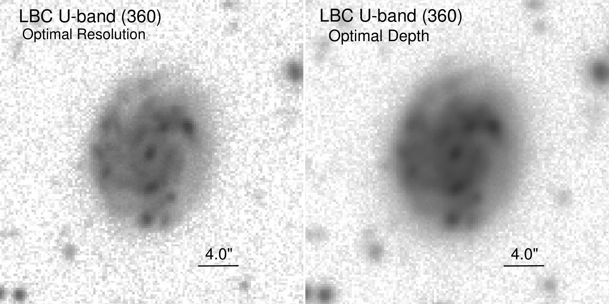 Figure 2
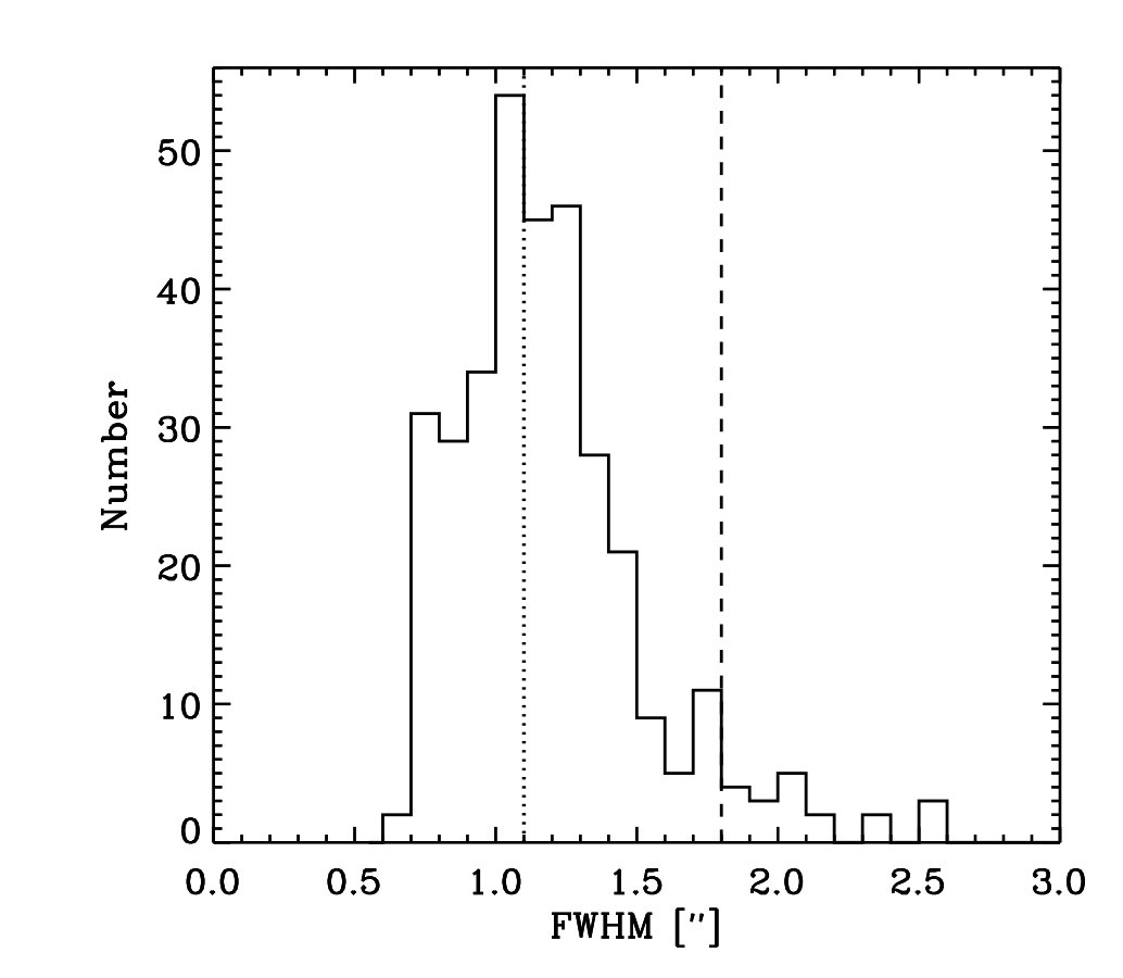 Figure 7
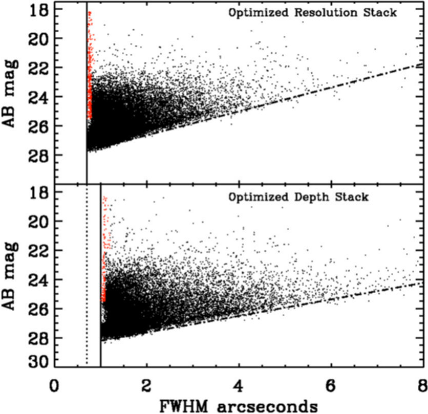 Figure 8
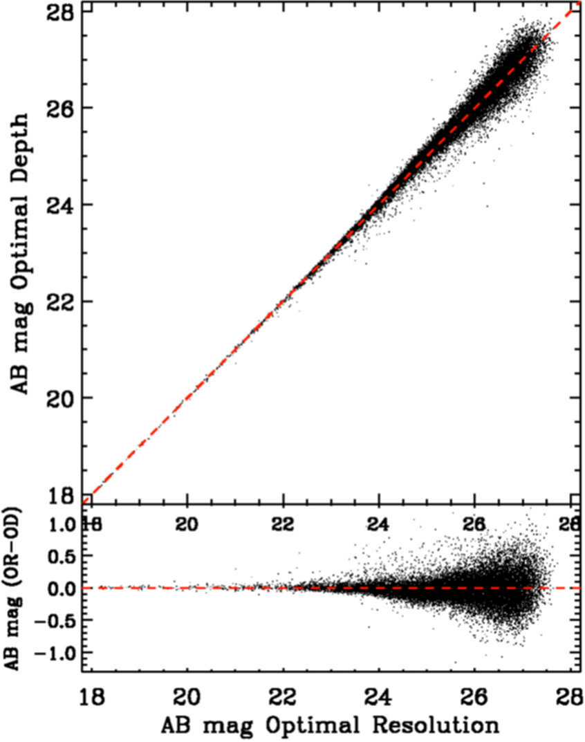 Figure 9
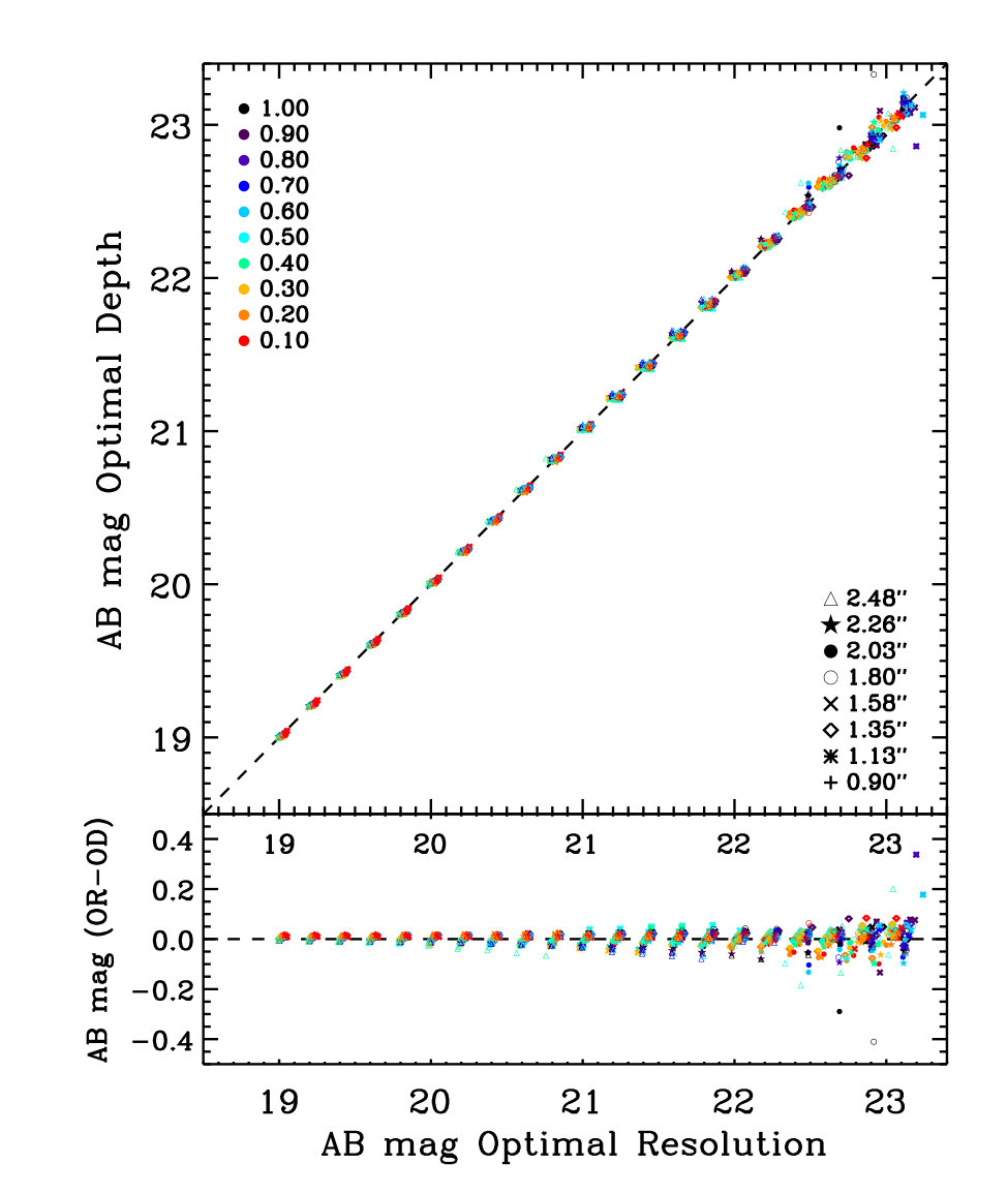 Figure 10
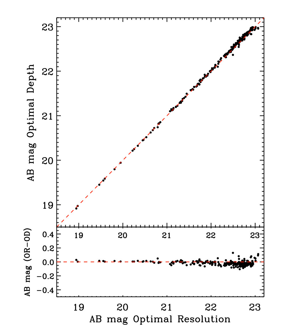 Figure 11
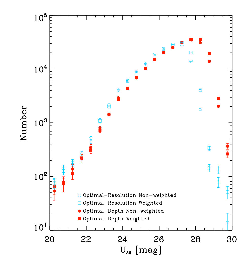 Figure 12
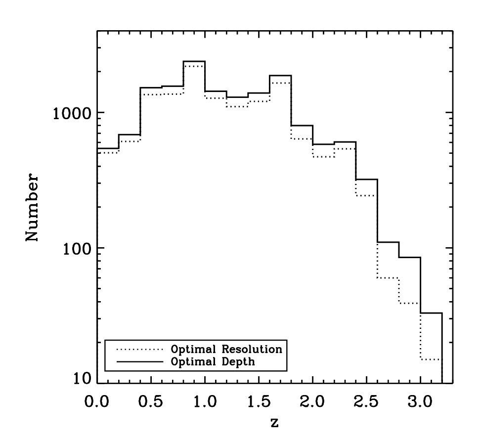 Figure 13
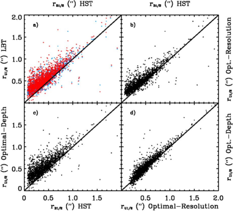 Figure 14
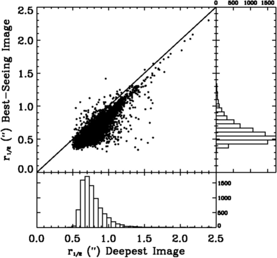 Figure 15
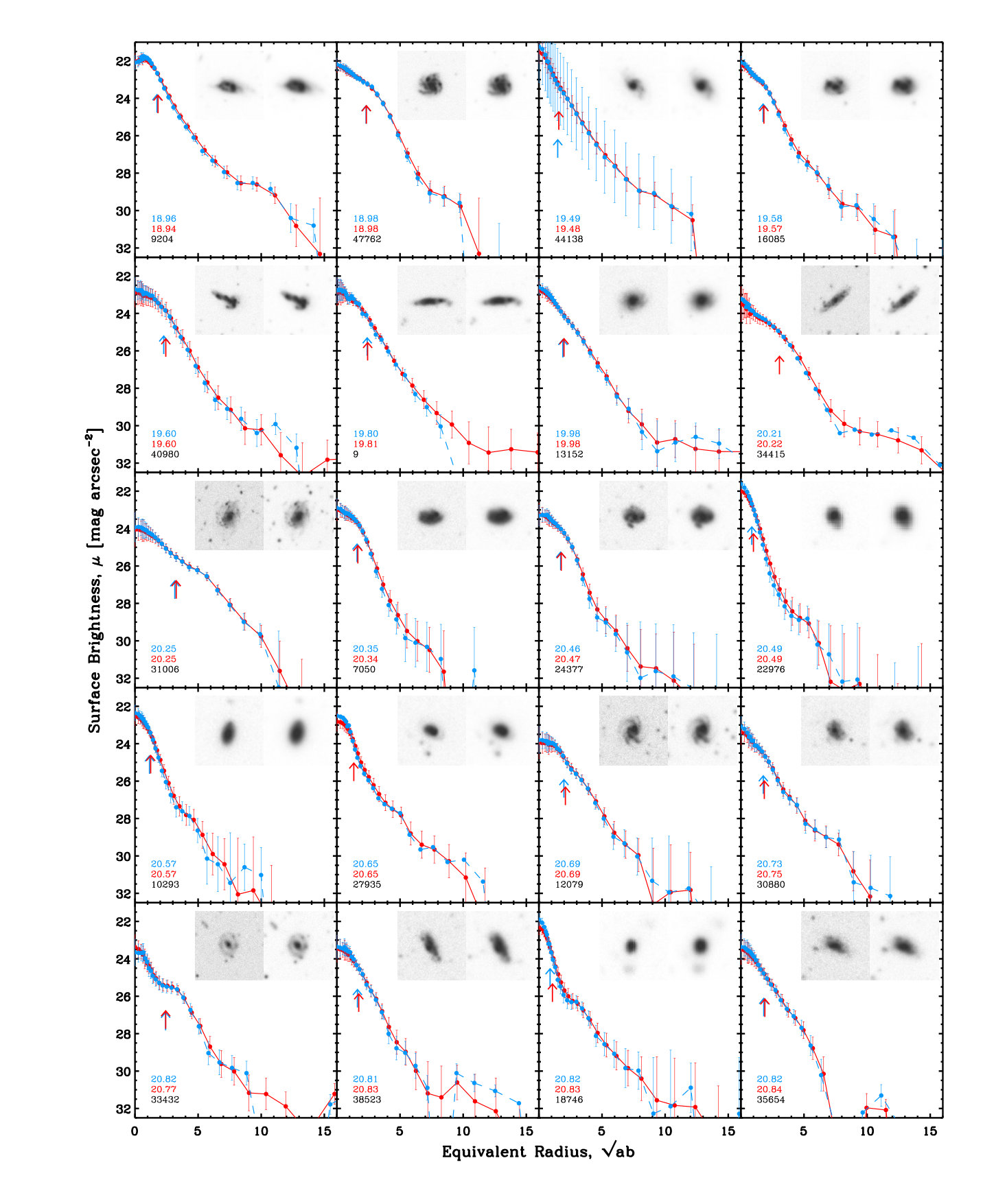 Figure 16
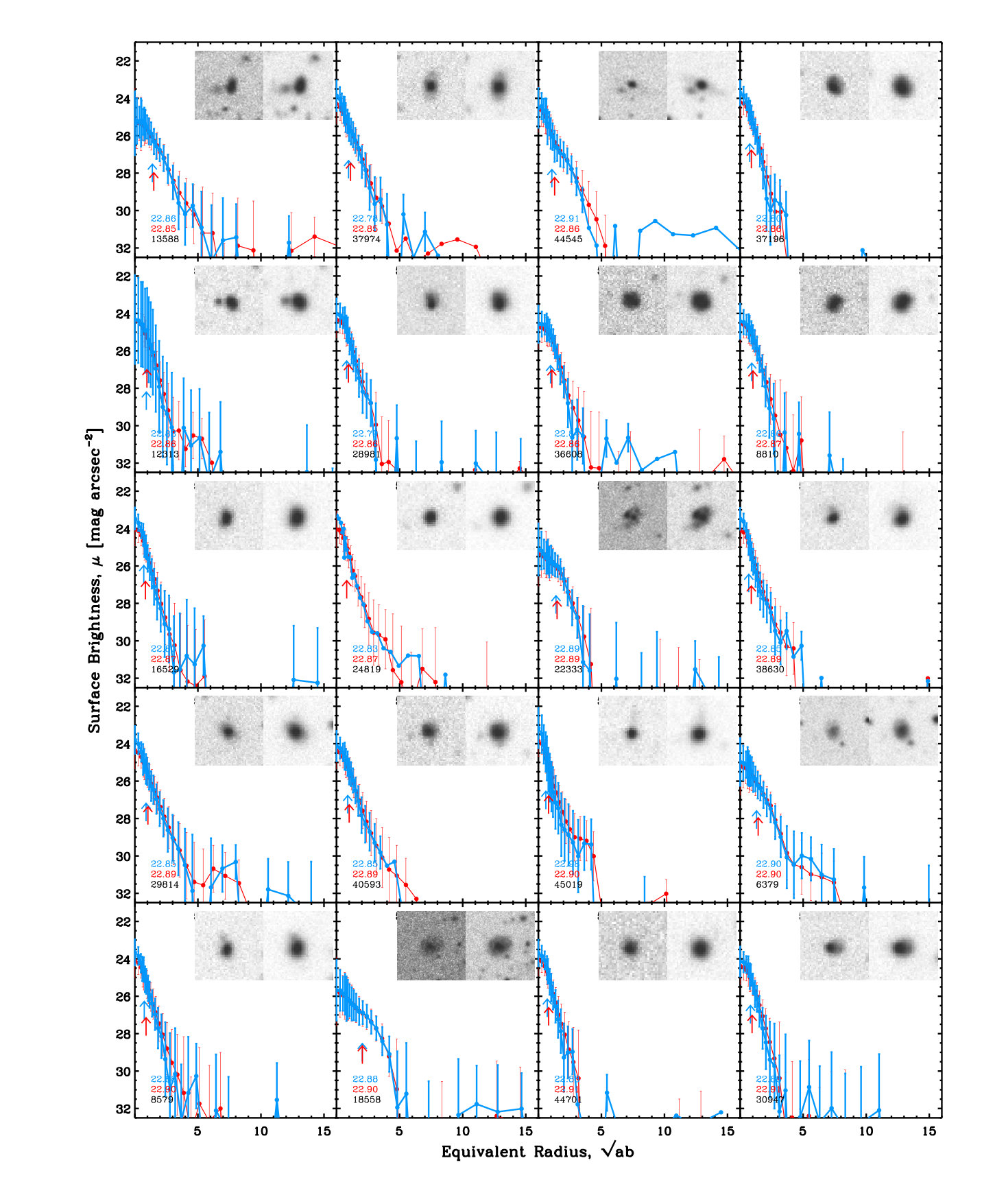 Figure 17
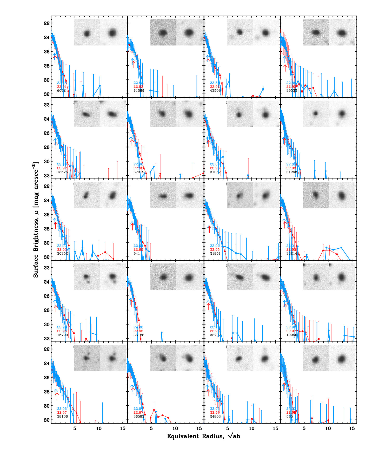 Figure 18
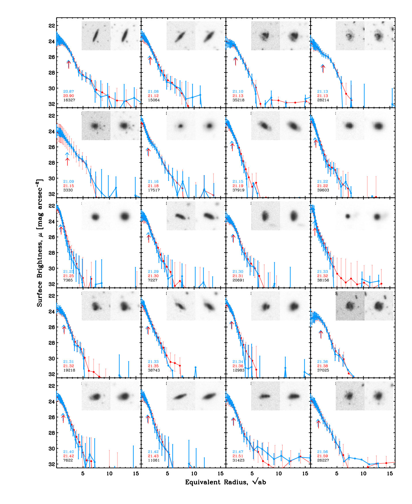 Figure 19
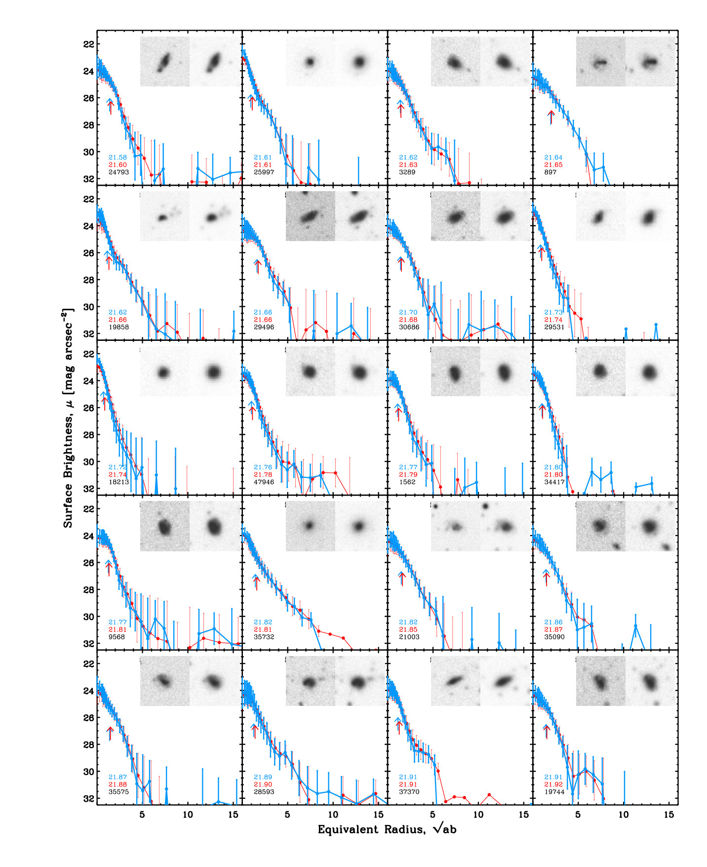 Figure 20
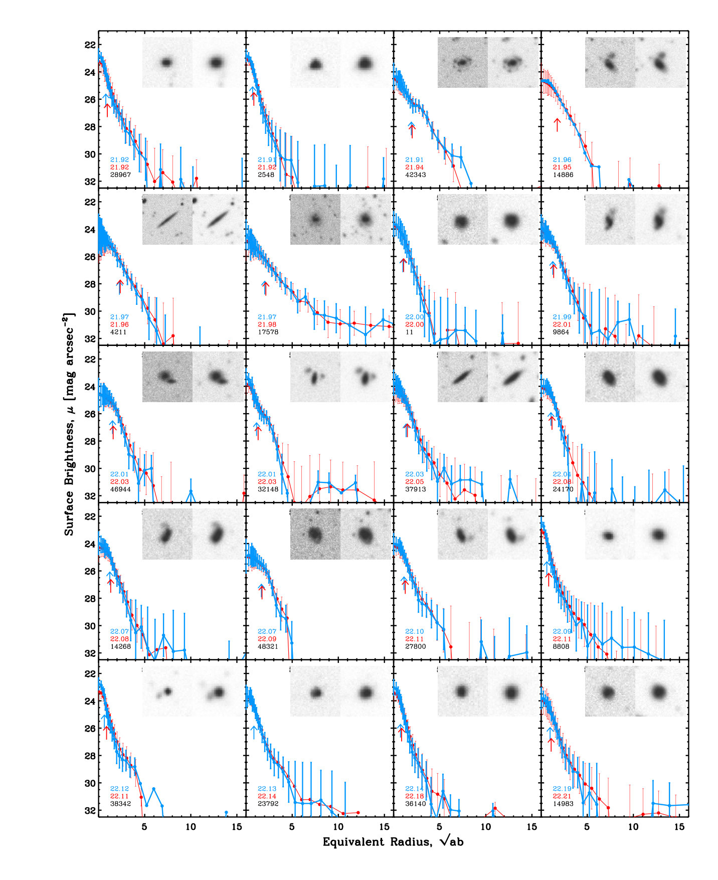 Figure 21
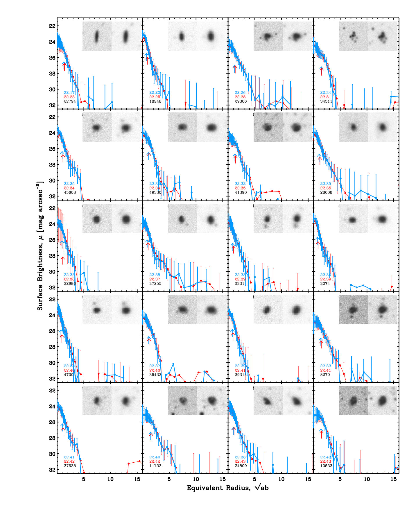 Figure 22
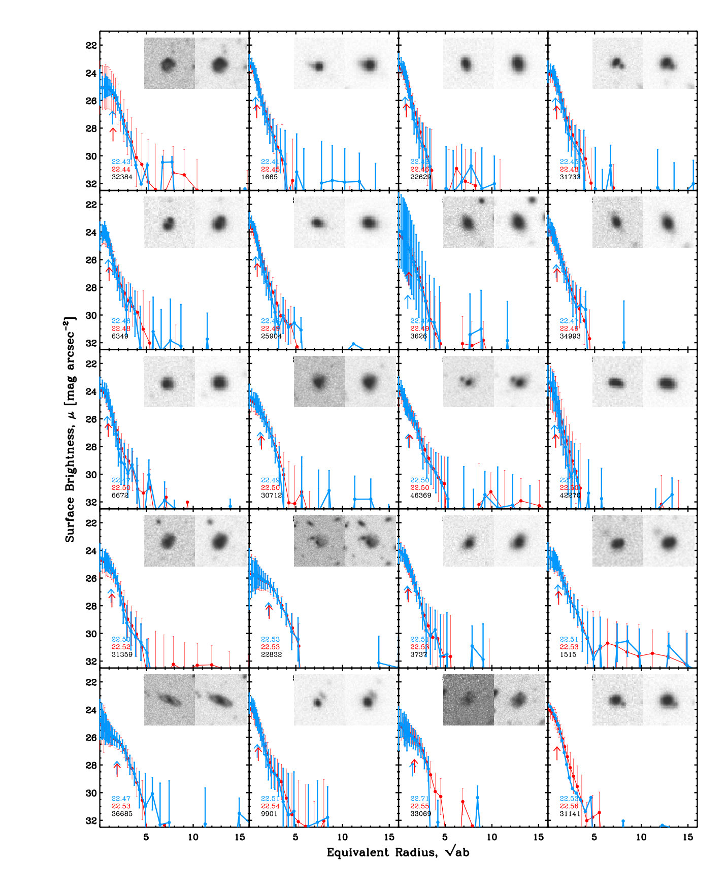 Figure 23
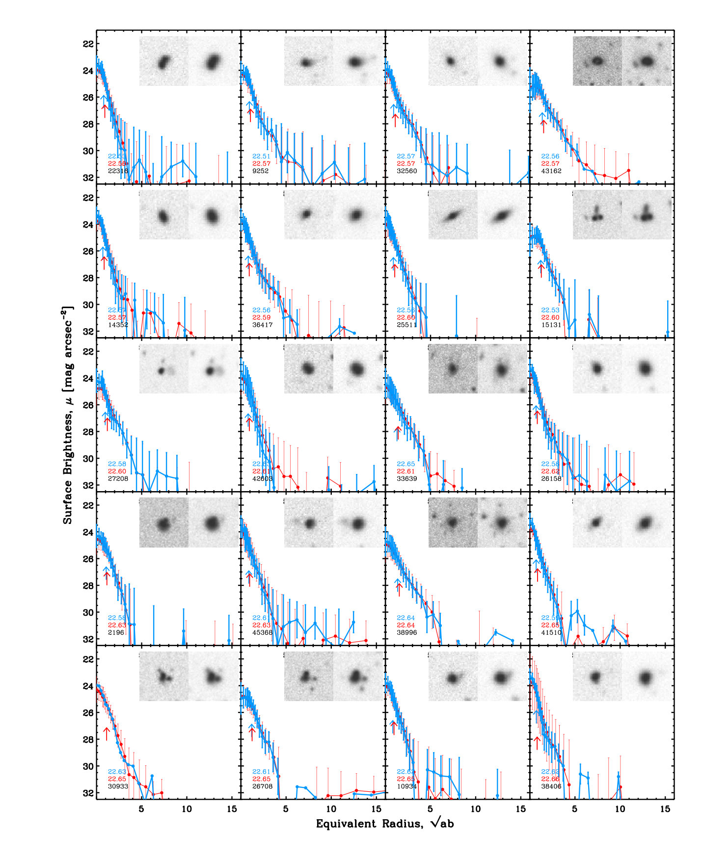 Figure 24
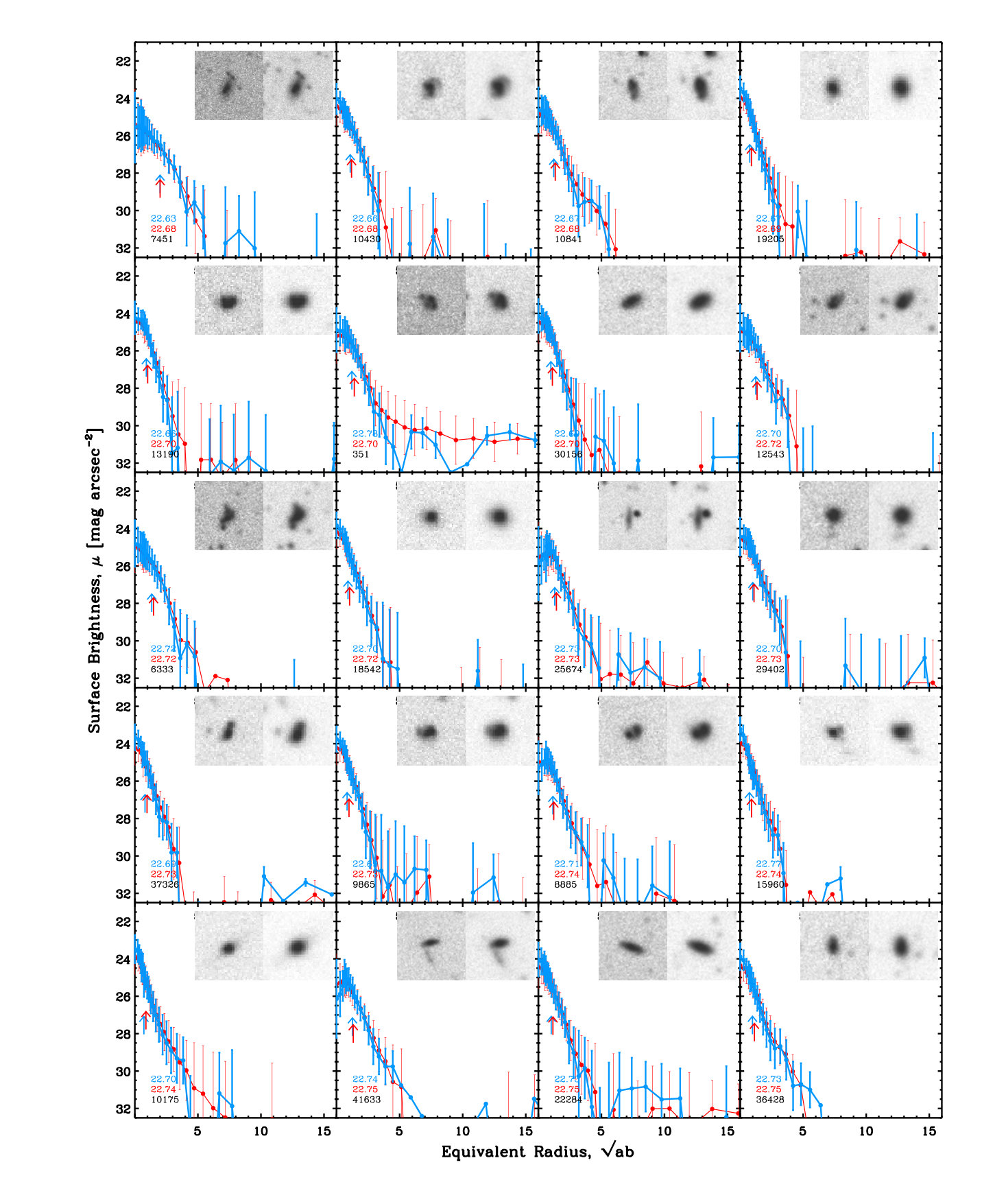 Figure 25
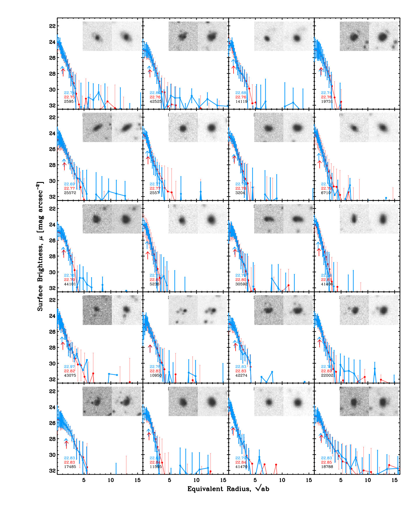 Figure 26
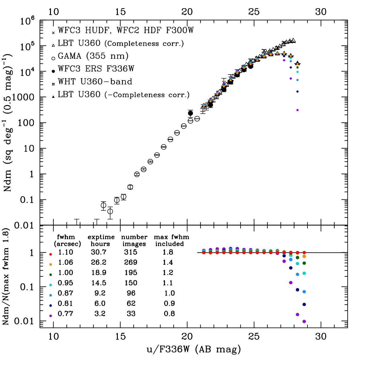 Figure 27
| Group | Number of | Exposure Time | Total Exposure |
|---|---|---|---|
| Images | Per Image (s) | Time (Hours) | |
| Italian | 272 | 360 | 27.22 |
| US | 75 | 300 | 6.25 |
| Keyword | Value |
|---|---|
| COMBINE_TYPE | Median |
| WEIGHT_TYPE | MAP_WEIGHT |
| PIXELSCALE_TYPE | Median |
| CENTER (J2000) | 12:36:54.5, +62:15:41.1 |
| IMAGE_SIZE (pix) | 6351, 6751 |
| RESAMPLING_TYPE | LANCZOS3 |
| Keyword | Optimized Resolution | Optimized Depth |
|---|---|---|
| DETECT_MINAREA | 5 | 5 |
| DETECT_THRESH | 1.0 | 1.0 |
| ANALYSIS_THRESH | 1.0 | 1.0 |
| DEBLEND_NTHRESH | 64 | 64 |
| DEBLEND_MINCONT | 0.06 | 0.04 |
| WEIGHT_TYPE | MAP_RMS | MAP_RMS |
| Number of | Exposure Time | FWHM | Depth |
|---|---|---|---|
| Stacked Images | (Hours) | (arcsec) | (Mag) |
| 033 | 03.2 | 0.77 | 27.0 |
| 062 | 06.0 | 0.81 | 27.4 |
| 096 | 09.1 | 0.87 | 27.6 |
| 150 | 14.2 | 0.96 | 27.8 |
| 195 | 18.8 | 1.00 | 28.0 |
| 241 | 23.2 | 1.03 | 28.1 |
| 269 | 26.0 | 1.06 | 28.2 |
| 290 | 28.1 | 1.08 | 28.2 |
| 315 | 30.4 | 1.10 | 28.3 |
Peer Reviews
No public reviews on file for this paper yet. If you reviewed it on a platform where reviews are public (OpenReview, ICLR, NeurIPS, ICML), you can paste yours below so the community can read it here.
Videos
No videos yet. Explain this paper in a talk, walkthrough, or lecture? Add one.
Taxonomy
TopicsSeismic Imaging and Inversion Techniques · Adaptive optics and wavefront sensing
Ultra-deep Large Binocular Camera U-band Imaging of the GOODS-North Field: Depth vs. Resolution111Based on data acquired using the Large Binocular Telescope (LBT)
Teresa A. Ashcraft
School of Earth and Space Exploration, Arizona State University, Tempe, AZ 85287-1404, USA
Rogier A. Windhorst
School of Earth and Space Exploration, Arizona State University, Tempe, AZ 85287-1404, USA
Rolf A. Jansen
School of Earth and Space Exploration, Arizona State University, Tempe, AZ 85287-1404, USA
Seth H. Cohen
School of Earth and Space Exploration, Arizona State University, Tempe, AZ 85287-1404, USA
Andrea Grazian
INAF - Osservatorio Astronomico di Roma, via Frascati 33, I-00078 Monte Porzio Catone, Italy
Diego Paris
INAF - Osservatorio Astronomico di Roma, via Frascati 33, I-00078 Monte Porzio Catone, Italy
Adriano Fontana
INAF - Osservatorio Astronomico di Roma, via Frascati 33, I-00078 Monte Porzio Catone, Italy
Emanuele Giallongo
INAF - Osservatorio Astronomico di Roma, via Frascati 33, I-00078 Monte Porzio Catone, Italy
Roberto Speziali
INAF - Osservatorio Astronomico di Roma, via Frascati 33, I-00078 Monte Porzio Catone, Italy
Vincenzo Testa
INAF - Osservatorio Astronomico di Roma, via Frascati 33, I-00078 Monte Porzio Catone, Italy
Konstantina Boutsia
Carnegie Observatories, Las Campanas Observatory, Colina El Pino, Casilla 601, La Serena, Chile
Robert W. O’Connell
Department of Astronomy, University of Virginia, Charlottesville, VA 22904-4325, USA
Michael J. Rutkowski
Stockholm University, Department of Astronomy & Oskar Klein Centre for Cosmoparticle Physics, AlbaNova University Centre, SE-106 91 Stockholm, Sweden
Russell E. Ryan
Space Telescope Science Institute, Baltimore, MD 21218, USA
Claudia Scarlata
Minnesota Institute for Astrophysics, University of Minnesota, 116 Church Street SE, Minneapolis, MN 55455, USA
Benjamin Weiner
Steward Observatory, 933 N. Cherry St., University of Arizona, Tucson, AZ 85721, USA
Abstract
We present a study of the trade-off between depth and resolution using a large number of U-band imaging observations in the GOODS-North field (Giavalisco et al. 2004) from the Large Binocular Camera (LBC) on the Large Binocular Telescope (LBT). Having acquired over 30 hours of data (315 images with 5-6 mins exposures), we generated multiple image mosaics, starting with the best atmospheric seeing images (FWHM ), which constitute 10% of the total data set. For subsequent mosaics, we added in data with larger seeing values until the final, deepest mosaic included all images with FWHM (94% of the total data set). From the mosaics, we made object catalogs to compare the optimal-resolution, yet shallower image to the lower-resolution but deeper image. We show that the number counts for both images are 90% complete to . Fainter than 27, the object counts from the optimal-resolution image start to drop-off dramatically (90% between = 27 and 28 mag), while the deepest image with better surface-brightness sensitivity ( 32 mag arcsec*-2*) show a more gradual drop (10% between 27 and 28 mag).
For the brightest galaxies within the GOODS-N field, structure and clumpy features within the galaxies are more prominent in the optimal-resolution image compared to the deeper mosaics. To further investigate how the seeing conditions affect the mosaics, we combined the images by weighting based on the image FWHM. In these weighted stacks, a larger number of small faint galaxies are detected. We conclude that for studies of brighter galaxies and features within them, the optimal-resolution image should be used. However, to fully explore and understand the faintest objects, the deeper imaging with lower resolution are also required. Finally, we find — for 220 brighter galaxies with 24 mag — only marginal differences in total flux between the optimal-resolution and lower-resolution light-profiles to 32 mag arcsec*-2*. In only 10% of the cases are the total-flux differences larger than 0.5 mag. This helps constrain how much flux can be missed from galaxy outskirts, which is important for studies of the Extragalactic Background Light.
techniques: image processing - methods: data analysis - filters: U-band - telescopes: seeing - galaxies: Extragalactic Background Light
††journal: Submitted to PASP; Open to comments from the community
1 INTRODUCTION
In the past 15 years of operation of the Hubble and Chandra space telescopes, a handful of regions of the sky have been studied to probe the distant universe over relatively wide fields with the aim of understanding the assembly of faint galaxies (e.g., the Cosmic Assembly Near-infrared Deep Extragalactic Legacy Survey, “CANDELS”: Cosmic Evolution Survey, “COSMOS”; UKIDSS Ultra-Deep Survey, “UDS”; Extended Groth Strip, “EGS”; Great Observatories Origins Deep Survey, “GOODS”; Grogin et al. 2011; Koekemoer et al. 2011). The GOODS field (Giavalisco et al. 2004) contains the deepest data on the sky from many telescopes: Chandra (Brandt et al. 2001; Alexander et al. 2003; Xue et al. 2016), XMM-Newton (Comastri et al. 2011), Hubble, Spitzer (Teplitz et al. 2005, 2011; Frayer et al. 2006), Herschel (Elbaz et al. 2011), the Very Large Array (VLA; Morrison et al. 2010), the Very Large Telescope (VLT) deep K-band survey HUGS (Fontana et al. 2014) and other observatories both in space and from the ground. Together, the GOODS-North and GOODS-South fields subtend 320 arcmin2. The GOODS-N field is centered near RA = 12h 37m, DEC = +62 15’ (J2000) and has been observed across the electromagnetic spectrum from radio to X-rays. HST has imaged the GOODS-N field from B (F435W) to H (F160W) at to FWHM resolution and using pixels in the mosaics (Giavalisco et al. 2004; Grogin et al. 2011; Koekemoer et al. 2011). In the central region of the GOODS-N field, HST UV imaging of F275W and F336W is available with the reduced data having a pixel scale, achieving AB mag -sensitivity for point sources (HST Program: 13872 PI: Oesch; Grogin et al. 2011).
Deep U-band imaging from the ground can complement the far more expensive HST near-UV imaging. The U-band ( nm; nm) is the shortest wide bandpass that can be readily observed from the ground, since the atmosphere is opaque below 320 nm. Most ground-based optical telescopes have some U-band capabilities, but many CCDs and camera optics do not optimally perform at these near-UV wavelengths. The importance of U-band observations has led some of the largest telescopes in the world (e.g., the Large Binocular Telescope (LBT); the Very Large Telescopes (VLT); the Subaru Telescope) to include instruments that can observe efficiently at these near-UV wavelengths.
Matching HST resolution is not possible from the ground, but using images with the best seeing conditions can minimize the impact of image blurring. Unlike in space, on the ground — even at the best locations — the seeing conditions vary significantly during each night and with wavelength. Taylor et al. (2004) give an overview of seeing conditions on Mt. Graham where the LBT is located. Therefore, when observing for multiple nights, the seeing (FWHM), as measured in the data, will also significantly vary.
There are several U-band surveys of multi-wavelength HST and other deep fields. A previous U-band survey of GOODS-N includes the 4m KPNO survey with a limit of = 27.1 mag and with FWHM seeing (Capak et al. 2004). Grazian et al. (2009) used the Large Binocular Camera (LBC) on the LBT, and derived the galaxy number counts with a 30% completeness level in the U-band (U-Bessel + filters) to = 27.86 mag. They observed 4 different fields under varying seeing conditions ( FWHM) and depths ( = 25.86 – 27.86 mag). The VLT VIMOS instrument has surveyed the GOODS-S field in the U-band to depths of = 29.8 mag (; or 28.05 mag at ) with a resolution of FWHM (Nonino et al. 2009).
During its remaining lifetime of HST may observe the remainder ”CANDELS” fields, including GOODS-N in the NUV (225-275 nm). Currently, there is no space-based replacement for observing at these NUV wavelengths once HST becomes inoperable. The LBT is able to get U-band imaging for 4 of the 5 “CANDELS” fields at flux limits comparable to what HST can do in the F336W filter. In this paper, we therefore present ultra-deep U-band imaging of GOODS-N and make mosaics based on optimal-resolution, and optimal-depth to show the best U-band imaging which currently can be done from the ground.
The Extragalactic Background Light (EBL; Dwek & Krennich 2013, and references therein) is the flux received today mainly from star-formation processes in the extragalactic sky from the far-UV to the far-IR. There are two main types of measurements, “direct measurements” and “integrated galaxy counts” which currently find a factor of 3-5 disagreement at the UV – optical wavelengths (Driver et al. 2016). The reasons for the discrepancies could be due to integrated galaxy counts underestimating flux in the outer-parts of galaxies, or perhaps that some of the direct measurements include fore-ground contaminants e.g. zodiacal light (Driver et al. 2016). Our ultra-deep U-band imaging allows us to explore the surface brightness of galaxies to very faint limits in the context of Extragalactic Background Light (EBL).
This paper is organized as follows. In §, we describe the data acquired from the LBT, and how we made our mosaics and object catalogs. In §, we present our comparison of the optimal-resolution and optimal-depth mosaics. In § 4, we summarize our results. All magnitudes presented in this paper are in AB (Oke & Gunn 1983).
2 OBSERVATIONS
2.1 Large Binocular Camera Capabilities
The Large Binocular Cameras (LBCs; Giallongo et al. 2008) consists of two wide-field prime focus instruments on the LBT, each with a field of view (FoV), which can be operated simultaneously. Each camera consists of four , E2V 42-90 CCDs with a pixel-size of pix*-1*, a gain of 2.02 /ADU and read-noise of 5.0 ADU. Since the layout of the CCDs within the camera is not a square, the total effective FoV is about 470 arcmin2. Its binocular image mode allows the LBCs to observe the same portion of the sky simultaneously in both the red and the blue/near-UV with the two separate cameras. The LBC instruments — one for each 8.4m LBT mirror — are each optimized to observe in either the blue UV– bands ( nm) or in the red – bands ( nm), respectively. The SDT_ filter has a central wavelength at Å and a band width of 540 Å (FWHM). The peak CCD quantum efficiency is in the SDT_ filter (Giallongo et al. 2008).
2.2 U-band Observations of the GOODS-N Field
LBC observations of the GOODS-N field were carried out in dark time from 2012 December to 2014 January. All our LBT observations were made using binocular image mode. Since by far the most exposures were taken in the SDT_ filter, the current work presents only the LBC-Blue (LBCB) channel images. In the LBC-Red (LBCR) channel, the SDSS filters were use. These will be presented in a future paper that will also contain data from upcoming observing runs, since there were not nearly as many exposure in these filters as in the U-band. Over 27 hours were contributed from Italian partner time, while the remainder came from a collaboration of US LBT partner institutions (Table 1). Combined, we acquired a total of 335 SDT_Uspec science exposures with a total open-shutter time of hours (117,220 seconds). Due to the LBC’s large FOV, only one pointing is needed to cover the entire HST GOODS-N field. We implemented both major and minor dither patterns to fill in the gaps between the LBC CCDs, and to remove cosmic rays and detector defects. The observations were a collaborative effort between the US and Italian LBT partners, and as a result, the pointings do not always perfectly match up, nor are the dither patterns always identical. The total usable survey area is 0.16 deg2. Each individual image has an exposure time of either 300s or 360s, with the majority being the latter. Bias frames and twilight sky-flats were taken on most nights for calibration. All individual science images were reduced using the LBC pipeline as described in Giallongo et al. (2008), which includes bias-subtraction, flat-fielding, and astrometric corrections.
2.3 Creating U-band Mosaics
For all 32.5 hours, the Gaussian FWHM was measured for 100 unsaturated stars in all individual exposures, as shown in the histogram in Fig. 1, which has a median FWHM of . Images with poor seeing (FWHM , or of the data, or 20 images), were excluded in the final stacking. Mosaics were made from subsets of the 315 remaining images. We sorted these images in order of increasing seeing FWHM, and stacked all images with seeing FWHM (33 exposures, or of the data). Additional stacks were made by increasing included images by FWHM = increments (e.g. FWHM ). The final mosaic included all 315 images with FWHM .
The images were combined using the swarp package (Bertin et al. 2002; Bertin 2010). This program uses astrometric solutions to re-sample and co-add all the FITS images. Within swarp , we had to set several key parameters to optimize the resampling and stacking of the individual images (Table 2). swarp first subtracts the sky-background from each input image. For background determination, we used a “back_size” parameter of 256 pixels for the mesh size, and a “back_filtersize” of 3. This resamples the input images using the “LANCZOS3” as the interpolation function. When resampling, the “LANCZOS3” function preserves the signal with only minor artifacts from image discontinuities. For co-adding the re-sampled images, “combine_type” was set to “median”, which selects for each output-pixel the median of the non-zero weighted and scaled pixel-values. Each mosaic produced by swarp is the same size (6351 6751 pixels based on the shallowest mosaic), with the same coordinate J2000 RA = 12:36:54.5, Dec = +62:15:41.1 used for the image center and a “pixelscale_type” of median. Weight-maps, which are used in making object catalogs, were created by swarp as well. For making object catalogs and for other analyses, the outer regions of the mosaics with exposure times 3600s were excluded. This exclusion region was determined by the shallowest mosaic, and applied to all mosaics. The exposure limit was set to ensure that only regions with at least 10 separate exposures will be included.
2.4 LBC U-band Catalogs
Object catalogs were made using SExtractor (Bertin et al. 1996). Finding the best combination of SExtractor parameters to both identify faint objects, and to not split brighter extended objects, is a complicated task. For the large-scale sky-background determination, a large mesh of pixels and a median filter of pixels were chosen to deal with bright saturated stars and bright, extended galaxies. For local sky-background subtraction, an annulus of 48 pixels was adopted for each object. For object-detection, SExtractor smooths the image using a Gaussian filter with a convolving kernel with a FWHM of 3.0 pixels, and a convolution image size of pixels. Other parameters that we adapted to optimize were the sigma-limit above the sky-background for initial object detection (1.0), the minimum number of connected pixels (5 pixels), and the deblending parameters “deblend_nthresh” and “deblend_mincont” (see Table 3). This allowed us to not break up large objects into multiple detections, yet still distinguish between them in the object catalogs. We refer to § 3 for the best choice of these parameters for the LBT data.
We generated a mask-image to discard several bright stars and surrounding corrupted areas. The same mask was used for all mosaics, based on the deepest image, which is determined by the larger FWHM of all the unsaturated stars. In the final object catalog, we excluded all objects with the SExtractor parameter flag larger than 3, which are likely defects caused by detection or measurement issues when running SExtractor. Objects with a flag value larger than 3 can be due to a number of complications, including saturated pixel(s), or may be corrupted by the image boundaries. Table 4 lists the number of images stacked, the maximum seeing FWHM-value of the images included in each stack, and the measured FWHM-value for each final image, as described below.
Photometric zero-points were determined by matching our SExtractor catalogs to the KPNO HDF-N U-band catalog (Capak et al. 2004). Almost 200 stars with AB-magnitudes between and mag were verified in the LBC image, both visually and by measuring their FWHM. The FWHM-value for each mosaic was measured by averaging the FWHM of these stars. The brightest stars from the KPNO survey were excluded due to saturation in the LBT mosaics. Other stars were missing, because the KPNO survey used the R-band for object detection. To ensure the brightest stars still included were not saturated in individual exposures, the peak flux of stars with AB 18 mag were checked, especially for the exposures with the best-seeing, as saturation would most likely be first occur here. All stars checked were well below the saturation level of 65,000 counts. Over 100 non-saturated stars — found in both survey catalogs — were used to measure the zero-point for each mosaic. There was a slight shift in the zero-point between the shallowest and deepest image, amounting to mag, which could indicate transparency differences between individual exposures and between various nights. We refer to Taylor et al. (2004) for a more complete discussion of the seeing, transparency and sky-brightness trends at the Mt. Graham Observatory. To compensate for this zero-point offset, the appropriate zero-point was used when measuring the AB magnitude of objects in each mosaic, i.e., 26.63 mag for the optimal-resolution image, and 26.42 mag for the optimal-depth image.
3 ANALYSIS
When including the lower-resolution images (FWHM ), the resulting quality of the image degrades, which results in the loss of some clumpy features, especially for larger and brighter galaxies (Fig. 2 – Fig. 4). This is most apparent when comparing the U-band and FWHM images to the HST-ACS (Giavalisco et al. 2004) and HST-WFC3 (HST Program: 13872 PI: Oesch) images of the same bright galaxy ( mag) in Fig. 2. For Fig. 3, the HST-ACS (Giavalisco et al. 2004) image is shown for comparison, since very few F336W reduced images are available in GOODS-N. The galaxies in Fig. 4 are outside the HST footprint, and so, have no HST imaging to compare to. The lower-resolution images also make it more difficult to deblend nearby objects (Fig. 5). One way we dealt with this deblending issue was through optimizing the SExtractor parameters, as tabulated in Table 3. For the lower-resolution mosaics, we changed the “deblend_mincont” to 0.04, while it was set to 0.06 for the optimal-resolution mosaics. This did not explain the entire difference, and still left a slightly larger number of objects per AB-magnitude bin at brighter fluxes ( 26 mag) in the optimal-resolution images compared to the lower-resolution number counts (Fig. 6).
We compared our SExtractor U-band half-light radii to the equivalent in the -band HST catalogs of the GOODS-N field (Giavalisco et al. 2004). Since there is only currently limited HST U-band imaging of the GOODS-N field (HST Program: 13872 PI: Oesch), we rely on the HST B–band images for direct comparison of individual objects. Although these are somewhat different filters, both sample rest-frame wavelengths blueward of the 4000Å break for most of the galaxies at the median redshifts of the sample (see Fig. 7), where size differences are less rest-frame wavelength dependent (e.g., Taylor-Mager et al. 2007). We compared objects with mag as selected in the HST B–band. The top left panel of Fig. 8 shows that the radii measured in the optimal-resolution image (black dots) agree better with the HST size-measurements with less scatter than the sizes measured in the lower-resolution image (red dots). In order to recover intrinsic object sizes, we subtracted the PSF FWHM-value in quadrature from the best-seeing and the deepest measurements ( and, FWHM, resp.). In Fig. 8 we show a comparison of the corrected versus uncorrected half-light radius. The PSF-size was subtracted in quadrature for the B–band HST images as well, but since the HST/ACS PSF is so small ( FWHM; see, Fig. 10a of Windhorst et al. 2011), that this correction had almost no effect, except for the very smallest and faintest objects.
3.1 Image Depths and Completeness of U-band Mosaics
Fig. 9 compares the object magnitude versus the half-light radius measured by SExtractor for the optimal-resolution image (top) to the lower-resolution image (bottom). The dot-dashed line represents the surface brightness limit for each of the mosaics.
We randomly inserted artificial point sources into each mosaic to characterize the actual point source detection limits. The resulting 5 limit for each mosaic are presented in Table 4. The lower-resolution deepest image is 90 and 50 complete at mag and mag respectively, while the shallower optimal-resolution stack is 90 and 10 complete to the same magnitude limits. All image stacks, including the deepest image, begin to deviate from 100 completeness at fluxes fainter than mag. This drop-off in completeness is more gradual for the deepest-lower-resolution mosaics, but is more dramatic for the highest resolution mosaics.
3.2 Optimal-Resolution vs. Optimal-Depth LBT U-band Mosaics
The optimal-resolution and optimal-depth catalogs were matched, and in Fig. 10, the total magnitude measured by SExtractor for each object in both mosaics are compared. Fig. 10b shows agreement in total magnitude within 0.5 mag for the majority of objects out to 27 mag. The half-light radius measured by SExtractor for both the optimal-resolution and optimal-depth images for galaxies brighter than 26 mag is shown in Fig. 11. The optimal-resolution image consistently measures smaller half-light radii compared to the optimal-depth image with the half-light radii histogram peak being and , for the optimal-resolution image and the optimal-depth image, respectively (Fig. 11).
There are clear advantages and disadvantages in excluding the data acquired during poorer seeing conditions from our final mosaics of the GOODS-N field. In the optimal-resolution stack, sub-structures (e.g., knots) within the brightest and largest galaxies are more pronounced and discernible (Fig. 2 – Fig. 4), making them better suited for studies of their morphology.
Besides the drop-off in the resulting galaxy counts fainter than 26 mag, another disadvantage of the optimal-resolution mosaic is the loss of low-surface brightness emission in the outer parts of faint galaxies. In general, this does not seem to be a significant effect (Fig. 2 – Fig. 4), and should not prevent one from using the optimal-resolution stacks for galaxies as faint as 25.5 mag in total flux, and to surface brightness levels of = 32 mag arcsec*-2* in our GOODS-N LBT U-band images, as discussed in § 3.4.
To detect the faintest distant galaxies ( = 28.1 mag), the deepest images possible are required that include almost all usable U-band data. The middle two images of Fig. 5 highlight the additional fainter galaxies detected by SExtractor in the optimal-depth mosaic. Comparing the optimal-depth LBT U-band image (Fig. 5 middle-right) to the HST B–band (F435W; Giavalisco et al. 2004) and U–band (F336W; HST Program: 13872 PI: Oesch) images (Fig. 5 far-left and far-right, respectively) confirms that the faintest detected galaxies in the U-band image are in fact real.
To create the redshift distributions in Fig. 7, redshifts for GOODS-N were taken from the 3D HST catalog (Skelton et al. 2014) and include photometric and spectroscopic redshifts. Photometric redshifts were determined with the EAZY code by fitting the spectral energy distribution (SED) composed of photometric data covering the –m wavelength range (Skelton et al. 2014). When available, spectroscopic redshifts were used from the literature as summarized by Skelton et al. (2014). Using our LBT U-band optimal-resolution and optimal-depth catalogs, histograms of object redshifts (Fig. 7) show that most objects have redshifts , and that more objects are detected in the deepest LBT mosaic compared to the shallowest but optimal-resolution LBT mosaic. The ratio of detected galaxies between the optimal-resolution and optimal-depth catalogs is consistent for most redshifts, and only slightly increasing with increasing redshift. The highest redshift galaxies detected in the U-band in this field (2.5 3) are also the smallest and faintest galaxies detected. As the redshift increases, the average size of the galaxies sampled generally decreases (e.g., Ferguson et al. 2004; Windhorst et al. 2008). Despite the increase in depth in the lower-resolution mosaic (of the image including nearly all U-band exposures), the smaller galaxy sizes and the PSF-FWHM inhibits our ability to detect a larger fraction of all galaxies at the very faintest flux levels ( 27) and at highest redshifts. Moreover, the rapid decline at 2.5 further reflects that at these redshifts, the U-band filter begins to sample well below Ly and the 912Å Lyman limit, where very few objects emit any significant light (e.g. Mostardi et al. 2013, Smith et al. 2016; Grazian et al. 2017).
3.3 U-band Weighted Image Stacks
In § 2.3,, we described how the individual images were re-sampled and co-added with swarp. These images were median-combined, and their FWHM was only used for selection purposes. To try to minimize the impact of these larger FWHM images while preserving image depth, we next combined the images while taking into account a weight-factor based on the FWHM of each individual image. The weight-map for each image was multiplied by the inverse square of the FWHM in arcseconds (i.e., FWHM*-2*). An image with a FWHM of would have a weight of 1. Using these modified weight maps, we re-ran swarp the same way, except for the parameter ”combine_type”, but changed from “median” to “weighted”. The formula for weighted co-addition of the images is:
[TABLE]
Compared to the unweighted image stacks, the weighted U-band stacks detect a slightly larger number of faint objects in both the optimal-depth and the optimal-resolution mosaics (Fig. 12) compared to the unweighted mosaics. For the shallower optimal-resolution image, the FWHM of the stars does not show a noticeable change, while for the deeper-image the average FWHM for the stars decreased from to . This shows that when combining data of widely varying seeing FWHM-values — as is usually the case in ground-based image stacking — proper weighting needs to be applied to each image seeing.
3.4 U-band Surface Brightness Profiles of Well-Resolved Galaxies within GOODS-N
We selected the 220 brightest (AB 23 mag) and most extended galaxies, and measured their azimuthally averaged radial surface brightness (SB) profiles for both the optimal-resolution and the lower-resolution stacks. The majority of the galaxy sample are face-on and edge-on spirals, and the remainder are mostly early-type galaxies. We did so using a custom IDL procedure galprof222http://www.public.asu.edu/ rjansen/idl/galprof1.0/galprof.pro written by one of us (RAJ), which performs surface photometry within a set of growing elliptical annuli. SExtractor segmentation maps were used as input to galprof to separate galaxy and background pixels. Fig. 13 includes the sample of all 220 galaxies with 23 mag in order of decreasing flux. For each galaxy, the figure includes the SB-profile and corresponding grey-scale images from both the optimal-resolution and the optimal-depth mosaics. For the majority of the galaxies, the SB-profiles are similar with only very subtle differences, to within the SB-profile errors. The optimal-resolution SB-profile generally starts off slightly brighter in the center with the SB-profile dropping off slightly faster than the deepest image SB-profile. There are a few exceptions to this, which are also shown in Fig 13.
To compare the results that galprof outputs, we plot the total U-band magnitudes measured by galprof in the optimal-resolution and the optimal-depth mosaics for the 220 galaxies in Fig. 14 (left panels). The bottom panel of Fig. 14 shows the U-band total magnitude of the optimal-depth mosaic subtracted from that measured in the optimal-resolution mosaic versus the magnitude of optimal-resolution. For galaxies fainter than 21 mag, there is an offset in total magnitude with the optimal-resolution image having a brighter total flux. This offset is only 0.05 mag and may be due to over-subtraction of the background in the optimal-depth mosaic. To test our results from galprof, we made model galaxies with sersic profiles and varied input parameters to match the variety of galaxies in our 220 sample and measured them using galprof. The range of input properties are: 1) AB magnitude from 19-23 mag, 2) half-light radius (re) from 0.9”-2.48”, and 3) axial ratio from 0.1-1.0. Each model galaxy was convolved with the PSF corresponding to the optimal-resolution or optimal-depth image. The PSFs were produced by averaging 25 stars which were not saturated and at least 800 pixels away from the border. In Fig. 14 (right) the total U-band magnitudes measured by galprof are shown for the optimal-resolution and the optimal-depth mosaics for the model galaxies. Our model galaxies are overall consistent with the real galaxies, but the slight bias toward the optimal-resolution mosaic remains visible for the rare large galaxies at the fainter magnitudes.
3.5 Implications for the Extragalactic Background Light
This results is important in the context of potentially large amounts of missing light in the outskirts of galaxies that have been mentioned as a possible explanation of the high values of the direct extragalactic Background Light (EBL) values in the literature (e.g. Bernstein, Freedman, & Madore 2002). Recent results by Driver et al. (2016) used very deep panchromatic galaxy number-count data to estimate the integrated extra-galactic background light (iEBL) in 20 different filters from the far-UV to the far-IR. The counts in all 20 filters were deep enough that they converged with well determined faint-end slopes, so that the sky-integral of the integrated EBL could be determined to within acceptable errors (10–20%, see Fig. 3 of Driver et al. 2016), which were modeled with Monte Carlo simulations. Driver et al. (2016) found significantly smaller iEBL values, by factors 3–8, in the optical-blue to the near-IR compared to the direct EBL measurements from various sources (for a review, see Dwek & Krennrich 2013). They argue that this discrepancy could be due to foreground light sources (Zodiacal light and the Milky Way galaxy) possibly not having been fully subtracted from the direct EBL measurements, so that the iEBL method that uses the galaxy number-counts may be seeing most of the real EBL. Our uniquely deep LBT U-band imaging allows us to determine if the Driver et al. (2016) results could still be underestimating the true EBL from the integrated galaxy counts, due to significant missing light hiding in the low-surface brightness outskirts of galaxies (Dwek & Krennrich 2013 and references therein).
In this exercise, we only look at the brightest galaxies, because they dominate the EBL total energy budget in the universe at 20–23 mag, simply because in the optical the largest change in count-slope occurs in this flux range, from non-converging at brighter magnitudes to well converging at much fainter magnitudes (Windhorst et al. 2011, Driver et al. 2016). As a consequence, about half of the U-band EBL power comes from the flux range 20–23 mag, which is precisely the range where our LBT light-profiles in Fig. 13 do not show a large amount of missing flux in the galaxy outskirts when comparing our more sensitive lower-resolution images to the less sensitive highest-resolution images. Examining the SB-profiles of our 220 brightest galaxies, with mag, we found that fewer than 20 galaxies (or 10) show more than a mag difference in the SB-profile outskirts to mag arcsec*-2*. This is also shown in Fig. 10b, which does not show a large systematic flux difference between the optimal resolution and optimal depth images to 23 mag, which corresponds to no more than 0.1 mag for the entire population. There appears to be not enough low-surface brightness emission in the outskirts of the brighter galaxies to explain the large (factor 3–5) difference between the two methods of computing the EBL. Hence, it is unlikely that the blue iEBL derived from the integrated counts is missing a large amount of low-SB emission in galaxy out-skirts. Fig. 13 simply shows that an insufficient amount of light is hiding (in the U-band filter) in the outskirt of galaxies to explain the significant discrepancy between the direct blue EBL measurements and the integrated EBL values of Driver et al. (2016).
One caveat is that we can only do this currently in the U-band, because this is the LBT filter for which we have a largest number of exposures available that cover a wide range in seeing. Redder filters would be more sensitive to any missing galaxy bulge or halo-light. Another caveat is that our study cannot constrain or rule out truly diffuse sources of EBL as a possible cause of the above discrepancy. Such sources are, e.g., inter-group or inter-cluster light, or truly unresolved intergalactic populations, which possibilities are discussed in Driver et al. (2016). In conclusion, bright galaxies ( 23 mag) that are known to produce most of the EBL, do not seem to be missing more than 0.05 – 0.10 mag of their total light in galaxy outskirts on scales to 32 mag arcsec*-2*.
4 DISCUSSION AND SUMMARY
Typical U-band seeing at the LBT as measured from stars in LBC images is FWHM, and usually worse for the U-band (Taylor et al. 2004). The current study combines exposures taken on many different nights with varying atmospheric seeing conditions with the telescope observing the same part of the sky. While HST needs 15 separate pointings to cover the GOODS-N field, the large FOV of the LBC encompasses it in just one. We used 315 separate U-band exposures of the GOODS-N field to explore and compare mosaicing the best-seeing subset of images to mosaicing all usable images. At mag, our optimal-resolution image no longer detects the same number of galaxies as the deepest, lower-resolution image. The drop-off in the number counts is more dramatic for the shallower optimal-resolution image, and more gradual for the full and deeper stack of all usable images.
We conclude that for studies of brighter galaxies and features visible within them, the optimal-resolution image should be utilized. However, to fully explore and understand the faintest objects the deepest imaging with the lower-resolution is required, as it gives better sensitivity to lower-surface brightness objects.
By weighting the images based on the quality of the FWHM when stacking, we are able to improve the FWHM of the final U-band mosaic, and detect a larger number of fainter objects. We recommend such weighting when co-adding LBC and other ground-based images, especially when the images have a wide range in FWHM. This method does not add significant amount of processing time to the stacking procedure, and is already a feature in the swarp program.
From the ground in the U-band, we are able to reach resolution FWHM and detect isolated objects to mag. These ground-based images will never be able to compete with HST for resolution (- in F336W, see e.g. Windhorst et al. 2011), which is needed to do pixel to pixel analysis. For photometry measurements the main challenge is overcoming the confusion limit for separating objects which occurs once objects are closer than about . The advantage of well observed fields like GOODS-N is the availability of the HST B-band. With the addition of HST B-band, packages like ConvPhot (De Santis et al. 2007) or T-fit (Laidler et al. 2007) can separate objects within the LBT confusion limit to measure the flux associated with individual objects as determined by HST resolution.
For the 220 brightest galaxies with 23 mag, we measured the surface brightness profiles in both the optimal-resolution and optimal-depth mosaics. By comparison there is only marginal differences between the light-profiles to 32 mag arcsec*-2*. In only 10% of the cases are the total-flux differences larger than 0.5 mag. This helps constrain how much flux can be missed in galaxy outskirts, which is important for studies of the Extragalactic Background Light. Trujillo & Fliri (2016) imaged a nearby galaxy in -band (UGC 00180) and obtained radial surface brightness limit 33 mag arcsec*-2* with the 10.4 m Gran Telescopio de Canarias telescope. They found only 3% of total light to be in the stellar halo which agrees with theoretical predictions.
Our sub-stacking method can easily be implemented on imaging with the LBT and other telescopes. Even when the LBT transitions to “Queue-observing” for all large programs, getting sub-arcsecond seeing for the entire program will be nearly impossible, particularly at the shortest wavelengths (U–band). Making mosaics while only stacking the best-seeing subset of images is therefore one way to fully utilize the potential of these unique data sets.
For future surveys with limited observing time, in the age of queue observing, a requirement of sub-arcsecond seeing is the only way to fully take advantage of these large telescopes and optimize the science. Such data will however be very hard to obtain in the U–band and will require many nights of observing.
Acknowledgements. The LBT is an international collaboration among institutions in the United States, Italy, and Germany. LBT Corporation partners are The University of Arizona on behalf of the Arizona university system; Istituto Nazionale di Astrofisica, Italy; LBT Beteiligungsgesellschaft, Germany, representing the Max-Planck Society, the Astrophysical Institute Potsdam, and Heidelberg University; The Ohio State University; and The Research Corporation, on behalf of The University of Notre Dame, University of Minnesota, and University of Virginia. R. A. Windhorst acknowledges support from NASA JWST grants NAG-12460 and NNX14AN10G. LBT(LBC).
The reference list from the paper itself. Each links out to its DOI / PubMed record.
- 1Alexander et al. (2003) Alexander, D. M., Bauer, F. E., Brandt, W. N., et al. 2003, AJ, 126, 539
- 2Bernstein et al. (2002) Bernstein, R. A., Freedman, W. L., & Madore, B. F. 2002, Ap J, 571, 56
- 3Bertin & Arnouts (1996) Bertin, E., & Arnouts, S. 1996, A&AS, 117, 393
- 4Bertin et al. (2002) Bertin, E., Mellier, Y., Radovich, M., et al. 2002, Astronomical Data Analysis Software and Systems XI, 281, 228
- 5Bertin (2010) Bertin, E. 2010, Astrophysics Source Code Library, 1010.068
- 6Bian et al. (2013) Bian, F., Fan, X., Jiang, L., et al. 2013, Ap J, 774, 28
- 7Brandt et al. (2001) Brandt, W. N., Alexander, D. M., Hornschemeier, A. E., et al. 2001, AJ, 122, 2810
- 8Capak et al. (2004) Capak, P., Cowie, L. L., Hu, E. M., et al. 2004, AJ, 127, 180