Can X(3915) be the tensor partner of the X(3872)?
V. Baru, C. Hanhart, A.V. Nefediev

TL;DR
This paper examines whether the X(3915) can be the tensor partner of X(3872) by analyzing its possible molecular structure and helicity dominance, finding current data favors a helicity-2 dominant tensor state.
Contribution
It investigates the molecular interpretation of the X(3915) as a tensor state related to X(3872), considering helicity components and spin symmetry, which is a novel approach.
Findings
Helicity-0 component vanishes for shallow bound states.
Experimental data favors helicity-2 dominance.
Molecular structure remains a plausible interpretation.
Abstract
It has been proposed recently (Phys. Rev. Lett. 115 (2015), 022001) that the charmoniumlike state named X(3915) and suggested to be a scalar, is just the helicity-0 realisation of the tensor state . This scenario would call for a helicity-0 dominance, which were at odds with the properties of a conventional tensor charmonium, but might be compatible with some exotic structure of the . In this paper, we investigate, if such a scenario is compatible with the assumption that the is a molecular state - a spin partner of the treated as a shallow bound state. We demonstrate that for a tensor molecule the helicity-0 component vanishes for vanishing binding energy and accordingly for a shallow bound state a helicity-2 dominance would be natural. However, for the , residing about 100…
Click any figure to enlarge with its caption.
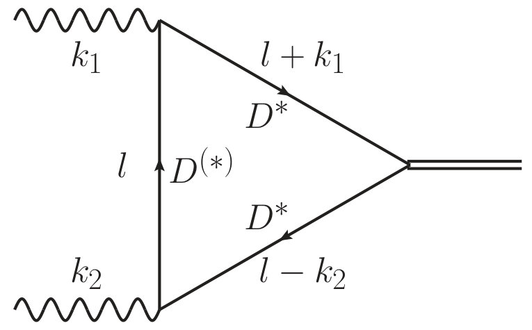 Figure 1
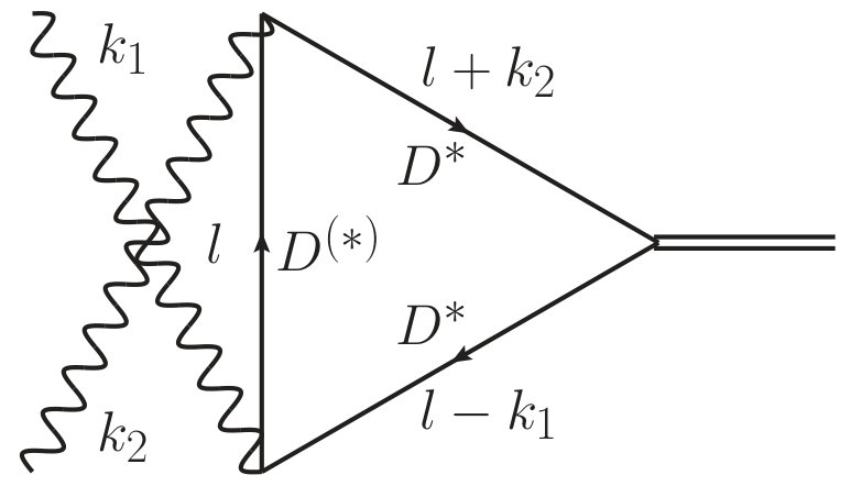 Figure 2
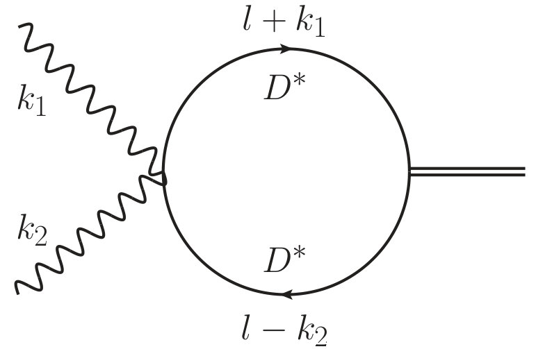 Figure 3
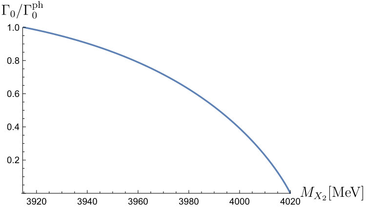 Figure 4
Peer Reviews
No public reviews on file for this paper yet. If you reviewed it on a platform where reviews are public (OpenReview, ICLR, NeurIPS, ICML), you can paste yours below so the community can read it here.
Videos
No videos yet. Explain this paper in a talk, walkthrough, or lecture? Add one.
aainstitutetext: Institut für Theoretische Physik II, Ruhr-Universität Bochum, D-44780 Bochum, Germanybbinstitutetext: Institute for Theoretical and Experimental Physics, B. Cheremushkinskaya 25, 117218 Moscow, Russiaccinstitutetext: Forschungszentrum Jülich, Institute for Advanced Simulation, Institut für Kernphysik and Jülich Center for Hadron Physics, D-52425 Jülich, Germanyddinstitutetext: National Research Nuclear University MEPhI, 115409, Kashirskoe highway 31, Moscow, Russiaeeinstitutetext: Moscow Institute of Physics and Technology, 141700, Institutsky lane 9, Dolgoprudny, Moscow Region, Russia
Can be the tensor partner of the ?
V. Baru c
C. Hanhart b,d,e
A. V. Nefediev
Abstract
It has been proposed recently (Phys. Rev. Lett. 115 (2015), 022001) that the charmoniumlike state named and suggested to be a scalar, is just the helicity-0 realisation of the tensor state . This scenario would call for a helicity-0 dominance, which were at odds with the properties of a conventional tensor charmonium, but might be compatible with some exotic structure of the . In this paper, we investigate, if such a scenario is compatible with the assumption that the is a molecular state — a spin partner of the treated as a shallow bound state. We demonstrate that for a tensor molecule the helicity-0 component vanishes for vanishing binding energy and accordingly for a shallow bound state a helicity-2 dominance would be natural. However, for the , residing about MeV below the threshold, there is no a priori reason for a helicity-2 dominance and thus the proposal formulated in the above mentioned reference might indeed point at a molecular structure of the tensor state. Nevertheless, we find that the experimental data currently available favour a dominant contribution of the helicity-2 amplitude also in this scenario, if spin symmetry arguments are employed to relate properties of the molecular state to those of the . We also discuss what research is necessary to further constrain the analysis.
1 Introduction
Among the most interesting and intriguing discoveries made in high energy physics in recent years, one should mention the discovery of many new hadrons lying above the open-flavour threshold both in the spectrum of charmonium and bottomonium — for reviews see, for example, Refs. Brambilla:2010cs ; Brambilla:2014jmp ; Abe:2010gxa ; Drutskoy:2012gt ; Asner:2008nq ; Lutz:2009ff . One of such states, the , was observed by the Belle Collaboration in the two-photon annihilation to the final state Uehara:2009tx , and the variety of options for the quantum numbers of this state was limited to just and . Later, the BaBar Collaboration reported that the angular distributions for the final-state leptons and pions emerging from the decays of the and favoured the option Lees:2012xs , so that this state is conventionally identified as the charmonium Liu:2009fe ; Olive:2016xmw — although this charmonium assignment was questioned in Refs. Guo:2012tv ; Olsen:2014maa . In Ref. Li:2015iga the was proposed to be a scalar molecule.
However, it was noticed recently Zhou:2015uva that the assumption used by BaBar in the data analysis, namely the assumption of a helicity-2 dominance for the tensor state, might not hold if the tensor state had an exotic structure. Acknowledging this, the state is called in the 2016 Review of Particle Physics (RPP) by the PDG Olive:2016xmw .
Historically, it was found long ago Alekseev that, in the two-photon decays of the positronium, only the helicity-2 amplitude contributes while the helicity-0 amplitude vanishes. This observation was later generalised to quarkonia Krammer:1977an ; Li:1990sx , and the helicity-0 amplitude was demonstrated to provide only a small relativistic correction to the dominating helicity-2 amplitude, in agreement with the findings of Ref. Alekseev . However, a similar analysis for exotic structures has not been done so far. Thus, it was pointed out in Ref. Zhou:2015uva that the helicity-2 dominance constraint may be relaxed in the data analysis if one assumes the to be some exotic state. The authors concluded that, for the helicity-0 amplitude comparable in magnitude with the helicity-2 one, the measured angular distributions could be reproduced under the assumption of quantum numbers of the suggesting that what was observed in Ref. Uehara:2009tx was simply the manifestation of the helicity-0 component of the tensor state known as .111Note that here and in what follows calling the state only means the definition of its quantum numbers and it does not imply a nature of this state, fully in line with the naming scheme defined in the RPP Olive:2016xmw . In this paper, we investigate if a prominent helicity-0 component is compatible with being a molecular state. To this end, we briefly repeat the theoretical arguments why one should expect a molecule to exist as a spin partner of the . Then we employ the Occam’s razor principle to identify the with this hypothetical spin-2 partner — the assumption allowing one to relate the effective coupling constant of the -wave transition to the experimentally measured binding energy of the . Equipped with this information, we study the properties of the in the two-photon annihilation processes.
One of the celebrated theoretical tools used in studies of hadronic states with heavy quarks is the Heavy-Quark Spin Symmetry (HQSS) which is based on the observation that, for , with denoting the quark mass, the strong interactions in the system are independent of the heavy quark spin. As a result, the hypothesis of the existence of a molecular state at one open-flavour threshold entails the existence of spin partner states at the neighbouring open-flavour thresholds, which differ by the heavy-quark spin orientation. For example, the idea of the existence of spin partners for the isovector bottomonium-like states and was put forward and investigated in Refs. Bondar:2011ev ; Voloshin:2011qa ; Mehen:2011yh . Although in case of the charm quark the ratio is sizable and one expects non-negligible corrections to the strict symmetry limit, constraints from HQSS can still provide a valuable guidance also in the charm sector and, in particular, for the Hidalgo-Duque:2013pva . Thus, it was argued in Refs. Nieves:2012tt ; Guo:2013sya that one should expect a shallow -wave bound state in the channel with the quantum numbers — the molecular partner of the conventionally denoted as . In Ref. Albaladejo:2015dsa , on the basis of an effective field theory with perturbative pions (X-EFT), the width of this state was estimated to be as small as a few MeV. Later, in Ref. Baru:2016iwj , an alternative EFT approach to the state was formulated considering pion exchanges nonperturbatively and it was concluded that the mass of this state might acquire a significant shift and that its width could be as large as several tens of MeV. In particular, its binding energy was found to constitute a few dozens MeV. An exploratory study of the possible impact of the genuine quarkonium on the formation of this molecular state is presented in Ref. Cincioglu:2016fkm and a further shift of the corresponding pole into the complex plane was argued to be possible.
Therefore, although the measured mass of the lies approximately 100 MeV below the threshold Olive:2016xmw , in the current research, we dare identify it with the — the tensor spin partner of the . Then, using the measured properties of the as an anchor, we trace the consequences of such an identification for the relative strength of the helicity-0 and helicity-2 amplitudes in the two-photon fusion processes proceeding through the formation of the state.
The paper is organised as follows: In Sec. 2 the amplitude for is decomposed into a complete set of four gauge invariant, mutually orthogonal tensor structures. We demonstrate how the helicity-0 and helicity-2 amplitudes can be expressed in terms of these tensors. In addition, the angular distributions of different two-photon annihilation processes proceeding via the state are evaluated and expressed in terms of the helicity amplitudes. We demonstrate that the leading helicity-0 amplitude contribution to the observables depends only on the coupling that may be estimated from the coupling, as explained in Subsec. 4.1, while the helicity-2 amplitude requires an additional contact term for renormalisation. Given that this contact term is unknown, the relative importance of the different helicity contributions for a tensor molecule cannot be fixed unambiguously without an additional experimental input — this insight is new to the best of our knowledge.
In order to proceed, we provide a complete evaluation of the analytic expressions derived for the helicity-0 amplitude (quoted in Appendix A) and involve additional plausible assumptions to extract the ratio of the helicity-2 to helicity-0 amplitudes directly from experimental data (for completeness, we also quote the explicit form of the helicity-2 amplitude in Appendix B). To this end, in Subsec. 4.1, we employ HQSS and the molecular interpretation for the and its spin partners to express the coupling constants of the spin-2 and spin-0 states to the meson pairs through the binding energy of the and, in Subsec. 4.2, we confront the evaluated helicity-0 contribution to the two-photon decay width with the experimental data to draw conclusions on the relative importance of the helicity-0 and helicity-2 amplitudes. Our results point towards a helicity-2 dominance for the spin-2 heavy-quark spin symmetry partner of the , although, as stressed in Sec. 5, due to limited information currently available about this state, this conclusion is subject to potentially large uncertainties. Such a helicity-2 dominance is at odds with the need expressed in Ref. Zhou:2015uva that, in order to be consistent with a state, the angular distributions of the various two-photon annihilation processes call for a sizable helicity-0 contribution. Therefore, our study suggests that if the were indeed just a realisation of the state , its properties seem to be not consistent with its being the predicted spin partner of the . On the other hand, if the is a molecular partner of the , it is presumably the scalar state. We also discuss how additional data would allow one to draw more firm conclusions.
2 The amplitude
2.1 Electric and magnetic contributions
The amplitude of the fusion process can be written in the form
[TABLE]
where , are the first and the second photon polarisation vector, respectively, and is the polarisation tensor which obey the standard constraints,
[TABLE]
There are two mechanisms responsible for the interaction with the electromagnetic field which produce two types of vertices: the electric vertices and the magnetic ones. The covariant form of the electric () vertex reads Guo:2014taa
[TABLE]
where is the electric part of the interaction Lagrangian and is the charge matrix corresponding to the isospin doublet ; satisfies the Ward identity,
[TABLE]
where the propagator and its inverse form are
[TABLE]
An additional electric seagull-like contact vertex reads
[TABLE]
The Lagrangian describing the leading magnetic interaction between the and mesons takes the form
[TABLE]
where is the four-velocity of the heavy quark () and the magnetic moment matrices for the transitions read
[TABLE]
with being the light-quark charge matrix, and and being the charmed-quark mass and charge, , respectively. Here the leading -terms account for the nonperturbative light-flavour cloud in the charmed meson and the subleading terms proportional to come from the magnetic moment of the charm quark. In what follows we use the values Hu:2005gf
[TABLE]
The nonrelativistic reduction of Eq. (6) yields the Lagrangian which agrees with that given in Ref. Hu:2005gf .
Then, the magnetic and () vertices read Guo:2014taa
[TABLE]
and
[TABLE]
respectively. Both vertices are manifestly transversal with respect to the photon momentum .
The diagrams contributing to the fusion amplitude are depicted in Fig. 1. The first two diagrams acquire contributions from both electric and magnetic vertices given in Eq. (3) and in Eqs. (9), (10), respectively, while the last, fish-like diagram is purely electric — see the vertex given in Eq. (5). It has to be noticed that the dominating contribution to this amplitude comes from the triangle diagrams with two magnetic vertices. Indeed, the magnetic photon emission vertices contain the matrices (7) which provide large numeric enhancement factors due to the isospin traces along the loop with two such vertices,
[TABLE]
which are to be confronted with the factors
[TABLE]
for the triangle diagrams with one and with no magnetic vertex, respectively. Here the averaged mass MeV was used for the estimate. In the evaluation above it was used that the is an isosinglet state.
2.2 Helicity decomposition
There are in total four independent, gauge invariant two-photon tensors, which one may choose as
[TABLE]
The various terms in the interaction Lagrangian for the spin-2 field coupled to two photons are expressed as contractions of the above structures with the tensor . Furthermore, the () in Eqs. (13)-(16) stand for scalar functions that parametrise the dynamics of the decay.222Hereinafter we stick to the on-shell photons, so that (, ). The set (13)-(16) exhausts all possible second-order tensor structures built with the help of the two photon field tensors and symmetric with respect to the permutation. This guarantees that the set of the structures (13)-(16) is complete in the given class of tensors.
In order to perform the helicity decomposition of the amplitude (1) we introduce a quartet of tensors based on the structures from Eqs. (13)-(16),
[TABLE]
which are mutually orthogonal and normalised,
[TABLE]
In addition, they are symmetric and transversal,
[TABLE]
The set (17)-(20) is complete, so that the tensor defined in Eq. (1) can be decomposed as
[TABLE]
where for later convenience the couplings are pulled out of the definition of the coefficients . Gauge invariance and the symmetry of the tensor amplitude (23) are obvious due to the properties listed in Eq. (22). Therefore, the entire information about the amplitude (1) is encoded in the functions .
3 Two-photon annihilation through the
Consider the two-photon annihilation process into various final states which proceeds through the formation of the . Then, the tensor from Eq. (1) is to be contracted with the propagator taken in the standard form,
[TABLE]
where
[TABLE]
[TABLE]
and is the width.
It has to be noticed, however, that not all coefficients contribute to the amplitude of the process under study, when the two-photon tensor from Eq. (23) is contracted with the polarisation tensor with any polarisation . Indeed, for convenience, let us define two orthogonal combinations of the basis tensors and , namely, and . Then, using the properties of the polarisation tensor summarised in Eq. (2) and the momentum conservation law , it is staightforward to see that
[TABLE]
so that only the coefficient and the combination contribute to the amplitude of the two-photon annihilation process which proceeds through the formation of the tensor state .
3.1 annihilation
The amplitude of the two-photon fusion reaction reads
[TABLE]
where and are the momenta of the two mesons in the final state, respectively, and the vertex is taken in the form
[TABLE]
The kinematics of the process in the centre-of-mass frame is such that ( and are unit vectors)
[TABLE]
where . Then, the angular distribution is given in terms of .
Taking Eqs. (23) and (27) together and using the explicit form of the basis tensors (17)-(20), it is straightforward to find for the differential cross section ()
[TABLE]
where we introduced the helicity-0 and helicity-2 amplitudes,
[TABLE]
with the same constant, and the quantities and are given by the Wigner functions with and with the helicity equal to 0 and 2, respectively,
[TABLE]
Both functions are normalised to unity as
[TABLE]
3.2 annihilation
Consider the annihilation reaction accompanied by the subsequent three-pion decay and by the dilepton decay . The kinematics of the reaction simplifies considerably if one notices that, at , the and the are quite slow because the annihilation proceeds only about 35 MeV above the threshold, which corresponds to a centre-of-mass momentum MeV. Therefore, neglecting corrections suppressed by the small factors and , we consider both and at rest.
The angular distribution in , defined as the angle between the collision axis of the initial photons and the momentum of the positively charged lepton , follows from the contraction
[TABLE]
where the tensor is given by the spectral density of the meson at rest, that is by
[TABLE]
and the tensor is
[TABLE]
with
[TABLE]
where we neglected the lepton mass as .
It is straightforward then to find that ()
[TABLE]
where the distribution functions
[TABLE]
are normalised to unity,
[TABLE]
and relations (31) hold for the helicity amplitudes and . The distribution (38) agrees with the formulae derived from the general principles of the rotational symmetry — see Eqs. (12) and (13) of Ref. Rosner:2004ac .
Similarly, the angular distribution in , defined as the angle between the collision axis of the initial photons and the normal vector to the plane formed by the three pions originated from the decay ()), follows from the contraction
[TABLE]
where the tensor is now defined as
[TABLE]
and the tensor is given by the spectral density of the at rest, that is by
[TABLE]
Then, at ,
[TABLE]
where, as before, the same coefficients from Eq. (31) appear and the distribution functions
[TABLE]
are normalised to unity,
[TABLE]
Distribution (44) agrees with Eqs. (12) and (14) of Ref. Rosner:2004ac .
3.3 Evaluation of the helicity amplitudes
From Eqs. (30), (38), and (44) one can see that, in agreement with the natural expectations, the angular distribution takes a universal form,
[TABLE]
where the functions and depend on the particular final state, as derived above, and are given by the normalised helicity-0 and helicity-2 distribution, respectively Rosner:2004ac ; Zhou:2015uva . Similarly, in Eq. (47) stands for an overall constant depending on the final state in the two photon fusion process. The dynamics is encoded in the helicity amplitudes and defined in Eq. (31). Therefore, one can conclude that the tensor structures (17)-(19) correspond to the helicity equal to 0 while the tensor structure (20) corresponds to the helicity equal to 2. The form of the angular distribution given by Eq. (47) depends on the relative strength of the coefficients, and we may define the ratio
[TABLE]
to rewrite the differential cross section (47) in the form
[TABLE]
where corresponds to the total cross section evaluated solely for the helicity-0 amplitude.
An explicit evaluation of the loop integrals yields that their contributions to the coefficients are divergent and thus call for an additional counter terms to render the amplitude well defined. However, due to the property (see Eq. (2)), the structure (13) and correspondingly the coefficient does not contribute to observables and, as was demonstrated above, the structures (14) and (15) contribute to the transition amplitude in the combination which is finite — see the Appendix A for the explicit form of the amplitude . This observation suggests that local counterterms for this contribution appear only at a higher order. In particular, the leading-order short-range contributions to the two-photon decay proceeding via excitation of two vector mesons in the intermediate state (for example, ) or via the quarkonium component of the wave function contribute to the helicity-2 amplitude only. Therefore, once the coupling is fixed via its connection to the coupling (see Eqs. (53) below), the helicity-0 contribution comes as a prediction of the model. On the other hand, to quantify the helicity-2 amplitude, a counter term needs to be fixed by some data. This shows that the relative importance of the two helicity components is, in general, not fixed by the structure. On the other hand, as will be shown below, for a vanishing binding energy the contribution of the helicity-0 amplitude vanishes, and a helicity-2 dominance in the observables appears to be natural, in analogy to regular charmonia.
In order to proceed we now calculate the helicity-0 component within the molecular model outlined and then use data to fix the ratio introduced in Eq. (48).
4 Ratio of the helicity amplitudes from data
4.1 The coupling
Under the assumption that the is a molecule, its dominating decay mechanism proceeds through the -wave vertex followed by -meson loops. In order to estimate the coupling constant , we employ the assumption that the is a spin partner of the and, therefore, they both appear as members of the same superfield — see, for example, Ref. Mehen:2015efa ,
[TABLE]
where the nonrelativistic fields , , and describe the , the , and the hypothetical scalar molecular state , respectively. The field (50) interacts with the vector and pseudoscalar heavy-light mesons as
[TABLE]
where
[TABLE]
with () and () denoting the vector and pseudoscalar meson (antimeson) states, respectively.
Substituting Eqs. (50) and (52) into Eq. (51) and taking traces, one gets relations between the nonrelativistic couplings consistent with HQSS,
[TABLE]
where, in our calculation, and correspond to the and meson, respectively.333Note that due to the -wave character of the vertex defined in Eq. (28) the coupling is not related to the couplings that appear in Eq. (53).
To proceed, we use the state as the anchor since, in the molecular scenario, its coupling constant to the pair can be evaluated through its measured binding energy as Guo:2013nza (see also Refs. Landau ; Weinberg:1965zz ; Baru:2003qq for more general discussions)
[TABLE]
where and stand for the and -meson masses, respectively,444Strictly speaking, in the HQSS limit, the and mesons are degenerate in mass, so that one cannot distinguish between and . For definiteness, up to the corrections to the heavy-quark limit, we define the reduced mass as given in Eq. (54) and use it in the other coupling constants as well — see Eq. (55) below. and the ellipsis denotes the terms suppressed as , with being the inverse range of the force. Thus, the nonrelativistic coupling constants for the scalar and tensor spin partners of the read
[TABLE]
Then the interaction Lagrangian with relativistic vertices can be written as
[TABLE]
where
[TABLE]
and () stands for the mass of the resonance with the total spin . To arrive at Eq. (4.1), we used the relation between the relativistic and nonrelativistic coupling constants, namely
[TABLE]
4.2 Two-photon decay width and the ratio of the helicity amplitudes
Consider the two-photon decay of the molecule which, due to the -invariance, is described by the amplitude (1). Then the differential width can be written in a form similar to Eq. (49). Since the angular distributions and are normalised to unity, the angular integration yields
[TABLE]
where, as before, denotes the width evaluated solely for the helicity-0 amplitude. We stress again that, within the model at hand, this piece is fixed in terms of the coupling constant of the to .
Using the explicit form of the amplitude (23) and the value of the coupling constant from Eq. (4.1), one can find that (the binding energy is measured in MeV)
[TABLE]
which comes out as a prediction of the model used.555The calculations were performed with the help of Wolfram Mathematica supplied with the FeynCalc Mertig:1990an ; Shtabovenko:2016sxi and Package-X Patel:2015tea packages. In addition, for a cross check, the LoopTools package was employed Hahn:1998yk .
In order to proceed, one needs an estimate of the binding energy. The most up-to-date value of the mass reads Olive:2016xmw
[TABLE]
which gives for the
[TABLE]
Since the central value of the is basically consistent with zero, for an estimate, we take the upper bound MeV. Then, Eq. (60) yields
[TABLE]
We may now employ this result in Eq. (59) to extract the ratio from the data on . Unfortunately, the existing data are rather uncertain and, in addition, the analysis may implicitly include a particular assumption about the quantum numbers of the state and/or about a particular helicity dominance for it, like it was done in Ref. Lees:2012xs . We, therefore, consider several results of different experimental measurements simultaneously to reliably estimate the two-photon decay width .
We start from the Belle result Uehara:2005qd 666While Belle calls this state we here employ the PDG naming scheme and call it
[TABLE]
and, following Ref. Zhou:2015uva , identify the tensor state with . Then we use the fact that its total width is largely saturated by the mode, so, for an estimate, it is natural to set Olive:2016xmw . This leads to the estimate
[TABLE]
An alternative way to extract the two-photon width is to use the measurements of the . In particular, the Belle result from Ref. Uehara:2009tx reads
[TABLE]
while BaBar gives Lees:2012xs
[TABLE]
Thus, for the estimate, we take an averaged value
[TABLE]
which arises if the above measurements for the quantum numbers are used.
Now, to extract the width from Eq. (68), we use the experimental value for the product of the BF’s
[TABLE]
which is quoted by the PDG Olive:2016xmw as the average between the BaBar and Belle measurements — see Refs. delAmoSanchez:2010jr and Abe:2004zs , respectively. The value (69) is also consistent with another BaBar measurement reported in Ref. Aubert:2007vj .
If, in addition, we assume that the production branching falls into the ball park of the BF’s for the production of other known charmonia in -meson weak decays Olive:2016xmw , that is, that it constitutes a few units times , then it is straightforward to arrive at the estimate
[TABLE]
which allows one to extract the width from (68) to be
[TABLE]
which is fairly consistent with the independent estimate of Eq. (65).
As an additional consistency check we notice that, starting from the two-photon decay width of the charmonium Ablikim:2012xi ,
[TABLE]
and taking into account that it is natural to expect a few times smaller value of the width for the excited tensor state, one qualitatively re-arrives at the estimate (65).
Now, with the theoretical estimate of the helicity-0 contribution given in Eq. (63) and with the phenomenological estimate for the total two-photon width of Eq. (65) at hand, we are in a position to estimate the value of the ratio employing Eq. (59). This yields
[TABLE]
where, as it was explained above, to arrive at this estimate we used the upper bound on the binding energy . In the limit , the ratio grows as .
5 Discussion, Disclaimers and possible future improvements
The result of Eq. (73) suggests a strong helicity-2 amplitude dominance in the two-photon decay of a 2*++* molecular state in the mass range of 3915 MeV under the assumption that this state is the spin partner of the , the latter assumed to be a bound state. Moreover, as one can see from Fig. 2, had the mass of the state been located closer to the threshold, strong cancellations between the contributions to the helicity-0 amplitude from the diagrams depicted in Fig. 1 with the intermediate and particles would have taken place thus damping the helicity-0 contribution to the two-photon width. As a consequence, the state would have been almost entirely dominated by the helicity-2 amplitude, unless it had completely decoupled from . Thus the behaviour were analogous to that of Ref. Li:1990sx for the genuine charmonium assignment and Refs. Alekseev ; Krammer:1977an for the positronium. On the other hand, as shown in Ref. Zhou:2015uva , the angular distributions measured by BaBar are consistent with the being either a tensor state with the large helicity-0 contribution or a scalar state. Based on the analysis presented in this paper, one is, therefore, tempted to conclude that if the is indeed the helicity-0 contribution of the nearby tensor state, which requires an exotic structure of the latter, it is not the spin partner of the .
However, there were various assumptions used to arrive at the estimate of Eq. (73). First of all, there are quite some uncertainties in the estimate for given in Eq. (65). Clearly, this can be improved by more refined measurements of this quantity. Next, in order to employ Eq. (54), we needed to assume the to be a bound state. However, current data on the are also compatible with a virtual state Hanhart:2007yq and then Eq. (54), derived from the normalisation of the bound state wave function, does not hold anymore. In the case of a virtual state, the extraction of the coupling constant could be done directly by fitting the experimental line shapes along the lines of Refs. Hanhart:2007yq ; Kang:2016jxw , which, however, requires high-resolution and high-statistics data not available at present. In this context, it is also important to remember that the data currently available for channel were subject to a kinematic fit that might have distorted the line shape Stapleton:2009ey .
In order to relate the coupling of the to that of its spin partner we needed to use heavy-quark spin symmetry. However, in the charm sector, there might occur a significant spin symmetry violation, since is not a small parameter. Furthermore, especially for the , there might be significant spin symmetry violating contributions induced by the sizeable mass difference of the and intermediate states Baru:2016iwj . In order to improve on this piece of the calculation, a better understanding of the impact of spin symmetry violations on spin multiplets is required. In addition, from the theoretical side, the role of a mixing with states needs to be better understood Cincioglu:2016fkm — see also Ref. Hammer:2016prh where this issue is approached from a different angle. Clearly, these are major tasks that need both further calculations as well as further data, especially for additional quantum numbers Cleven:2015era , not only in the charm sector but also in the bottom sector Bondar:2016hva . In this sense, the study presented in this work can be regarded as an additional step towards a concise and complete understanding of the heavy meson spectrum above the open-flavour threshold.
6 Conclusions
Even almost 15 years after the discovery of the the heavy-meson spectrum above the open-flavour thresholds still raises a lot of questions. Many proposals are put forward to explain the large number of unusual states discovered in the mean time and so far no coherent picture is on the horizon. In order to improve the situation, it appears necessary to better understand the implications of the heavy-quark spin symmetry and its violations on the spectrum of heavy hadrons which are very different in the different scenarios Cleven:2015era .
In this paper, we treat the as a molecule to investigate if within this scenario it could indeed be the tensor state known as — an identification that calls for a prominent helicity-0 component in the wave function of the state Zhou:2015uva . To this end, we study the two-photon annihilation processes proceeding through the and evaluate the two-photon decay width of this state. We find that, for such a molecule, the helicity-0 component vanishes as the binding energy tends to zero while the helicity-2 piece (which contains an unknown counter term) is expected to be finite, unless the completely decouples from the channel in this limit. Thus, it appears natural that shallow bound states share the feature of a helicity-2 dominance with regular charmonia. However, the state at hand is located about 100 MeV below the threshold and, therefore, no a priori conclusion about the relative importance of the helicity amplitudes is possible.
In order to proceed, we investigate whether or not the could be the spin-2 partner of the which is assumed to be a bound state. To this end, we evaluate the contribution of the helicity-0 amplitude to the two-photon decay width of the , which is finite and comes out as a prediction of the model once spin symmetry is used to connect the effective coupling constant of the to that of the . We argue that the experimental data presently available for the mass and for the two-photon decay width of the tensor charmonium favour a scenario in which the contribution of the helicity-2 amplitude dominates over the helicity-0 one, similarly to the case of the genuine charmonium.
In summary, if the is the hadronic molecule that should exist as a spin partner of the , current data favour a scalar assignment for this state. On the other hand, if the were indeed dominated by the helicity-0 contribution of the nearby tensor state, its nature would require some exotic interpretation related neither with regular quarkonia nor with the spin partner of the . However, it needs to be acknowledged that the analysis performed is subject to several uncertainties which are difficult to quantify, given the present status of the experimental data as well as our theoretical understanding of the charmonium spectrum above the open flavour thresholds. We also outline how those uncertainties could be reduced in future studies.
Acknowledgements.
The authors are grateful to F.-K. Guo and to R. V. Mizuk for enlightening discussions. This work is supported in part by the DFG and the NSFC through funds provided to the Sino-German CRC 110 “Symmetries and the Emergence of Structure in QCD” (NSFC Grant No. 11261130311). Work of A. N. was performed within the Institute of Nuclear Physics and Engineering supported by MEPhI Academic Excellence Project (contract No 02.a03.21.0005, 27.08.2013). He also acknowledges support from the Russian Foundation for Basic Research (Grant No. 17-02-00485). Work of V. B. is supported by the DFG (Grant No. GZ: BA 5443/1-1).
Appendix A Helicity-0 amplitude
In this Appendix we collect explicit expressions for the contributions and defined in Eq. (23) (here the particle which appears in the middle propagates between the photon emission vertices) to the helicity-0 amplitude from Eq. (31) which stem from the triangle diagrams depicted in Fig. 1. The individual contributions read (here )
[TABLE]
where , stands for the renormalisation scale in the dimensional regularisation scheme, and is Euler’s constant. Furthermore,
, is the scalar Passarino-Veltman function, which is finite (for example, ), and the coefficients and read
[TABLE]
Here , , , and stand for the isospin traces taken for the triangle diagram with the meson propagator between the photon emission vertices. The superscripts , , and denote two magnetic, one magnetic plus one electric, and two electric photon emission vertices, respectively. Then, with the help of the explicit form of the matrices (see Eq. (7)) and the matrix (see below Eq. (3)) one readily finds
[TABLE]
We emphasise once more that while both functions and diverge, their combination which contributes to is finite
[TABLE]
where the coefficients read and .
Appendix B Helicity-2 amplitude
For completeness, in this Appendix we collect explicit expressions for the contributions defined in Eq. (23) (as in Appendix A, in this notation, the particle which appears in the middle propagates between the photon emission vertices) to the helicity-2 amplitude from Eq. (31) which stem from the triangle diagrams depicted in Fig. 1. The individual contributions are (here )
[TABLE]
and the coefficients and read
[TABLE]
We note that both and contain nonvanishing divergent pieces (proportional to — see Appendix A for the definition of ) which do not cancel each other in the total helicity-2 amplitude and which, therefore, call for a contact term for renormalisation.
The reference list from the paper itself. Each links out to its DOI / PubMed record.
- 1(1) N. Brambilla et al., Heavy quarkonium: progress, puzzles, and opportunities , Eur. Phys. J. C 71 (2011) 1534 , [ 1010.5827 ]. · doi ↗
- 2(2) N. Brambilla et al., QCD and Strongly Coupled Gauge Theories: Challenges and Perspectives , Eur. Phys. J. C 74 (2014) 2981 , [ 1404.3723 ]. · doi ↗
- 3(3) Belle-II collaboration, T. Abe et al., Belle II Technical Design Report , 1011.0352 .
- 4(4) A. G. Drutskoy, F.-K. Guo, F. J. Llanes-Estrada, A. V. Nefediev and J. M. Torres-Rincon, Hadron physics potential of future high-luminosity B-factories at the Υ ( 5 S ) Υ 5 𝑆 \Upsilon(5S) and above , Eur. Phys. J. A 49 (2013) 7–32 , [ 1210.6623 ]. · doi ↗
- 5(5) D. M. Asner et al., Physics at BES-III , Int. J. Mod. Phys. A 24 (2009) S 1–794, [ 0809.1869 ].
- 6(6) PANDA collaboration, M. F. M. Lutz et al., Physics Performance Report for PANDA: Strong Interaction Studies with Antiprotons , 0903.3905 .
- 7(7) Belle collaboration, S. Uehara et al., Observation of a charmonium-like enhancement in the γ γ → ω J / ψ → 𝛾 𝛾 𝜔 𝐽 𝜓 \gamma\gamma\to\omega J/\psi process , Phys. Rev. Lett. 104 (2010) 092001 , [ 0912.4451 ]. · doi ↗
- 8(8) Ba Bar collaboration, J. P. Lees et al., Study of X ( 3915 ) → J / ψ ω → 𝑋 3915 𝐽 𝜓 𝜔 X(3915)\to J/\psi\omega in two-photon collisions , Phys. Rev. D 86 (2012) 072002 , [ 1207.2651 ]. · doi ↗