Localized Stress Fluctuations Drive Shear Thickening in Dense Suspensions
Vikram Rathee, Daniel L. Blair, Jeffery S. Urbach

TL;DR
This study reveals that shear thickening in dense suspensions is driven by localized regions of high viscosity that dynamically form and dissolve, linking microscopic particle interactions to macroscopic flow behavior.
Contribution
It uncovers the physical mechanism of shear thickening as dynamic localized viscosity regions, connecting microscopic heterogeneities to bulk rheology.
Findings
Localized high-viscosity regions increase with shear stress.
Spatial extent of heterogeneities depends on gap between surfaces.
Shear thickening results from transitions between low and high viscosity phases.
Abstract
The mechanical response of solid particles dispersed in a Newtonian fluid exhibits a wide range of nonlinear phenomena including a dramatic increase in the viscosity \cite{1-3} with increasing stress. If the volume fraction of the solid phase is moderately high, the suspension will undergo continuous shear thickening (CST), where the suspension viscosity increases smoothly with applied shear stress; at still higher volume fractions the suspension can display discontinuous shear thickening (DST), where the viscosity changes abruptly over several orders of magnitude upon increasing applied stress. Proposed models to explain this phenomenon are based in two distinct types of particle interactions, hydrodynamic\cite{2,4,5} and frictional\cite{6-10}. In both cases, the increase in the bulk viscosity is attributed to some form of localized clustering\cite{11,12}. However, the physical…
Click any figure to enlarge with its caption.
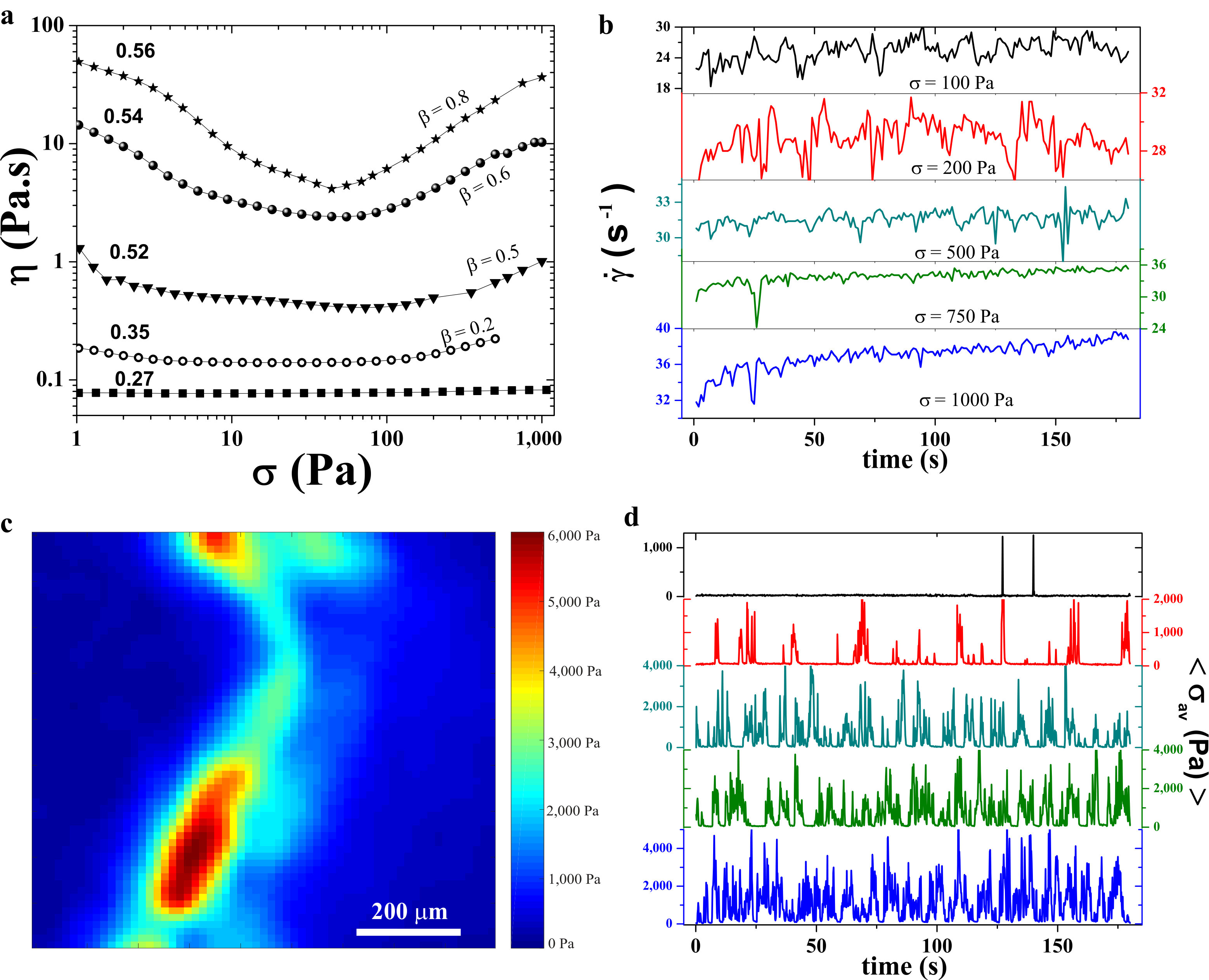 Figure 1
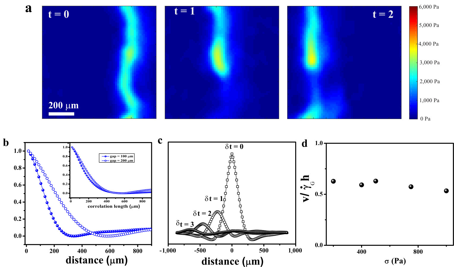 Figure 2
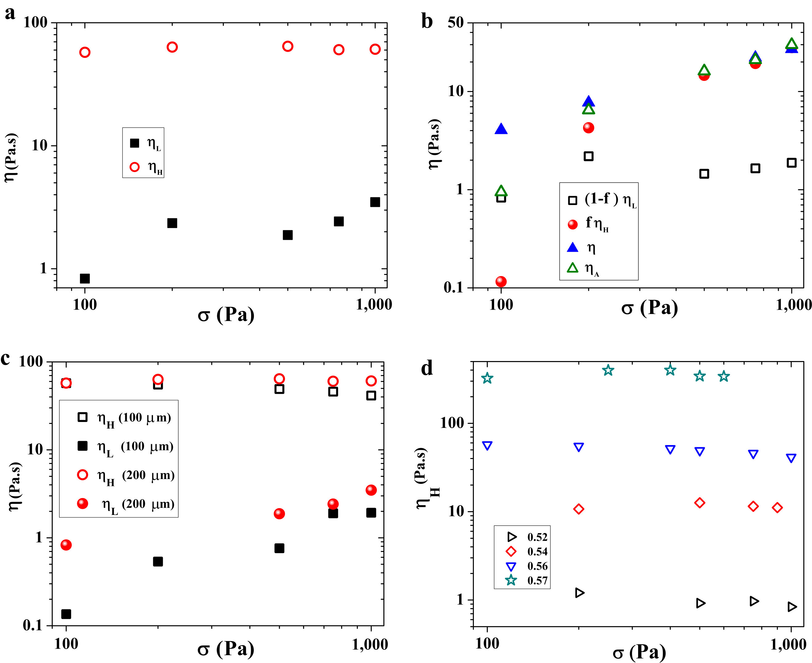 Figure 3
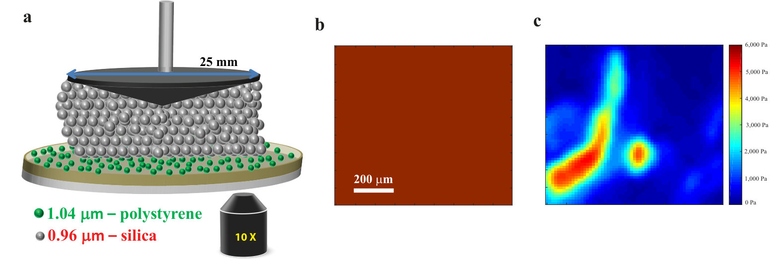 Figure 1
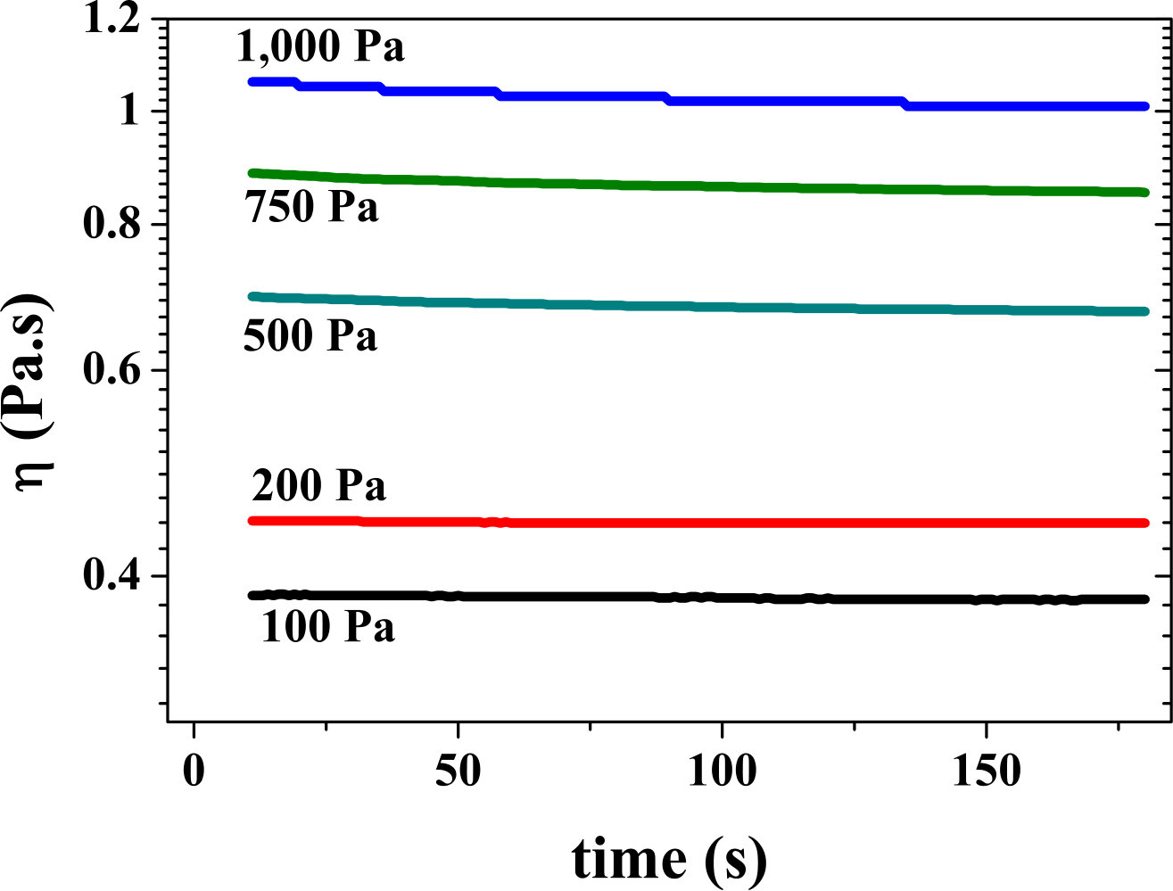 Figure 2
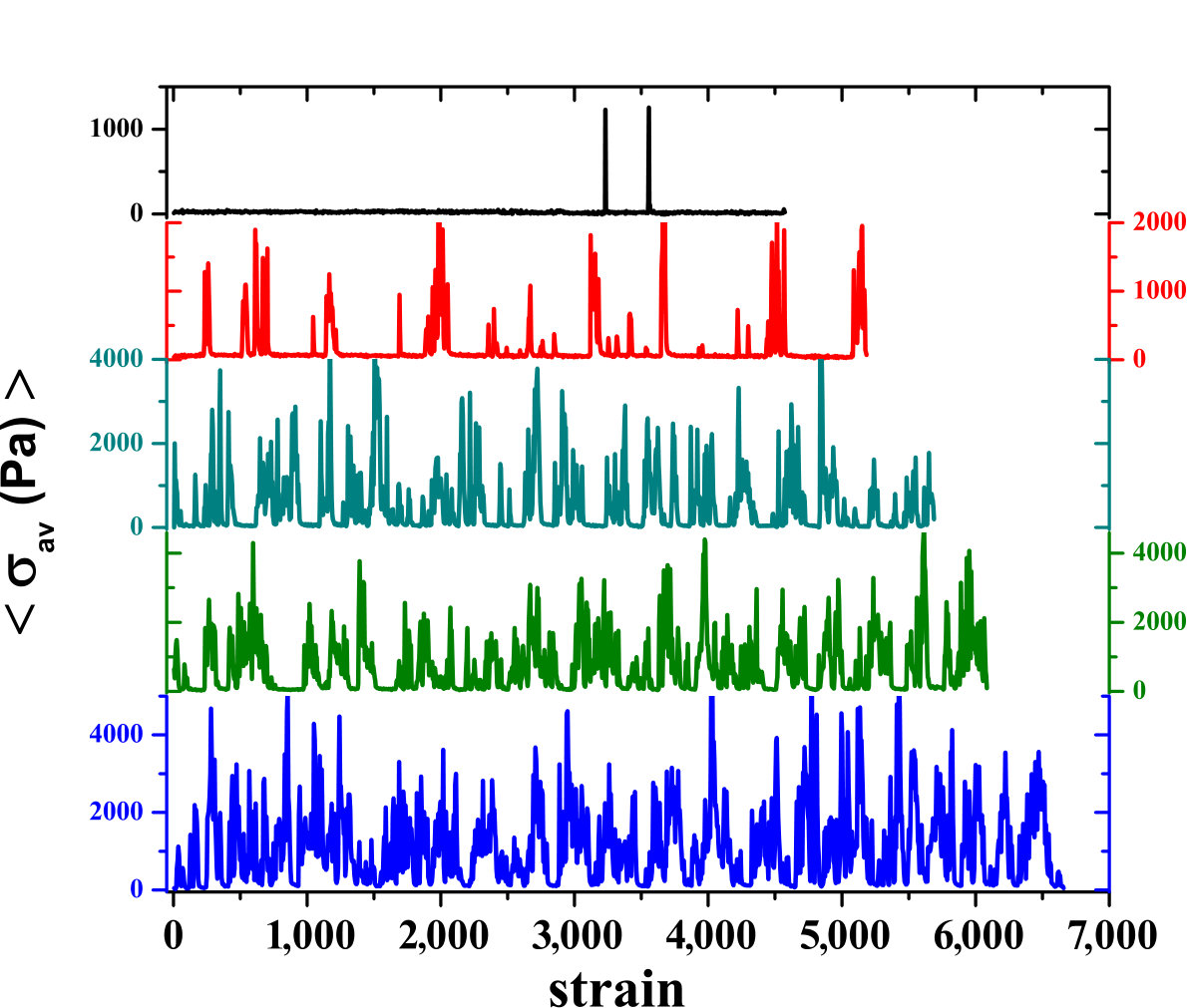 Figure 3
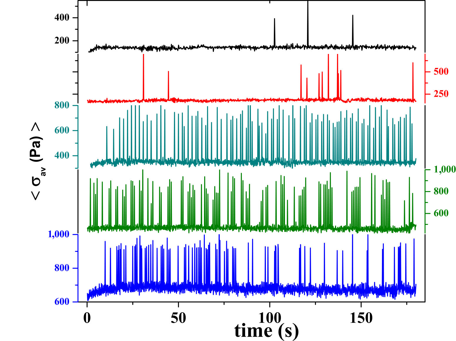 Figure 4
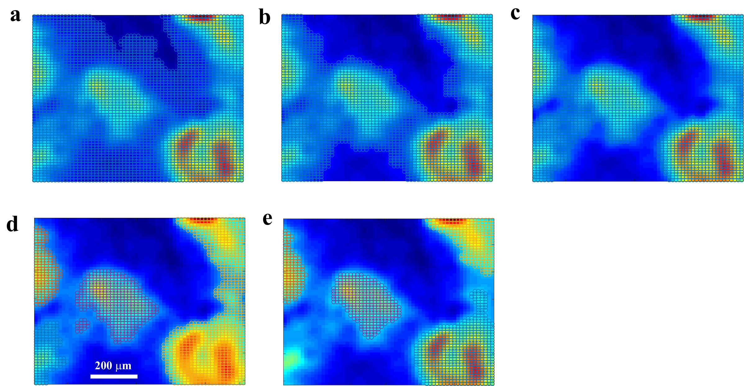 Figure 7
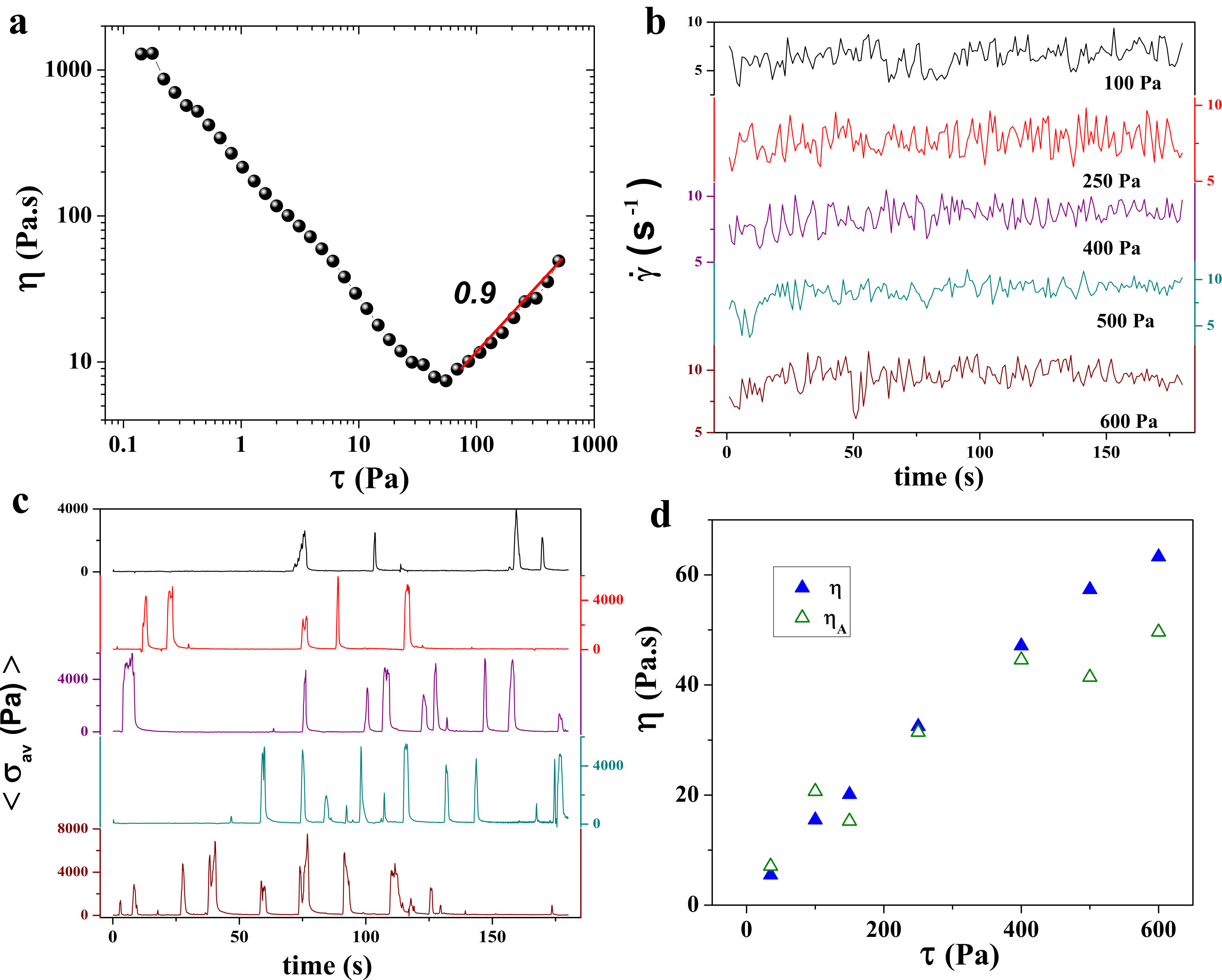 Figure 8
Peer Reviews
No public reviews on file for this paper yet. If you reviewed it on a platform where reviews are public (OpenReview, ICLR, NeurIPS, ICML), you can paste yours below so the community can read it here.
Videos
No videos yet. Explain this paper in a talk, walkthrough, or lecture? Add one.
Taxonomy
TopicsMaterial Dynamics and Properties · Rheology and Fluid Dynamics Studies · Granular flow and fluidized beds
Localized Stress Fluctuations Drive Shear Thickening in Dense Suspensions
Vikram Rathee1
Daniel L. Blair1 & Jeffrey S. Urbach1
{affiliations}
Dept. of Physics and Institute for Soft Matter Synthesis and Metrology, Georgetown University, Washington, DC.
Email: [email protected]; [email protected]; [email protected].
The mechanical response of solid particles dispersed in a Newtonian fluid exhibits a wide range of nonlinear phenomena including a dramatic increase in the viscosity [1, 2, 3] with increasing stress. If the volume fraction of the solid phase is moderately high, the suspension will undergo continuous shear thickening (CST), where the suspension viscosity increases smoothly with applied shear stress; at still higher volume fractions the suspension can display discontinuous shear thickening (DST), where the viscosity changes abruptly over several orders of magnitude upon increasing applied stress. Proposed models to explain this phenomenon are based in two distinct types of particle interactions, hydrodynamic[2, 4, 5] and frictional [6, 7, 8, 9, 10]. In both cases, the increase in the bulk viscosity is attributed to some form of localized clustering [11, 12]. However, the physical properties and dynamical behavior of these heterogeneities remains unclear. Here we show that continuous shear thickening originates from dynamic localized well defined regions of particles with a high viscosity that increases rapidly with concentration. Furthermore, we find that the spatial extent of these regions is largely determined by the distance between the shearing surfaces. Our results demonstrate that continuous shear thickening arises from increasingly frequent localized discontinuous transitions between coexisting low and high viscosity Newtonian fluid phases. Our results provide a critical physical link between the microscopic dynamical processes that determine particle interactions and bulk rheological response of shear thickened fluids.
Recent experimental work suggests that both frictional and hydrodynamic lubrication forces play a significant role in CST [11, 12]. Wyart and Cates (W-C) have introduced a phenomenological model in which the shear thickening arises from a transition from primarily hydrodynamic interactions when the applied stress is substantially below a critical stress, , to primarily frictional interactions when . While the W-C model and its extensions can reproduce the measured average rheological behavior [8, 12], it does not account for observed temporal fluctuations in bulk viscosity or shear rate [13, 14], or local density differences observed in magnetic resonance studies of a corn-starch suspension [15]. Similarly, numerical simulations have revealed stress fluctuations at the particle level and at larger scales [14]. These results indicate that the spatiotemporal dynamics of shear thickening includes complexity that cannot be captured by mean field models like W-C.
Here we describe the result of directly measuring the local stresses transmitted to one surface of a sheared suspension using Boundary Stress Microscopy (BSM), a technique we developed that applies traction force microscopy to rheological experiments[16]. To perform BSM measurements, we replace the bottom rheometer plate with a glass slide coated with a thin, uniform elastomer of known elastic modulus with a sparse coating of bound fluorescent microspheres. We use the measured displacements of the microspheres to determine the stresses at the boundary with high spatial and temporal resolution (see Methods). We apply BSM to a suspension of silica colloidal particles with radius m suspended in an index matched mixture of glycerol and water. Rheology is performed using a 25mm cone-plate geometry to ensure a uniform average shear rate, with a fixed, flat bottom surface and an angled cone that defines the top surface of the sample and rotates in response to the torque applied by the rheometer (Supplementary Fig. 1a).
The rheological response of these suspensions to increasing stress is similar to the typical shear thickening behavior previously reported [1]. Specifically, we observe that the measured viscosity as a function of the applied shear stress , is strongly non-Newtonian for concentrations , where and are the total particle volume and the system volume respectively (Fig. 1a). When , we observe a moderate shear thinning for Pa, followed by a Newtonian plateau and finally shear thickening, indicated by a small increase in above an onset or critical shear stress (Fig. 1a, open circles). For concentrations of , strong thinning is followed by an increase in the plateau viscosity and above , scales with an exponent () that increases with (Fig. 1a). As previously reported, does not show significant concentration dependence [21, 12]. For this system we observe discontinuous thickening at ; here we focus on concentrations below this value.
While the temporally averaged response provides a bulk picture of CST, the time resolved rheology reveals substantial fluctuations. Figure 1b shows the strain rate reported by the rheometer as a function of time for suspensions at with a constant applied stress for 180 seconds. The fluctuations represent variations in the shear rate as the rheometer adjusts the rotation rate of the cone that defines the upper boundary of the suspension in order to maintain a constant total stress. For stresses below the onset of shear thickening, Pa, fluctuations are absent (not shown). We observe that as the stress is increased above the rapid increase in the viscosity is associated with a marked increased in the magnitude of the fluctuations (Fig. 1b). Below , we do not see any fluctuations in (Supplementary Fig. 2), although does increase substantially above .
In addition to measuring the system-averaged viscosity versus time under constant stress, we measure the spatially resolved boundary stresses at specific locations in the rheometer using BSM. Below the displacements of the elastic substrate, and therefore the calculated boundary stresses, are spatially and temporally uniform (Supplementary Fig. 1b). However, above and for concentrations , we observe the appearance of localized surface displacements that are much higher than the average displacement (Supplementary Fig. 1c).
Figure 1c shows an example of the spatial map the component of the boundary stress in the velocity direction calculated from the measured displacement fields. The field of view is m and the regions of high stresses are large compared to the particle size. Moreover, the total area imaged represents of the total surface area of the system, indicating that the spatial scale of the stress variation is much smaller than the scale of the lateral system size (25 mm). Images at higher spatial resolution do not reveal any any significant stress variations on smaller length scales, down to our instrumental resolution of m [16].
The regions of high stress at the boundary appear with increasing frequency as the applied stress in increased above . This can be clearly seen in a time series of the average stress in each image (see Fig. 1d). At applied stresses just above , most images do not exhibit high stress regions, and thus have a small average stress. High stress fluctuations are clearly separated from the smooth background and appear intermittently separated by large quiescent periods. Even the relatively short regions of low stress evident in the data at 500 Pa indicate a large number of strain units without high stress fluctuations, as can be seen by plotting the average stress versus strain rather than time (Supplementary Fig. 3). Significant local stress fluctuations are also observed at = 0.52 for applied stresses above (Supplementary Fig. 4), although they are both less frequent and smaller in magnitude.
The high stress regions appear and evolve stochastically, with an overall average translation in the velocity direction (see Supplementary Videos 1-6). A particularly clear example of that motion is shown as a series of snapshots in Figure 2a, where a high stress event that is extended in the vorticity direction moves across the field of view over the course of 3 frames (2/7 s). The average size of the high stress regions can be assessed from the 2-D spatial autocorrelation of the component of the boundary stress in the velocity direction. Figure 2b compares the spatial correlation along the velocity direction from BSM measurements taken half way between the center of the rheometer and the edge, where the gap between the elastic layer and the cone is m, with those taken close to the outer edge of the system, where m. The autocorrelation curves do not appear to follow a simple functional form, but the comparison suggests that the spatial extent of the high stress regions in the velocity direction is determined by the rheometer gap. By contrast, the spatial correlation in the vorticity direction does not depend on the gap (Fig. 2b, inset).
The average motion of the high stress regions can be quantified by cross-correlating the stress patterns for different time lags (see Methods). Figure 2c shows an example of the temporal cross-correlations along the velocity direction. The decrease in the peak height with time lag is a consequence of the fluctuations as the stress patterns move and disappear erratically, but the displacement of the peaks is indicative of robust propagation in the velocity direction. That propagation velocity scales with the shear rate, and we find that it is consistently equal to half the velocity of the upper boundary at that location in the sample, which is the velocity of the suspension at the middle of the 100 m gap, assuming a symmetric shear profile (Fig. 2d). These results suggest that the high boundary stresses reflect high viscosity fluid phases that span the gap of the rheometer, sheared equally from above and below and at rest in a frame co-moving with the center of mass of the suspension. We observe qualitatively similar behavior where the gap is 200 m, but the cross-correlations do not show clean peaks, likely due to the higher propagation speed, since the top boundary moves twice as fast that at the 100 m gap, and the fact that the size of the high stress regions is a larger fraction of our field of view.
The appearance of localized boundary stresses with magnitudes that are well above the average stress suggests that the suspension is spontaneously separating into two distinct and coexisting low and high viscosity fluid phases during CST, analogous to the low stress and high stress branches of the W-C model, but with dynamics that fluctuate in space and time. We can calculate the viscosity of the low viscosity phase as , where is the average stress in all frames that do not have any high stress regions and is the average shear rate of the system reported by the rheometer (see Methods). shows a modest increase as the applied stress is increased from 100 Pa to 1000 Pa (see Fig 3a, filled squares). We also determine the value of the high viscosity phase by segmenting the frames showing large stress heterogeneities into low stress and high stress regions using a threshold that is well above the stress generated by the low viscosity fluid (see Methods). The viscosity calculated from the average stress in these regions, = / is almost two order of magnitude higher than the low viscosity fluid and nearly constant over the entire range of applied stress (Fig. 3a, open circles).
The average shear stress exerted by the suspension is the sum of and weighted by their respective areas, so we would expect the average suspension viscosity, , to be given by
[TABLE]
where is fraction of the surface area exhibiting high stresses, averaged over space and time. The first term on the right side of Equation 1 is nearly constant (Fig. 3b, open squares), as the slight increase in is balanced by an increase in . The second term, representing the contribution of the high viscosity phase and shown by filled circles in Fig. 3b, increases dramatically and clearly captures most of the shear thickening behavior. The average viscosity, , calculated from the local stress measurement at h = 200 m (Fig. 3b, open triangles), closely matches that measured by the rheometer (Fig. 3b, filled triangles) except at the lowest applied stress value where the high boundary stress regions occur extremely infrequently, making a statistically meaningful calculation of the average contribution of the high viscosity phase difficult. These data show that the smooth increase in viscosity measured by bulk rheology in CST is in fact the result of increasingly frequent localized discontinuous shear thickening events. Both and for the two gaps are similar at all stresses, indicating that the intrinsic properties of the two distinct fluid phases are not dependent on (Fig. 3c). However, increases dramatically with increasing , while remaining roughly independent of (Fig. 3d), suggesting that the high viscosity fluid is approaching something like a jammed state at , similar to the frictional branch of the W-C model.
Dramatically different behavior is observed in a suspension of , closer to the discontinuous shear thickening regime. The boundary stress is highly heterogeneous, but in many cases the high stress regions do not propagate, and instead appear stationary relative to the bottom surface. Moreover, we find that the particles just above the bottom plate intermittently become motionless, indicating that a localized portion of the suspension has formed a fully jammed, solid-like phase (Supplementary Video 7). By contrast, particles in the suspension at show continual relative motion, with no periods of local rigidity, indicating that the high viscosity phase remains fluid-like (Supplementary Video 8). While not the primary focus of the current study, the behavior at is discussed in more detail in the Supplementary Material.
Based on our boundary stress microscopy measurements, the suspension behavior can be divided into three different regimes (i) , (ii) and (iii) . In regime (i) the boundary stresses are uniform and the bulk shear thickening exponent 0.5. In regime (ii), propagating regions of high stress appear with a frequency and intensity that increases with applied stress and concentration, and that increase accounts the observed shear thickening. Regime (iii) is characterized by the appearance of very high non-propagating boundary stresses, indicative of fully jammed regions.
The behavior in regime (ii), where regions of the suspension transition abruptly to a high viscosity phase, is reminiscent of the bifurcation between low viscosity and high viscosity branches described in the W-C model, representing states with different fractions of frictional contacts created when the stress between particles exceeds the critical stress necessary to overcome the repulsive forces that stabilize the suspension. Because the value of at which the viscosity diverges depends on the fraction of frictional contacts, an instability arises in certain regimes due to positive feedback between the increased local stress and viscosity resulting from the added frictional contacts between particles. Our results are consistent with a model where the high stress state appears intermittently in localized clusters with a size determined by the rheometer gap and with a viscosity that is nearly Newtonian and diverges at . In the W-C model the instability is present only over a narrow range of concentrations very close to , and the continuous shear thickening regime is characterized by a smooth increase in the fraction of frictional contacts as the applied stress increases. Our results imply that the fraction of frictional contacts is spatially heterogenous and dynamically fluctuating throughout the shear thickening regime, suggesting that a refinement of the theoretical models is necessary to correctly capture the range over which discontinuous viscosity transitions can occur. Moreover, spatial and temporal variations in the relevant structural and mechanical fields must be considered, as we find that continuous shear thickened colloidal suspensions are actually comprised of a spatially heterogeneous and rapidly evolving regions of distinct high and low viscosity fluids.
Methods Elastic substrates were deposited on glass cover slides of diameter 43 mm by spin coating Polydimethylsiloxane (PDMS) (Sylgard 184®, Dow Corning) and a curing agent. The PDMS and curing agent were mixed in a ratio of 35:1 and degassed until there were no visible air bubbles. Films of thickness 35 m were created using spin coating on cover slides cleaned thoroughly by plasma cleaning and rinsing with ethanol and de-ionized water. After deposition of PDMS, the slides were cured at 85 oC for 45 minutes. After curing, the PDMS was functionalised with 3-aminopropyl triethoxysilane (Fisher Sci.) using vapor deposition for approximately 40 minutes. For imaging, carboxylate-modified fluorescent spherical beads of size 1.04 m (0.96 m) with excitation/emission at 480/520 (660/680) were attached to the PDMS surface. Before attaching the beads to functionalised PDMS, the beads were suspended in a solution containing 3:8mg/mL sodium tetraborate, 5mg/mL boric acid and 0:1mg/mL 1-ethyl- 3-(3-dimethylaminopropyl)carbodiimide (EDC) (SigmaAldrich). The concentration of beads used was 0.006 solids.
Suspensions were formulated with silica spheres of radius a = 0.48 m (Bangs Laboratories, Inc.) suspended in a glycerol water mixture (0.8 glycerol mass fraction). The volume fraction is calculated from the mass determined by drying the colloids in an oven at 100 oC.
Rheological measurements were performed on a stress controlled rheometer (Anton Paar MCR 301) mounted on an inverted confocal (Leica SP5) microscope [18] using a 25 mm diameter cone with a angle. A 10X objective was used for imaging and produced a mm2 field of view. Images were collected at a rate of 7 frames s*-1*. Deformation fields were determined with particle image velocimetry (PIV) in imageJ [19]. For some experiments, fluorescent beads with excitation/emission at 480/520 were added to the silica suspension as tracer particles in ratio of 1:100. In that case, we have attached beads with a different excitation/emission spectra 660/680 on the PDMS and utlized 480/520 tracer beads and imaged the system with two separate laser lines. The surface stresses at the interface are calculated using an extended traction force technique and codes given in [20]. In all cases the reported stresses are the component of the boundary stress in the velocity ()-direction. 2D spatial autocorrelations , averaged over and , are calculated using the Matlab function xcorr2. 1D temporal cross-correlations, , are calculated similarly. The average stress in the high stress regions is calculated as
[TABLE]
where the average is taken only over the positions that satisfy the condition that 500Pa, as indicated by the circles in Supplementary Fig. 5(d). Supplementary Figures 5(a-e) shows how the regions identified as high stress evolve as the threshold is changed. The absolute values of are only weakly dependent on the threshold for the value used here. The average stress produced by the low stress phase is calculated by averaging from those images where the stress value at every position satisfies the condition 500Pa.
Acknowledgements: This work was supported by AFOSR grant FA9550-14-1-0171. J. S. U. is supported in part by the Georgetown Interdisciplinary Chair in Science Fund D.L.B is supported in part by the Templeton Foundation grant 57392. We thank Emanuela Del Gado, David Egolf, Peter Olmsted and John Royer for helpful discussions and Eleni Degaga and Jim Wu for their contributions to protocol development.
References
References
- [1]
- [2]
- [3] Wyart, M. & Cates, M. E. Discontinuous shear thickening without inertia in dense non-Brownian suspensions. Phys. Rev. Lett. 112, 098302-098305 (2014).
- [4] Brown, E. & Jaeger, H. M. The role of dilation and confining stresses in shear thickening of dense suspensions. J. Rheol. 56, 875-923 (2012).
Supplementary Video 1: Time evolution of average stress calculated from boundary stress microscopy (left panel) and dynamic stress map (right panel) at = 0.56, = 100 Pa and gap = 200 m. Total elapsed time is 180 seconds and average = 24.75 s*-1*. Please see the link:
https://figshare.com/s/c5615553598830ec1add
Supplementary Video 2: Time evolution of average stress calculated from boundary stress microscopy (left panel) and dynamic stress map (right panel) at = 0.56, = 500 Pa and gap = 200 m. Total elapsed time is 180 seconds and average = 31.05 s*-1*. Please see the link:
https://figshare.com/s/57493ea94ce0a8f4d624
Supplementary Video 3: Time evolution of average stress calculated from boundary stress microscopy (left panel) and dynamic stress map (right panel) at = 0.56, = 1000 Pa and gap = 200 m. Total elapsed time is 180 seconds and average = 37 s*-1*. Please see the link:
https://figshare.com/s/d1aa4bc8ccf7726af384
Supplementary Video 4: Time evolution of average stress calculated from boundary stress microscopy (left panel) and dynamic stress map (right panel) at = 0.56, = 100 Pa and gap = 100 m. Total elapsed time is 180 seconds and average = 16.5 s*-1*. Please see the link:
https://figshare.com/s/342d689241bb7ae1a37c
Supplementary Video 5: Time evolution of average stress calculated from boundary stress microscopy (left panel) and dynamic stress map (right panel) at = 0.56, = 500 Pa and gap = 100 m. Total elapsed time is 180 seconds and average = 20.7 s*-1*. Please see the link:
https://figshare.com/s/86434ccbc143cca29d0c
Supplementary Video 6: Time evolution of average stress calculated from boundary stress microscopy (left panel) and dynamic stress map (right panel) at = 0.56, = 1000 Pa and gap = 100 m. Total elapsed time is 180 seconds and average = 24.75 s*-1*. Please see the link:
https://figshare.com/s/4cc6eca08ac658f43cf3
Supplementary Video 7: = 2000 Pa, = 0.57 and suspension is imaged 50 m inside. Before 3.56 s and after 93.6 s there is no applied stress. Total elapsed time is 100 seconds and average = 27.3 s*-1*. Please see the link:
https://figshare.com/s/24869ada7c18a998568c
Supplementary Video 8: = 1000 Pa, = 0.56 and suspension is imaged 50 m inside. Before 3.86 s and after 94 s there is no applied stress. Total elapsed time is 100 seconds and average = 25.4 s*-1*. Please see the link:
The reference list from the paper itself. Each links out to its DOI / PubMed record.
- 1[1] Barnes, H. A. Shear thickening “dilatancy” in suspensions of nonaggregating solid particles dispersed in Newtonian fluids, J. Rheol. 33 , 329–366 (1989).
- 2[2] Melrose, J. R. and Ball, R. C. ”Contact networks” in Continuously Shear Thickening Colloids,” J. Rheol. 48 , 961–978 (2004).
- 3[3] Wagner, N. J., & Brady J. F. Shear thickening in colloidal dispersions. Physics Today 62 (10), 27-32(2009).
- 4[4] Foss, D. R., Brady, J. F. Lubrication breakdown in hydrodynamic simulations of concentrated colloids. J. fluid Mech. 407 , 167 (2000).
- 5[5] R.G. Egres, R. G. & Wagner N. J., The rheology and microstructure of acicular precipitated calcium carbonate colloidal suspensions through the shear thickening transition, J. Rheol. 49 , 719-746 (2005).
- 6[6] Seto, R., Mari, R., Morriss, J. F. & Denn M. M. Discontinuous Shear Thickening of Frictional Hard-Sphere Suspensions. Phys. Rev. Lett. 111 218301 (2013).
- 7[7] Fernandez, N., Mani, R., Rinaldi, D., Kadau, D., Mosquet, M., Lombois-Burger, H., Cayer-Barrioz, J., Herrmann, H. J., Spencer, N. D. & Isa, L. Microscopic Mechanism for Shear Thickening of Non-Brownian Suspensions, Phys. Rev. Lett. , 111 , 108301(2013).
- 8[8] Wyart, M. & Cates, M. E. Discontinuous shear thickening without inertia in dense non-Brownian suspensions. Phys. Rev. Lett. 112 , 098302-098305 (2014).