On the Accuracy of Equivalent Antenna Representations
Johan Malmstr\"om, Henrik Holter, B.L.G. Jonsson

TL;DR
This paper evaluates the accuracy of near-field and far-field equivalent antenna representations in large-scale simulations, highlighting their variability and providing guidelines for optimal choice in industrial antenna applications.
Contribution
It provides a comprehensive assessment of equivalent antenna representations' accuracy and offers practical recommendations for their use in large-scale antenna modeling.
Findings
Root-mean-square far-field error is 4.4% for the best representation.
Design parameters significantly influence accuracy with far-field sources.
Accuracy varies with the numerical method used and configuration.
Abstract
The accuracy of two equivalent antenna representations, near-field sources and far-field sources, are evaluated for an antenna installed on a simplified platform in a series of case studies using different configurations of equivalent antenna representations. The accuracy is evaluated in terms of installed far-fields and surface currents on the platform. The results show large variations between configurations. The root-mean-square installed far-field error is 4.4% for the most accurate equivalent representation. When using far-field sources, the design parameters have a large influence of the achieved accuracy. There is also a varying accuracy depending on the type of numerical method used. Based on the results, some recommendations on the choice of sub-domain for the equivalent antenna representation are given. In industrial antenna applications, the accuracy in determining e.g.…
Click any figure to enlarge with its caption.
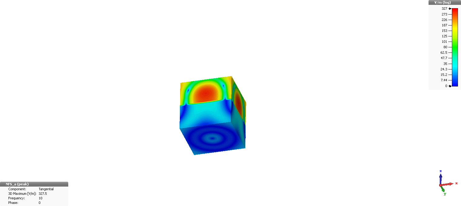 Figure 1
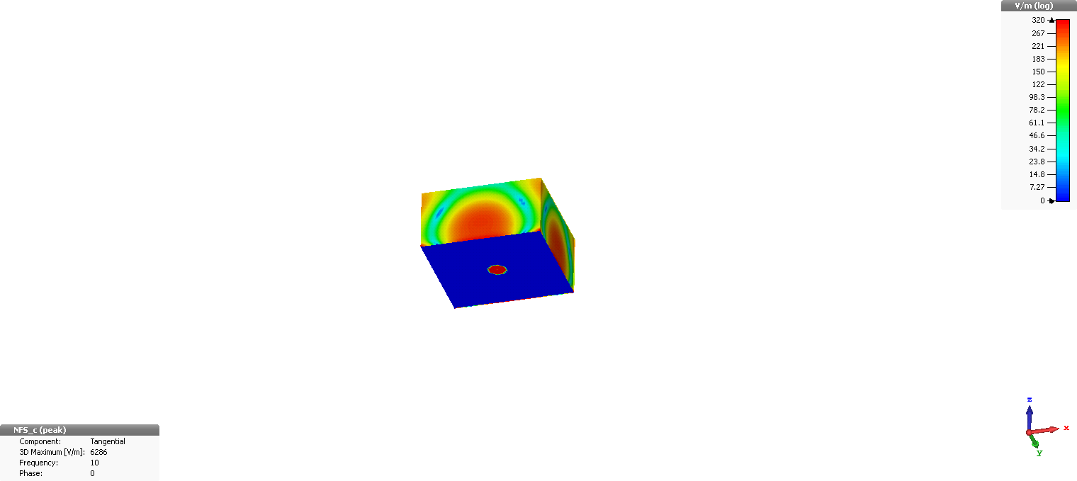 Figure 2
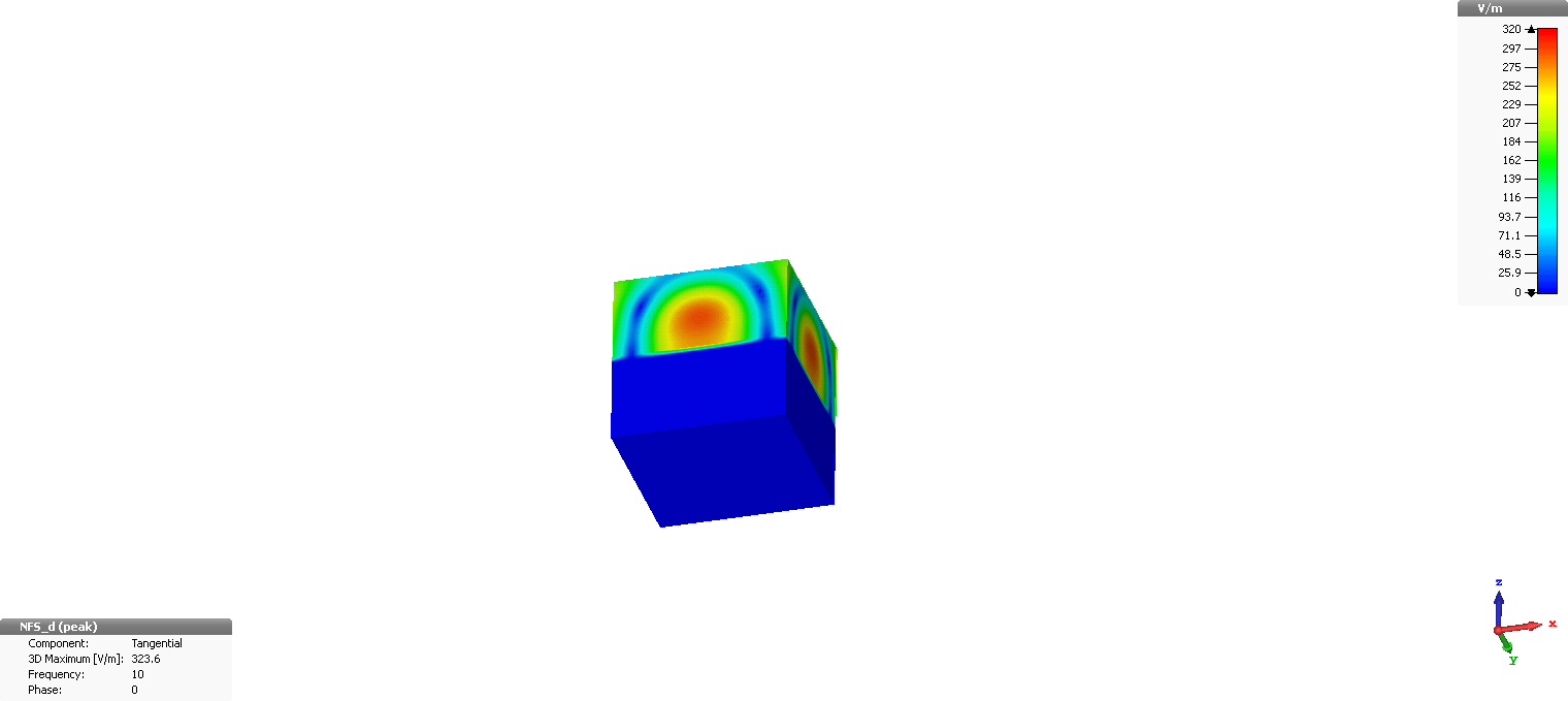 Figure 3
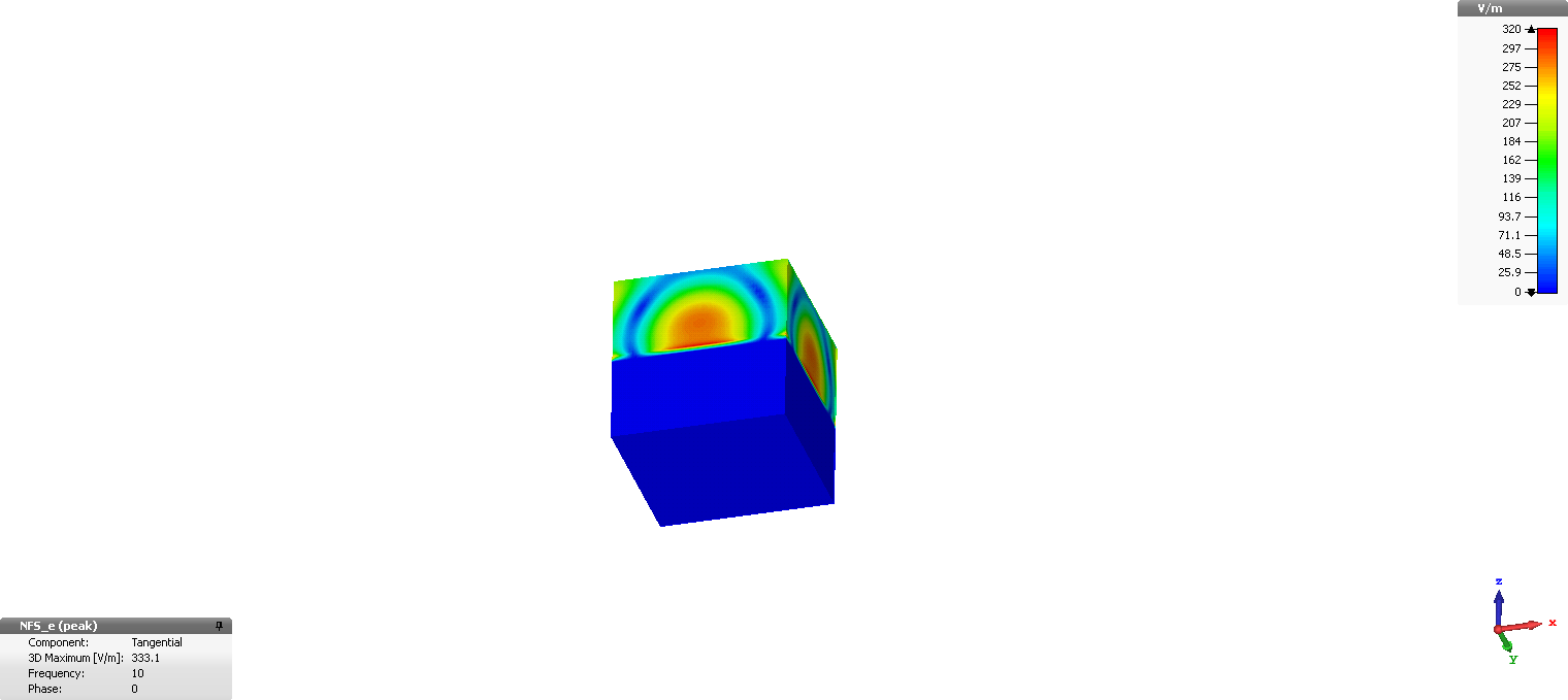 Figure 4
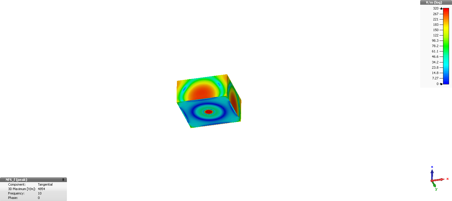 Figure 5
 Figure 6
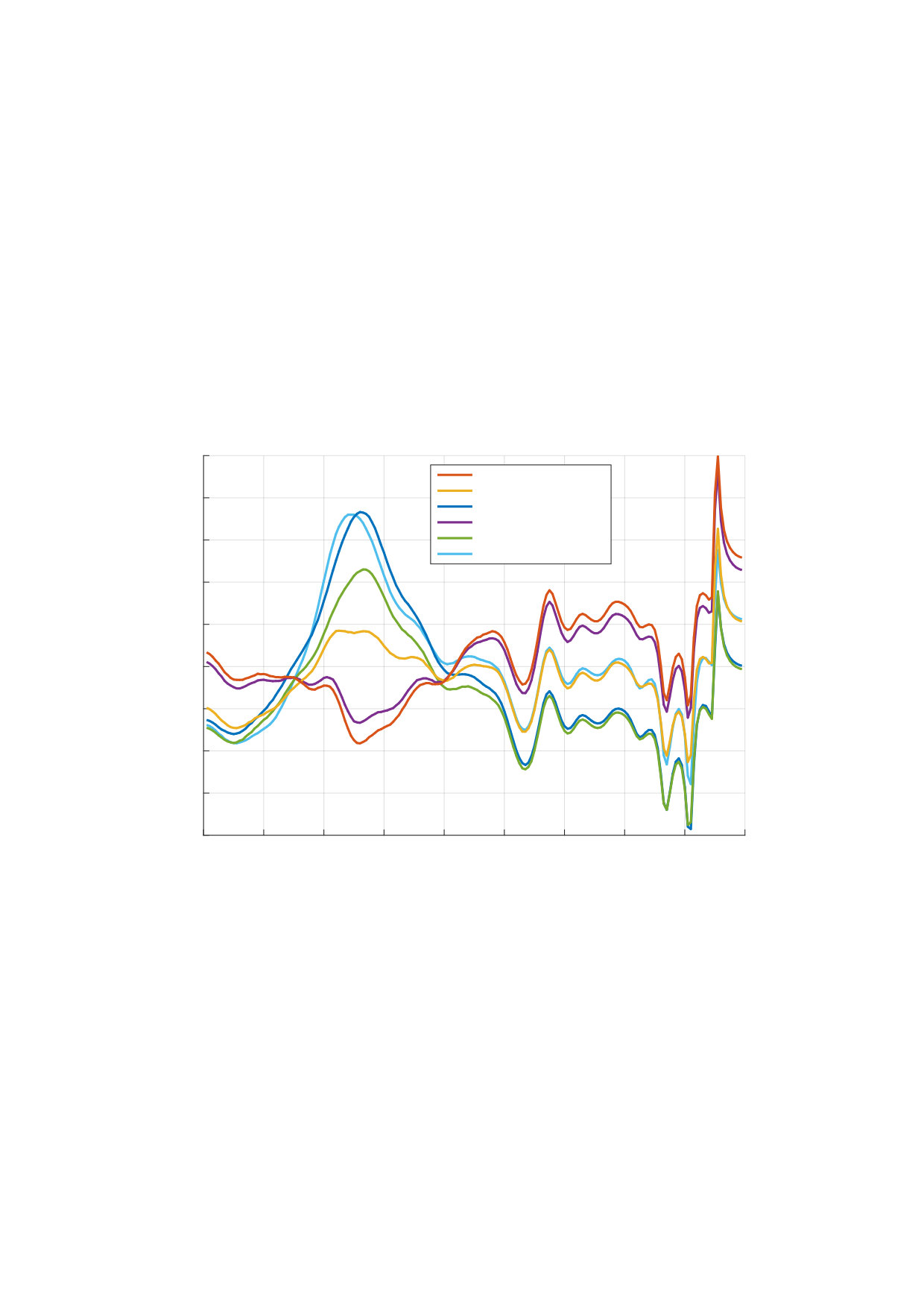 Figure 10
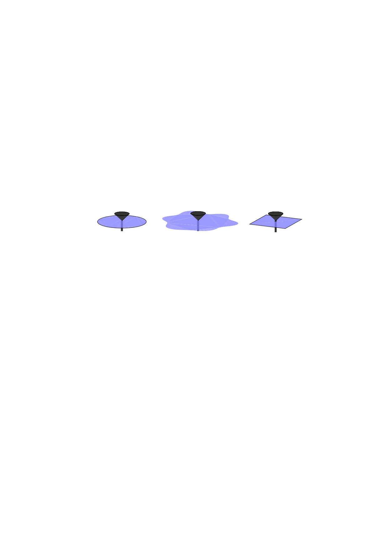 Figure 11
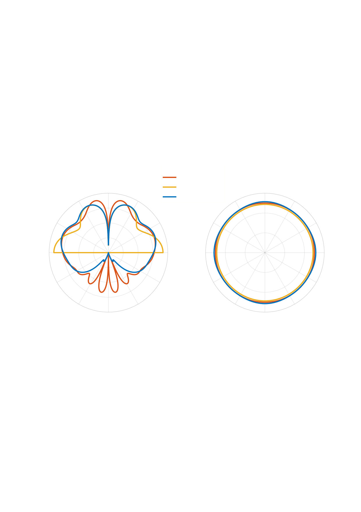 Figure 12
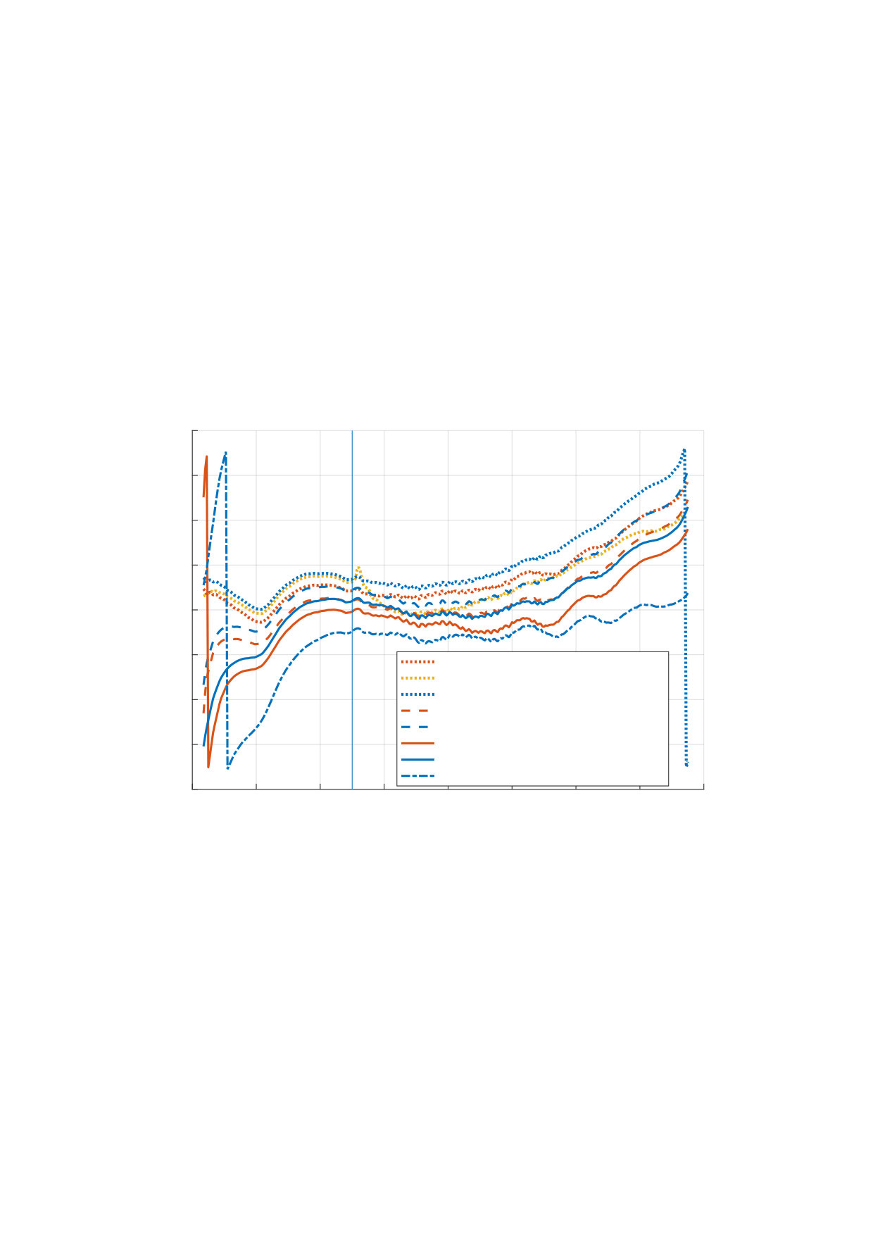 Figure 13
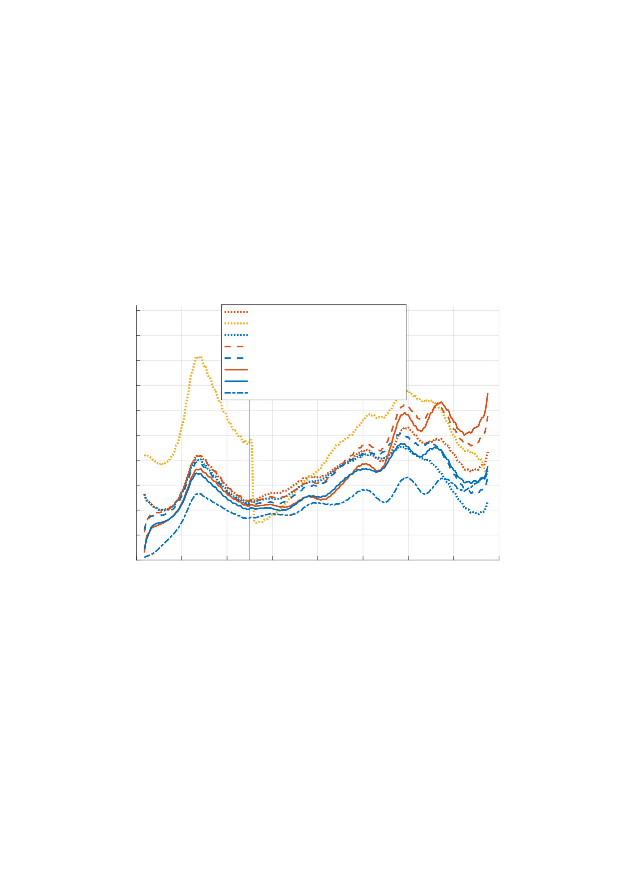 Figure 13
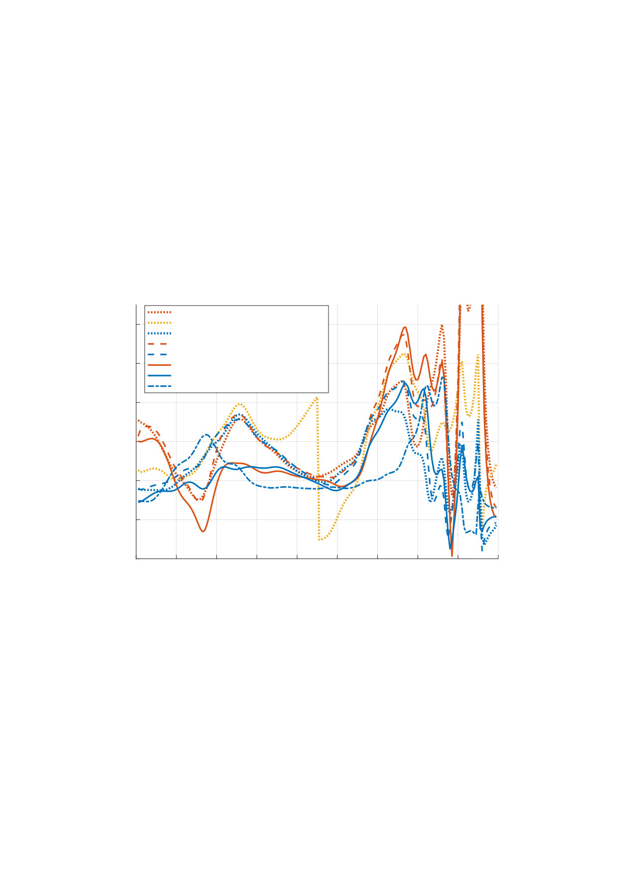 Figure 14
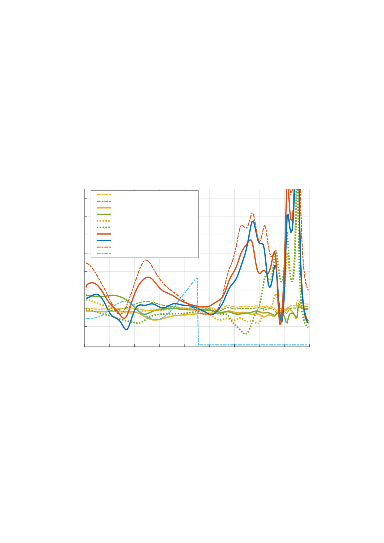 Figure 16
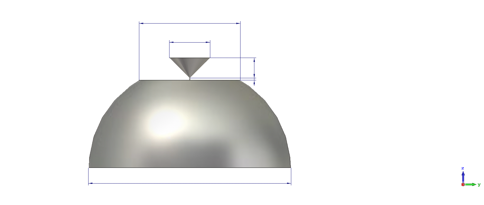 Figure 1
 Figure 2
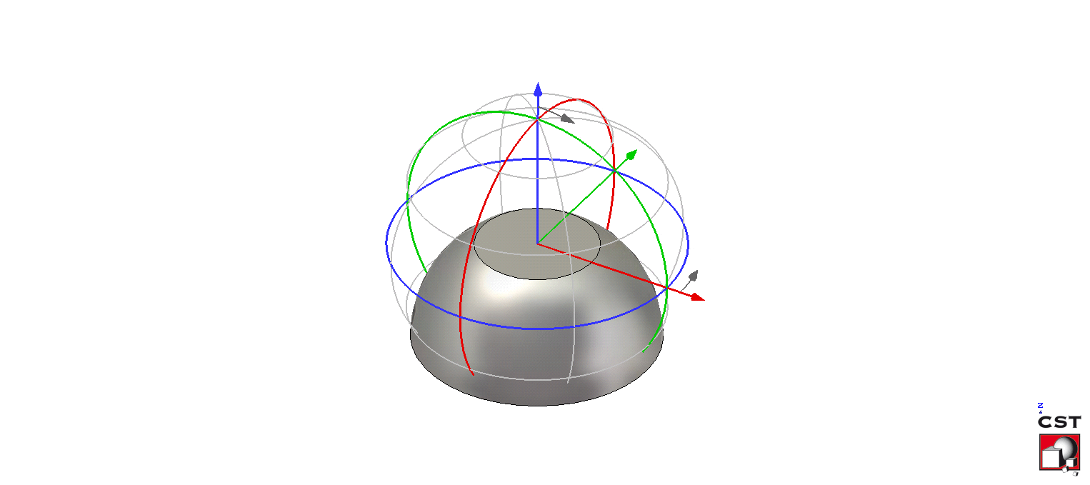 Figure 3
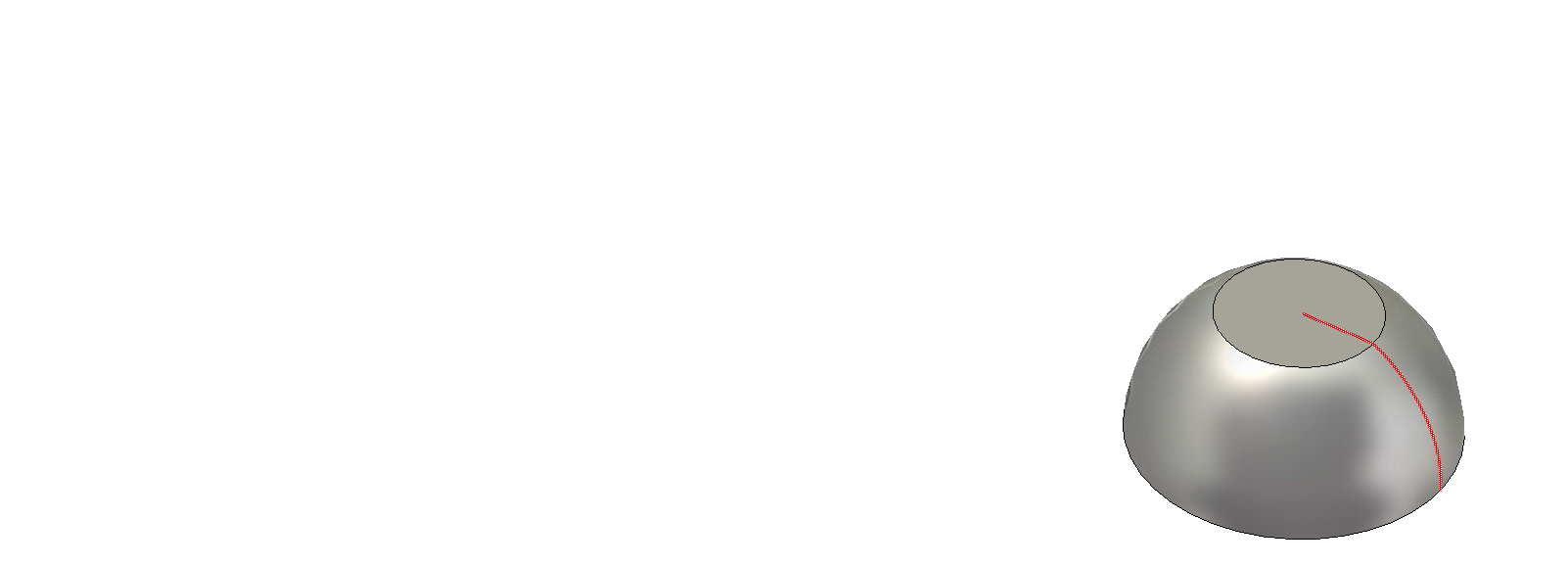 Figure 3
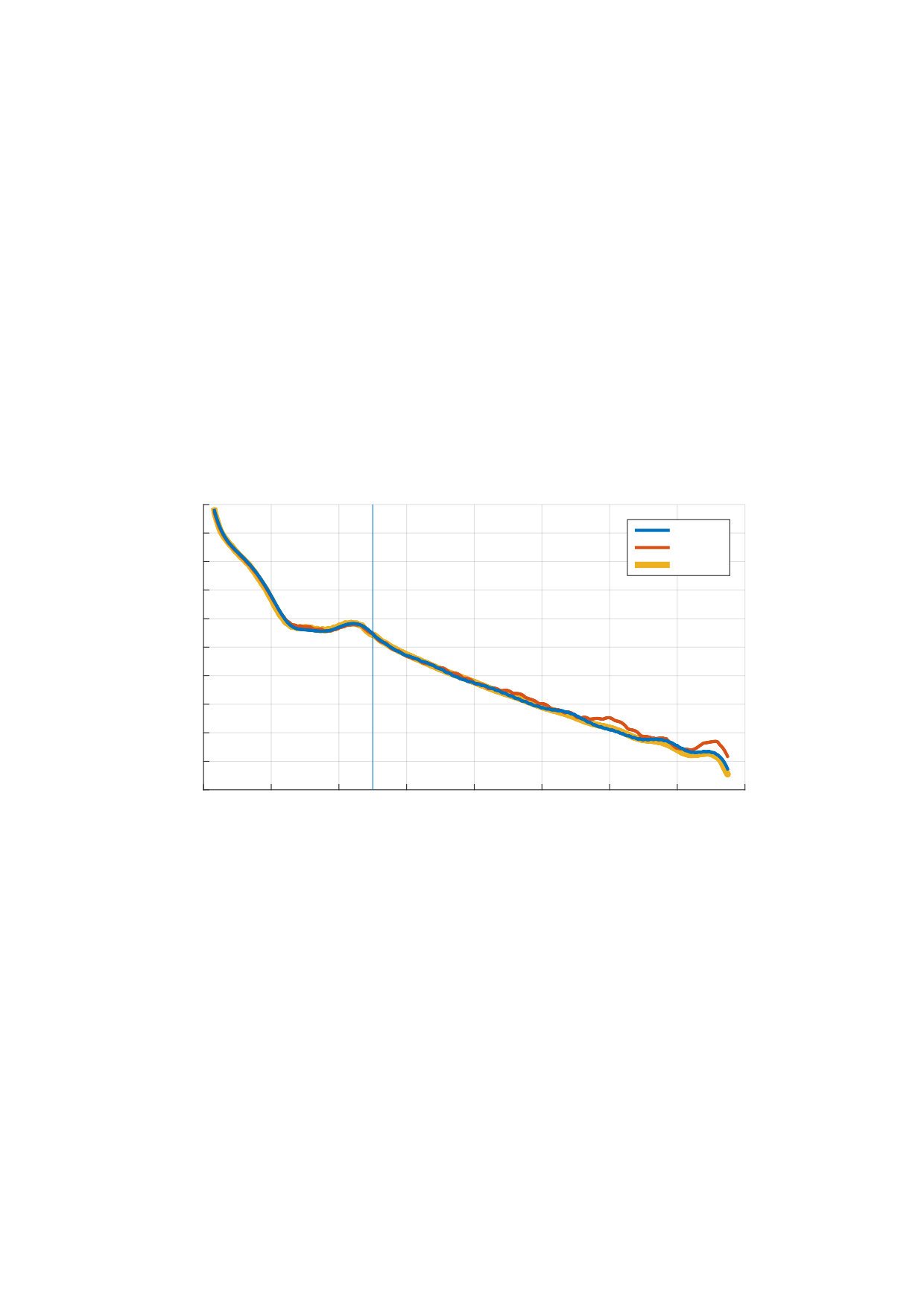 Figure 4
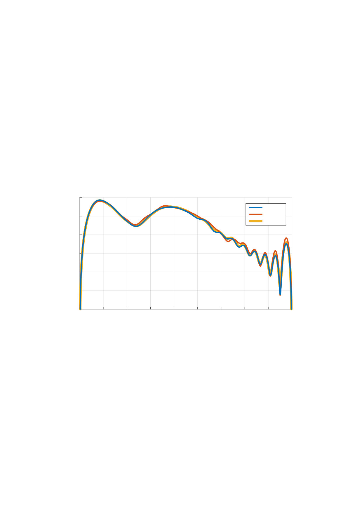 Figure 5
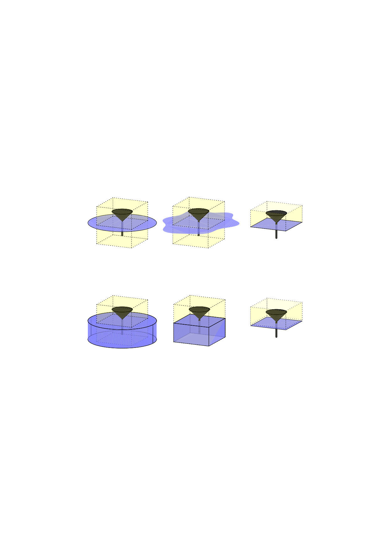 Figure 9
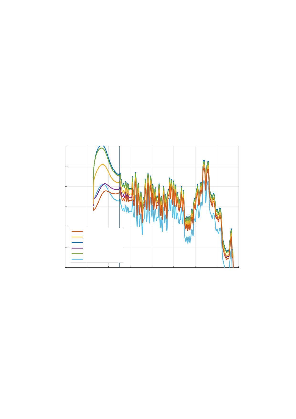 Figure 9
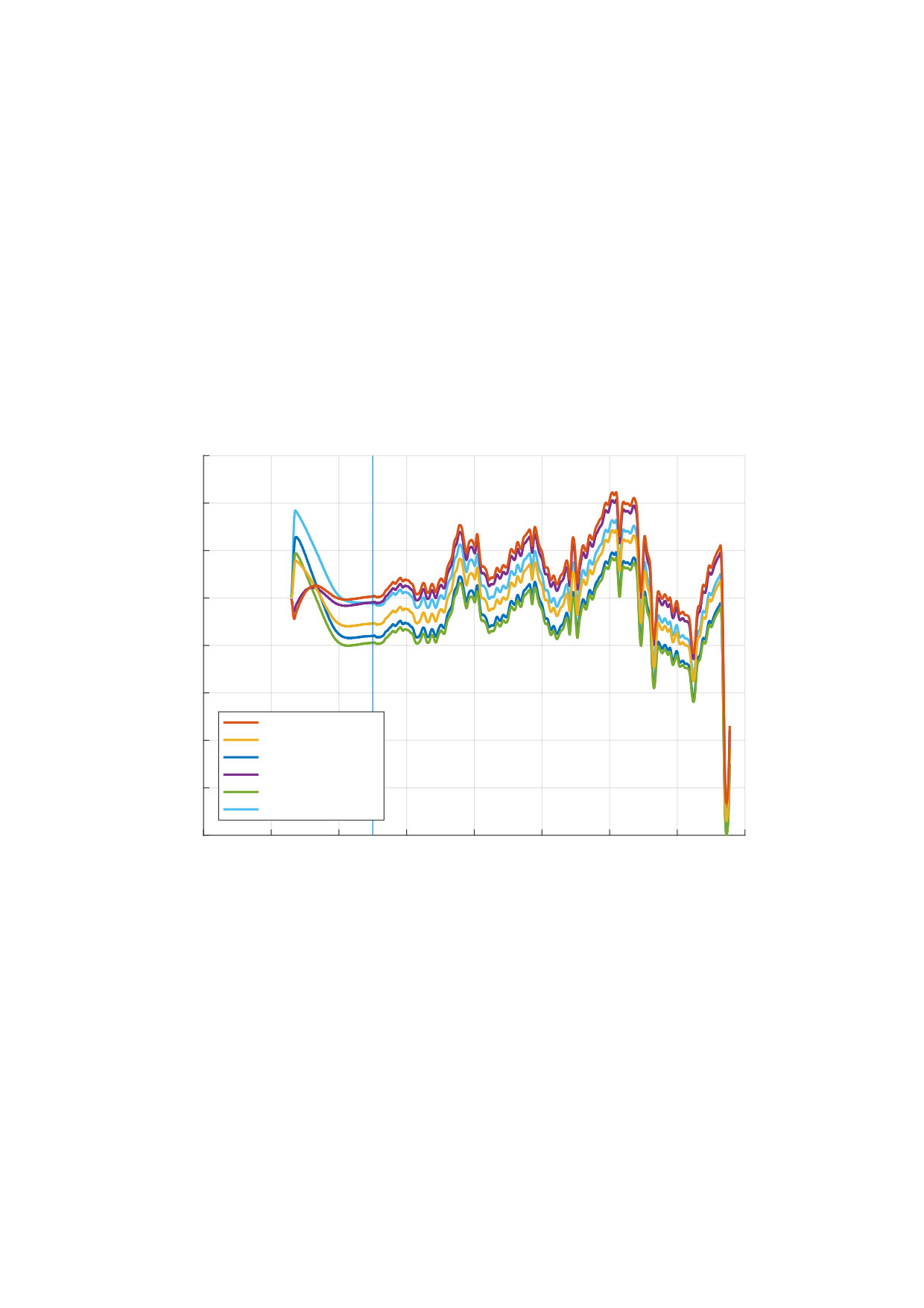 Figure 9
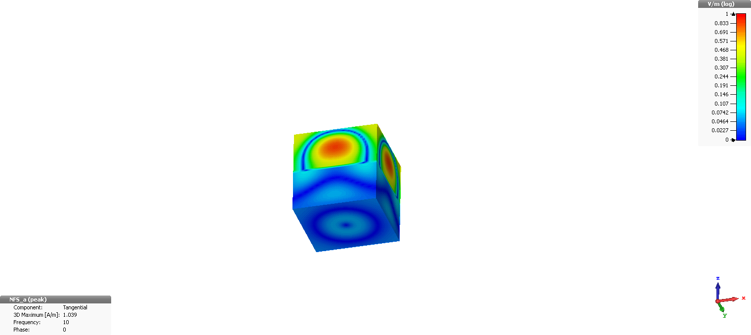 Figure 23
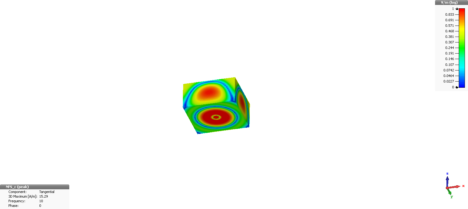 Figure 24
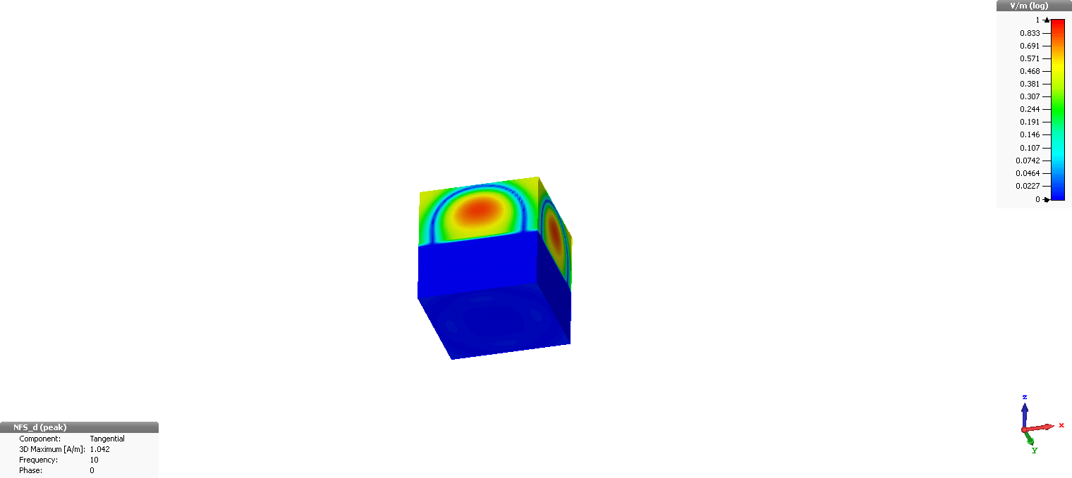 Figure 25
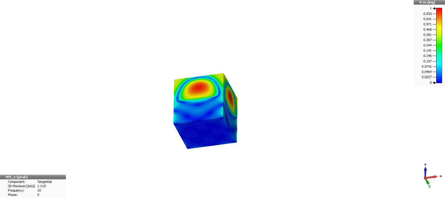 Figure 26
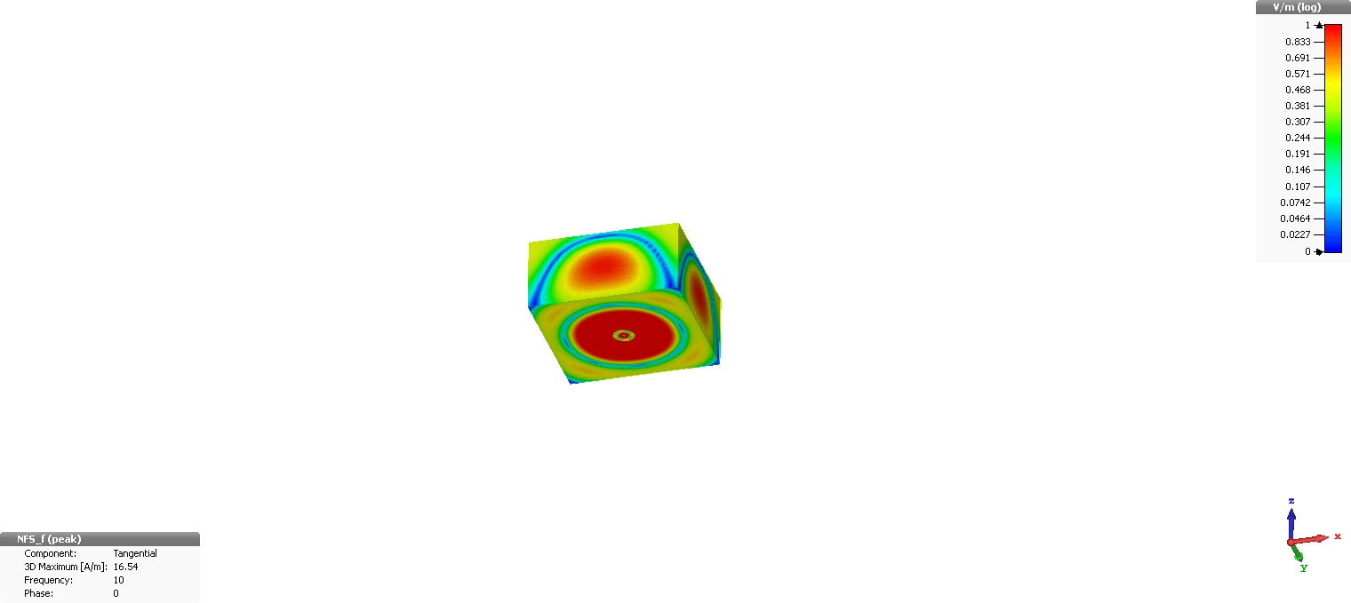 Figure 27
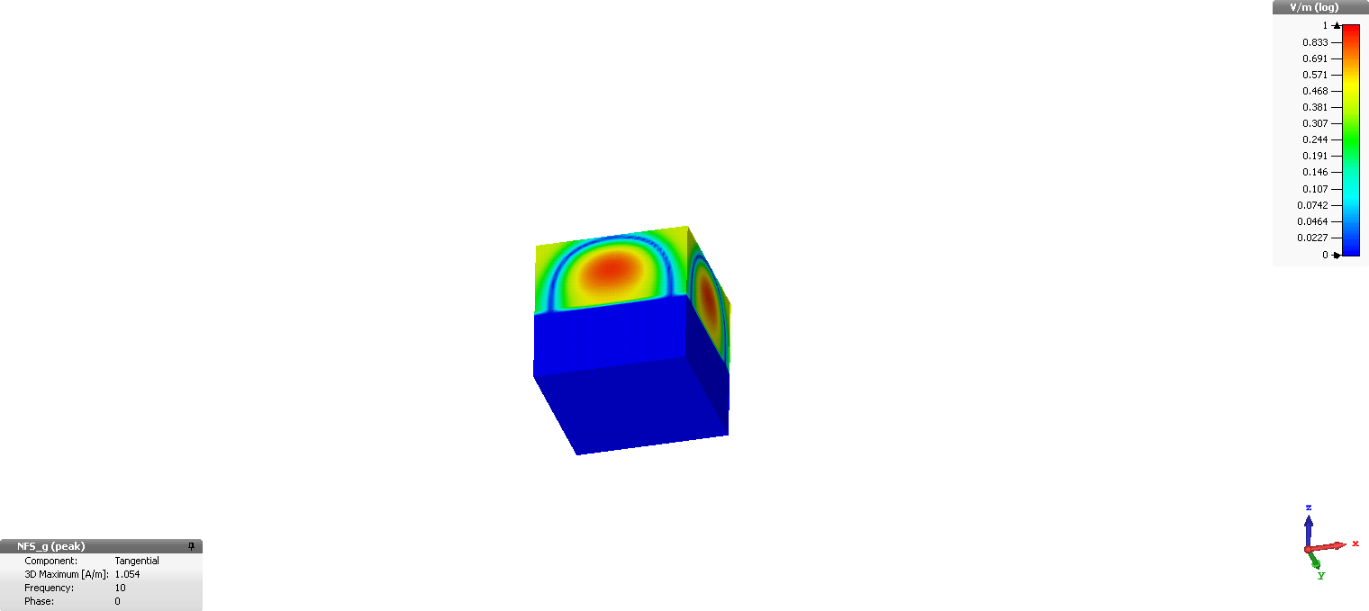 Figure 28
| Conf. | |||
|---|---|---|---|
| NFS (a) | mm | mm | mm |
| NFS (b) | mm | mm | mm |
| NFS (c) | mm | mm | , mm |
| NFS (d) | mm | mm | mm |
| NFS (e) | mm | mm | mm |
| NFS (f) | mm | mm | mm, mm |
| Configuration | RMS (linear scale) | ||
|---|---|---|---|
| , mm | , mm | , | |
| NFS (a) | % | % | |
| NFS (b) | % | % | |
| NFS (c) | % | % | |
| NFS (d) | % | % | |
| NFS (e) | % | % | |
| NFS (f) | % | % | |
| Configu- | RMS (linear scale) | ||||
|---|---|---|---|---|---|
| ration | , | , | , | , | |
| mm | mm | ||||
| FFS (a) | mm | % | % | % | |
| FFS (b) | % | % | % | ||
| FFS (c) | % | % | % | ||
| FFS (a) | mm | % | % | % | |
| FFS (b) | – | – | % | % | |
| FFS (c) | % | % | % | ||
| FFS (a) | mm | % | % | % | |
| FFS (b) | – | – | % | % | |
| FFS (c) | % | % | % | ||
| FFS (a) | mm | % | % | % | |
| FFS (b) | – | – | % | % | |
| FFS (c) | % | % | % | ||
| RMS (linear scale) | |||
| Configuration | , | ||
| FIT | MoM | SBR | |
| NFS (b) | % | % | % |
| NFS (d) | % | % | % |
| NFS (f) | % | % | % |
| FFS (a), mm | – | % | % |
| FFS (b), mm | – | % | % |
| FFS (c), mm | – | % | % |
| FFS (c), mm | – | % | % |
Peer Reviews
No public reviews on file for this paper yet. If you reviewed it on a platform where reviews are public (OpenReview, ICLR, NeurIPS, ICML), you can paste yours below so the community can read it here.
Videos
No videos yet. Explain this paper in a talk, walkthrough, or lecture? Add one.
On the Accuracy of Equivalent
Antenna Representations
Johan Malmström, Henrik Holter, and B. L. G. Jonsson J. Malmström and B. L. G. Jonsson are with the School of Electrical Engineering, KTH Royal Institute of Technology, Stockholm, Sweden.J. Malmström and H. Holter are with Saab Surveillance, Stockholm, Sweden. The work was supported by Saab Surveillance.
Abstract
The accuracy of two equivalent antenna representations, near-field sources and far-field sources, are evaluated for an antenna installed on a simplified platform in a series of case studies using different configurations of equivalent antenna representations. The accuracy is evaluated in terms of installed far-fields and surface currents on the platform. The results show large variations between configurations. The root-mean-square installed far-field error is % for the most accurate equivalent representation. When using far-field sources, the design parameters have a large influence of the achieved accuracy. There is also a varying accuracy depending on the type of numerical method used. Based on the results, some recommendations on the choice of sub-domain for the equivalent antenna representation are given. In industrial antenna applications, the accuracy in determining e.g. installed far-fields and antenna isolation on large platforms are critical. Equivalent representations can reduce the fine-detail complexity of antennas and thus give an efficient numerical descriptions to be used in large-scale simulations. The results in this paper can be used as a guideline by antenna designers or system engineers when using equivalent sources.
Index Terms:
Electromagnetic analysis, Electromagnetic modeling, Computational electromagnetics, Antenna feeds.
I Introduction
The increasing accuracy of full-wave large-scale simulation of complex electromagnetic (EM) problems has changed the industrial design-process of radio frequency (RF) systems. The construction of scaled models for measurements has widely been replaced by simulations. This work flow saves both time and money as compared to building prototypes for measurements [1]. For simulations to be trustworthy, in particular in industrial design processes, an a-priori predictable accuracy is essential.
The reason for the large interest in simulations within the electromagnetic community is that electromagnetic scattering problems are rarely possible to solve analytically. Problems involving realistic antennas are therefore usually solved numerically. For small-scale systems, a detailed model of the physical antenna serves as a good model for accurately determining associated fields, impedances, and currents with numerical methods. This is documented by e.g. the annual benchmarks given by the EurAAP working group on software [2], where different simulation methods and measurements are compared [3]. The simulations have shown an increasing agreement with measurements over the last few years [4]. For electrically large platforms, it is problematic to include models of the antenna and the complete platform in the same simulation, since the computational time and memory requirement grow with the electrical size [5].
Simulations of electrically large platforms in combination with complex antennas, can lead to extreme computational time and memory requirement. In these cases, a less complex antenna model can significantly reduce the overall complexity of the simulation. Using an equivalent representation of the antenna is one way to reduce the complexity of the antenna model. An equivalent antenna representation also opens the possibility to utilize different numerical methods in different parts of the simulation domain, sometimes referred to as a hybrid method.
On large platforms, special techniques can be used to avoid limitations of platform size from memory requirements. One commonly used technique is asymptotic methods, e.g. physical optics (PO) or geometrical optics (GO), which are high-frequency approximations. Another technique is domain decomposition that split a large simulation into several smaller sub-problems that are solved in parallel [6]. This has been used in e.g. [7, 8, 9, 10]. A drawback with domain decomposition is that the complexity is increased as compared to a full-domain simulation, since information has to be exchanged over the interface between adjacent sub-domains.
One way of decomposing a large EM problem is to analyze the antennas in isolation, and imprint the results in the platform model. In a basic domain decomposition, multiple scattering effects between structures in different domains are neglected, which implies that there is no need for iterations over the interface between adjacent sub-domains. In that case, the sub-domain with the antenna serves as an equivalent representation of the antenna, in the same way as in this work. When installing antennas on a platform, the antennas are often placed so that the scattering from the platform is minimized. Therefore, neglecting multiple scattering is often a minor approximation in antenna placement studies.
Commercial software for computational electromagnetics (CEM), see e.g. [11, 12, 13, 14], and recommendations for CEM has been thoroughly discussed in the literature see e.g. [15]. From an industrial perspective it is of major interest to get a highly accurate solution, but equally important to get a predictable accuracy. Simulation software documentation can give designers valuable rule-of-thumb recommendations about preferred equivalent model configurations, but the recommendations seldom give any information about the expected accuracy when using the equivalent representation. Unfortunately, it is not at all obvious which configuration of the equivalent antenna model that is most accurate.
Source modeling in electromagnetics has been of scientific interest for a long time, where major contributions have been made by e.g. Hallén, King and Harrington. Some of these works are reviewed in e.g. [16]. These classical works focus mainly on antenna excitations for a specific type of antenna, e.g. wire antennas. Here, we do not model the feeding, but rather use an equivalent model for the entire antenna. The two here studied equivalent representations, near-fields sources and far-field sources, are general in the sense that they can be used for any type of antenna. The underlying theories for these two representations, the equivalence principle and far-field pattern generation, are both described in literature; see e.g. [17] and the references within. They are also implemented in several commercial software, see e.g. [11, 13]. Results from using equivalent representations are described in several articles, e.g. [18, 10, 19, 20, 21], where near-field sources are used, and e.g. [22] that shows examples when using far-field sources.
The results in this paper add to the practical knowledge by examining the accuracy of equivalent antenna representations, for different parameter configurations and different numerical methods. In addition to the installed far-field, which is one of the most important characteristic of an installed antenna, we also evaluate the induced surface current on the platform, which is important in both EMC applications and in antenna placement studies [1]. The results indicates what order of magnitudes of errors that equivalent antenna models introduce. The results also serve as a guideline for an antenna designer in order to choose the most accurate configuration when using equivalent representations of antennas.
The paper consists of the following sections. Section II describe the theory used in the article and Section III the used methods and models. The results are presented in Section IV. We evaluate the accuracy of near-field sources in Section IV-B, far-field sources in Section IV-C, and their combination with different numerical methods in Section IV-D. The paper ends with a discussion and conclusions in Section V.
II Equivalence Theory
Two types of equivalent antenna representations are evaluated in this paper; near-field sources and far-field sources. Both representations are applicable to any kind of antenna or other radiating structure.
II-A Near-field Sources
The equivalence principle, introduced by Love [23] and refined by Schelkunoff [24], implies that any radiating structure can be represented by electric and magnetic surface currents on an fictitious surface enclosing the radiating structure [25]. If the material outside is homogeneous, it can be deduced that and reproduce exactly the same electric and magnetic fields outside as the original antenna, while the fields inside are zero [25, 26]. A near-field source (NFS) is a set of surface currents , on the surface , a Huygens’ surface. With the presence of a platform, the homogeneous requirement is not fulfilled and the near-field source only reproduces the original fields approximately.
The surface currents and , which we hereafter refer to as currents, are directly related to the discontinuity of the tangential electric and magnetic fields on the surface . Since the currents , produce zero fields inside the surface , the currents on can be written as [25, 27]
[TABLE]
where and are the electric and magnetic fields on and is the outward pointing normal to the surface .
It can be beneficial to use a near-field representation of an antenna instead of a model of the physical antenna. One reason is if the number of mesh cells in the model including the platform decreases. Also, it opens up for using different numerical methods when analyzing the antenna and the platform.
When an antenna is installed on a platform, the surrounding material is non-homogeneous; the platform is typically made of conducting or dielectric material that is surrounded by e.g. air or vacuum. Using a near-field source to represent the antenna in a situation when the homogeneous condition is violated introduces an error because the surface currents are not correctly described. Hence, using a near-field source under this common circumstance is an approximation. The error from this approximation is effected by the choice of sub-domain, and is evaluated in Section IV-B. The generation of a near-field source is described in Section III-B1.
II-B Far-field Sources
Antenna radiation patterns are commonly used to characterize antennas. They describes magnitude, phase and polarization of the propagating waves generated by the antenna, for directions , and a fixed distance . The far-field radiation pattern is the leading order behavior as [25].
A far-field radiation pattern can be used as an equivalent source in electromagnetic simulations. We will then refer to it as a far-field source (FFS). For reciprocal antennas, it also describes the receiving characteristics of the antenna. The far-field source is characterized by its far-field radiation pattern imposed as an infinitesimally small source at a given position. This position together with the approximation of the platform when generating the far-field source, are the design parameters for far-field sources. Their impact on the accuracy of the solution is non-trivial, and is examined in Section IV-C.
Far-field sources are, compared to near-field sources, more a primitive representation, and are not expected to perform as good. On the contrary, they provide very efficient representations in numerical methods, from an implementation point of view. The error introduced by the far-field approximation is small when the far-field source is far from surrounding structure, e.g. a horn antenna feeding a parabolic reflector, see e.g. [28]. However, far-field sources have be used also near structures, see e.g. [22].
Multipole expansion is a procedure to increase the accuracy of a far-field approximation close to the source point, i.e. in the near field region [27]. However, with a far-field source installed on a platform, multipole expansion cannot be used, since it requires that there is no charge or current carrying structure within a certain distance from the center point of the expansion [27]. Multipole expansion is therefore not further considered in this paper.
Using a far-field source, its emitted radiation will locally be a plane wave, irrespective of the true distance between the far-field source and an evaluation point. A far-field source can be used e.g. in an integral equation formulation, where the point source is used as a field source within the computation domain. Implementation details of the point-shaped far-field source depend on the type of numerical method used, see e.g. [29, 30, 5] for general discussions. The generation of a far-field source is described in Section III-B2.
III Methods
We use a series of case studies to investigate the accuracy of equivalent antenna representations for different configurations. For electromagnetic problems, where analytic solutions can rarely be found, the case study is an effective tool to compare configurations. The aim is to determine how equivalent antenna representations affect the accuracy of fields and currents in the presence of a platform and to obtain an understanding of the relation between configuration of the equivalent antenna representation and accuracy.
III-A Geometrical Model
We choose here a platform geometry and an antenna .
The platform geometry should have a simple and well defined shape, but still retaining platform specific features for installed antennas. The chosen platform geometry is depicted in Fig. 1. The geometry is a cut mm diameter half-sphere, where the diameter of the cut top is mm. It is perfectly electrically conducting (PEC). The geometry is of electrically size about at 10 GHz and has the following platform like properties:
- •
Finite support of surface currents,
- •
weak back-scattering from its edges to the antenna,
- •
radiating creeping waves on the curved surface.
The antenna chosen for this case-study is a mono-cone antenna, also depicted in Fig. 1, with mm top radius and mm height. The mono-cone antenna is mounted centrally on the flat top surface of the main geometry with a mm feed gap. It is fed with a wave-guide port via a mm long coaxial cable. A mono-cone antenna has an isolated far-field radiation pattern similar to a mono-pole but is more wideband.
We are interested in determining fields and currents in the domain on and outside the geometries . Since the main geometry and the mono-cone antenna are both rotational symmetric, it implies that fields and currents must have the same rotational symmetry. It is hence sufficient to evaluate symmetric quantities on a plane and a fixed azimuth .
III-B Calculation Domains
The following domain definitions, as in Fig. 2, are used:
- •
The domain that contain the platform geometry and the antenna .
- •
A sub-domain that contain the antenna and a selected part of the platform. As the equivalent source is intended to improve calculation time and memory use, the sub-domain should be much smaller than the domain .
- •
A Huygens’ surface , i.e. a fictive surface enclosing the antenna. The Huygens’ surface is completely included in the sub-domain .
In a platform specific problem, e.g. with aircraft or ships, the domain is often electrically very large. However, in this work, we use a comparatively small domain . This allows us to obtain a highly accurate reference solution for the fields and currents from the installed antenna, which is subsequently used as our benchmark. The equivalent sources can be used on electrically large structures as well, so the methods and observations are applicable to antennas on e.g. ships or aircraft.
An antenna induces currents on surrounding structures. Such currents also contribute to the equivalent source. By using the small domain to determine the equivalent sources, we implicitly ignore all currents outside . The larger the sub-domain is, the smaller the error will be, but the computational cost to determine the equivalent source increases with growing size of .
III-B1 Work Flow for Using an Equivalent Near-field Source
- •
In the sub-domain ; Calculate the tangential electric and magnetic fields, and , on the surface generated by the antenna, see Fig. 2(b).
- •
In the domain ; Remove the model of the physical antenna111Instead of removing the antenna model, it can be replaced by a simplified model to include some of the multiple scattering effects that the model of the physical antenna model would give. and imprint the equivalent currents and on , see Fig. 2(c).
- •
Solve the problem in the domain using , as equivalent sources.
We use a rectangular box as surface for the equivalent currents that define the near-fields source.
III-B2 Work Flow for Using an Equivalent Far-field Source
- •
In the sub-domain ; Calculate the far-field radiation pattern generated by the antenna, see Fig. 2(b). This is the equivalent far-field source.
- •
Choose a height over the main geometry where the far-field source is imprinted.
- •
In the domain ; Remove the model of the physical antenna and solve the problem using the far-field source, see Fig. 2(d).
The procedures described above in III-B1–III-B2 is general and applies to any kind of structure, not only the platform and the antenna used in this case study.
III-C Evaluation
The results in e.g. [2, 3, 4] indicate that full-wave simulation results can be used as a benchmark of antenna behavior. We evaluate the electric current and the installed far-field pattern by comparing simulations with equivalent antenna representations against an accurate reference solution using the model of the physical antenna.
In order to get reliable estimates of the accuracy, it is crucial to have a highly accurate reference solution. We verify that the solution is accurate by solving the reference case with three different numerical methods; Finite integration technique (FIT), Method of moments (MoM), Finite element method (FEM), see e.g. [31, 32, 5].
When comparing results from simulations, one must keep in mind that different settings, e.g. the mesh, will affect the results. The results in this paper are from simulations where the solver settings are not the main limiting factor for the accuracy, but rather the representation of the antenna.
Two of the most important antenna quantities are installed far-field patterns and isolation between antennas [1]. The installed far-field patterns are of large importance when determining the functionality of a radio frequency (RF) system, which is determined e.g. by the coverage for a sensor installed on a vehicle. There can be a large difference between an antennas isolated radiation pattern, which is the radiation pattern for the antenna in free space, and its installed radiation pattern, which is the radiation pattern when installed on a platform. Hence, as is well known, antennas must be analyzed within their complete environment [33]. The isolation between antennas is related to the risk for interference between the antennas. It is an important quantity in antenna placement studies [1]. The isolation between antennas are mainly determined by direct propagating waves and surface currents, see e.g. [34]. The accuracy of surface currents is thus an important contribution to the accuracy of isolation between antennas, in particular for antennas without line-of-sight.
The following quantities are used for evaluating the accuracy of the results using the equivalent sources:
- •
The electric current along the red curve in Fig. 3(b).
- •
The installed far-field for all inclination angles and a fixed azimuth .
We use (1) to evaluate the electrical current based on the magnetic field . The magnetic field can be separated into components parallel and orthogonal to the azimuthal unit vector ,
[TABLE]
The propagating component is dominant outside the reactive region, so that we can make the approximation . With this approximation, the electric current can be calculated as
[TABLE]
The rotational symmetry implies that , where is the outward pointing tangent unit vector along the curve in Fig. 3(b). The tangential current along the curve is
[TABLE]
We denote the complex tangential current from the references solution and when using an equivalent source . The scalar is the arc length along the curve in Fig. 3(b). We define the relative magnitude error and the phase error of the complex current as
[TABLE]
where denotes the argument of a complex number.
The installed electric far-field is also separated into its components parallel and orthogonal to the azimuthal unit vector , so that
[TABLE]
Due to symmetry, . On large distances from the antenna, the radial component vanishes, so that
[TABLE]
We denote the complex electric far-field component from the references solution , and when using an equivalent source . From the electric far-fields and , we can evaluate both the magnitude error and the phase error. However, in this paper we only evaluate the magnitude error of the installed far-field, which is the most commonly used quantity to classify installed antennas. We define the relative magnitude error as
[TABLE]
When calculating the current , by using (6), we evaluate a small distance above the surface. The reason for this is numerical stability. The field will be zero inside the PEC structure, and by setting we assure that the evaluation points are not inside the structure. We use mm. By evaluating the far-field component we will be able to see systematic errors, which would be hidden in the normalization if e.g. the directivity was evaluated.
Note that it is the field components and in their respective regions that are used as inputs to the benchmarks in (7)–(8) and (12). Hence, the approximations in (6) and (11) do not affect the accuracy of the benchmark222For a rotational symmetric problem, as in this case, the expressions (6) and (11) are exact.. The introduced notation, , and , is motivated by the physical relevance of these quantities.
III-D Solvers and Simulation Settings
To evaluate the accuracy of the equivalent sources we need a reference case. We use a full wave solution of the detailed antenna model in Fig. 1 as the reference. It is thus crucial that the reference solution is reliable. We here utilize two observations: that commercial solvers have high accuracy [3] and that different numerical methods yield similar solutions.
The equivalent sources are generated using FIT. In the evaluation of the equivalent sources, we examine their robustness, with respect to design parameters, by using them as excitations and solve in the full domain using FIT or MoM, as well as the asymptotic method Shooting-Bouncing-Rays (SBR).
All simulations are performed at GHz using CST Microwave Studio (MWS) [11]. The frequency is chosen so that fields in the domain can be calculated with full-wave methods on a desktop computer. The size of the domains and is set so that they contain the structure of interest and of space on each side.
IV Results
IV-A The Reference Solution
To examine the variability of the reference results, we use three numerical methods, FIT, MoM and FEM, applied to the model in Fig 1 with a model of the physical antenna.
The magnitude of the tangential electrical current, , along the line in Fig. 3(b), is depicted in Fig. 4. The currents calculated with different methods agree well, with a relative RMS difference between FIT and MoM currents of %. The difference between FIT and FEM is % and between MoM and FEM it is %.
The installed far-field magnitude is depicted in Fig. 5 for the azimuthal direction and . Again, the results from the numerical methods agree well, with a relative RMS difference between the far-fields calculated with FIT and MoM of %. The difference between FIT and FEM is % and between MoM and FEM it is %.
The agreement of the results from the different numerical methods indicate that the reference solutions are accurate. We see in Fig. 4 that the solutions using MoM and FIT conform best with the expected exponential decay of the current on the curved surface. Of these two solutions, with good mutual agreement, the FIT solution is chosen as the reference, since FIT is the native solver in CST MWS.
We can relate some of the properties seen in Fig. 4–5 to the platform. The slope of surface current in Fig. 4 for mm depends on the curvature of the sphere. The double beam at , , and the local minimum between, of the installed far-field in Fig. 5 is an effect of the flat top surface of the platform. A smaller radius of the flat top would lift the beams, i.e. decrease the inclination angle . The oscillations for in Fig. 5 are caused by reflections in the bottom edge of the platform .
IV-B Results for the Near-field Source Configuration
The realization of near-field sources depend on the choice of the sub-domain and the placement of the surface , see Fig. 2, but also on the choice of ground-plane geometry. The aim here is to evaluate the freedom of choice with respect to these geometrical parameters. We consider six different configurations of surfaces and ground planes, as defined in Fig. 6, with dimensions given in Table I. The configurations evaluated are motivated briefly below.
Configuration (a) is generated with a thin sheet PEC plate and has non-zero currents also on the lower half of , as can be seen in Fig. 7(a) and Fig. 8(a). The same applies to (e), because coincide with the PEC boundary. The infinite ground plane in (b) is essentially estimating the whole platform as a ground plane, whereas (a) and (d) account for the local geometry of the platform. The diameter of the circular PEC plate for the configurations (a) and (d) is mm () and corresponds to the flat top of the platform , see Fig. 1.
Configuration (b) uses an infinite ground-plane. Hence, there will be no discontinuities in the surface currents on the ground plane. In configurations (d) and (e) the ground-plane is solid, resulting in a edge at radius mm on the ground plane. In the other configurations, (a), (c), and (f), the ground planes are thin sheets, resulting in sharp edges.
One of the key features in (a) and (d) is that they capture a larger part of the platform geometry as compared to the other configurations. Configurations (c), (e), (f) all take a ground plane with a side length mm () that correspond to the horizontal size of the equivalent surface . The effect caused by the currents on the ground plane can be observed by comparing (c) and (f), since the surface coincide with the ground plane in (c) while it is mm above the ground plane in (f). Note that the square ground plane in configurations (c), (e), (f) does not conform to the azimuthal symmetry of the original problem. However, the field solutions corresponding to configurations (c) and (e) show less asymmetry than (f), as can be seen in Fig. 8, possibly due to the effects of the ground plane that coincide with in (c) and (e), but not in (f). An advantage of setting the ground-plane size equal to the size of the surface , as in (c), (e), and (f), is that the sub-domain is minimal, leading to shorter simulation times.
The work flow described in Section III-B1 is followed when generating and using the near-field sources. Since the reference solution was solved with FIT, we use FIT again to solve the problem with the near-field sources imprinted in the platform model.
The resulting near-field source representations of the antenna are depicted in Fig. 7–8, for each of the configurations used. The strong fields on the bottom surface of (c) and (f) is due to the coaxial feed cable that penetrates the surface .
The accuracy is evaluated by the tangential current errors and , according to (7) and (8). They are presented in Table II as RMS errors and depicted in Fig. 9 for the interval mm, i.e. outside the equivalent surface . The installed far-field errors , according to (12), are depicted in Fig. 10 and the RMS errors for are listed in Table II.
The best behavior in terms of is given by configurations (d) and (a) with % and % relative error, respectively, whereas (c), (e), (f) are the worst, with about twice as large relative errors as (a) and (d). The correct local geometry of the ground-planes in (a) and (d) is important for the accuracy of the surface currents.
For the installed far-field in Fig. 10, we see that the variation is smaller between the different configurations, as compared to the current error in Fig. 9. This is expected due to the smoothing effect for far-fields. The smallest RMS error are for (b) with % and (d) with %, which are comparable with the variations of the reference solutions on %. In Fig. 10 the difference between configuration is particularly large in the region , motivating a closer study. The max-norm deviations in this region range from with (b) to with (c) and (f). We see that the edge of the ground-plane seems to play an important role for the accuracy in this region, where (b) performs best (no discontinuity), and the configuration with a square thin sheet ground-plane, (c) and (f), give the least accurate results. Comparing (a) and (d), we see that (d) with a solid ground-plane ( edge) is more accurate than (a) with a thin ground-plane (sharp edge). We see the same pattern when comparing (c) with (e); the solid ground-plane performs better than the thin sheet ground-plane with a sharp edge. The size of the ground plane also plays a role. A small ground plane gives a lifting effect of the pattern from the horizontal plane (as discussed in Sec. IV-A). The large errors for (c), (e), (f) is partly caused by this effect, where the beam maximum is shifted from to . The computationally simple configuration (b) with an infinite ground-plane gives accurate results, especially for the installed far-fields.
The expected higher sensitivity of the currents as compared with the far-field is clearly observed with a difference of a factor of about two for RMS errors. Compared with the estimated RMS uncertainty in the reference solutions in Section IV-A (% for the current magnitude and % for the installed far-field magnitudes), we see in Table II that the near-field sources increase the current magnitude uncertainty with a factor of – and the far-field magnitude uncertainty with a factor of – .
To conclude this section, we note that the RMS errors of the currents, is about % for the best case (see Table II), with max-norm deviations up to % for mm, rising up to % close to the bottom platform edge at mm (see Fig. 9). Similarly, the phase has about RMS error for the best configurations (see Table II), with max-norm deviation up to (see Fig. 9). For the installed far-fields, we note that the RMS errors are about % for the best cases, with corresponding max-norm deviations up to % over . We note that the RMS errors of the far-field vary with a factor of two between the most and least accurate configurations.
IV-C Results for Far-field Source Configuration
When generating the far-field sources, we consider three configurations, all defined in Fig. 11. From these configurations, we use FIT to calculate their far-field patterns. The results, which are used as far-field sources, are depicted in Fig. 12(a) for the vertical cut and Fig. 12(b) for the horizontal cut . The inclination is depicted since the three far-field patterns have similar magnitude making it easy to compare the curves and identify asymmetries. Note that configuration (b), with an infinite ground plane, results in a far-field pattern that is identical to zero in the lower hemisphere, . Configuration (c) will not preserve the symmetry in of the original problem, but the effect is small, as can be seen in Fig. 12(b).
The work flow described in Section III-B2 is used for generating and using the far-field sources. Because of the rotational symmetry of the platform geometry , the far-field source is placed on the symmetry axis , . In contrast, the position on the vertical axis is not trivial. Compared to e.g. a geometrical theory of diffraction (GTD) formulation [35], the source, in that case a dipole moment, can be placed both on the conducting surface or above it. We investigate four cases of the design parameter mm, i.e. the distance above the flat platform top, see Fig. 2. The resulting problem is solved with MoM, since FIT in CST Microwave Studio [11] cannot handle far-field sources.
The accuracy of the far-field sources are evaluated with the current errors and , according to (7) and (8). These errors are depicted in Fig. 13 and listed as RMS errors in Table III for the investigated configurations. The far-field errors , according to (12), are depicted in Fig. 14.
The ground plane in (c) is smaller than the flat surface of . Despite that, as depicted in Fig. 12, far-field source (c) radiates less in the lower hemisphere, as compared with (a) and (b). We note in Table III that the far-field error is smallest with (c), especially for . This is somewhat surprising, since (a) captures the local geometry of the platform better. However, the asymmetry of (c) makes it less attractive to use.
If (b) is installed on a height mm, there are no fields impinging on the platform, resulting in zero currents on the platform and also zero field for (which is the reason for the omitted numbers in Table III). Hence, when generating a far-field source using an infinite ground plane, the resulting far-field source should be installed on the platform surface, i.e. . For the other far-field sources, i.e. (a) and (c), it is hard to give any recommendations for the value of .
Compared with the estimated RMS uncertainty in the reference solutions in Section IV-A (% for the current magnitude and % for the installed far-field magnitudes), we see in Table III that the far-field sources increase the current magnitude uncertainty by a factor of – and the far-field magnitude uncertainty by a factor of – (for ).
Since the near-field behavior is not captured with far-field sources, it is expected that the surface currents are inaccurate. It is notable, however, that also the installed far-fields depicted in Fig. 14 are more inaccurate, as compared to using NFS. It is also notable that the placement of the far-field source has such a strong impact, see Fig. 13–14. Its influence is in same order of magnitude as the choice of configuration.
IV-D Results on the Impact of the Numerical Method
The above discussed results evaluate the accuracy of two different types of equivalent antenna representations. To determine how the estimated accuracy depends on the choice of numerical method, we use the best near-field configurations, see Fig. 10, and the best far-field source, see Fig. 14, with different numerical methods. For near-field sources, we compare the accuracy of FIT with the accuracy of MoM and SBR. For the far-field sources we compare the accuracy of MoM with SBR. We do not consider FIT for far-field sources since it is not implemented in the current version of CST.
We use a subset of the equivalent sources from previous sections; three near-field sources; NFS (b) with best , NFS (d) with best , and NFS (f) with best , and three far-field sources, FFS (a) mm with best , FFS (c) mm with best , and FFS (c) mm with best . The relative installed far-field errors , defined in (12), from these equivalent sources are calculated with different numerical methods, FIT, MoM, and SBR. The resulting errors are depicted in Fig. 15 and also listed as RMS errors in Table IV.
We see in Table IV that, when using near-field sources, FIT performs significantly better than MoM and SBR. On average, RMS errors are times higher with MoM and times higher with SBR, as compared with FIT.
When using far-field sources, MoM gives more accurate results than SBR, as seen in Table IV. None of the numerical methods give accurate results for with far-field sources, see Fig. 15. With the combination of FFS (b), mm and SBR, there are no fields impinging on the platform, resulting in a zero field for . In Fig. 15, it is clear that the near-field sources are an order of magnitude more accurate than the far-field sources. Similar effects are observed in the currents as seen by comparing Table II with Table III.
V Discussion and Conclusions
Electromagnetic simulations of antennas installed on large platforms are challenging problems. The often complex antenna in combination with an electrically large platform leads to very high memory requirements and long simulation times. One way to reduce the complexity is to represent the antenna with an equivalent model that is more effective to use in simulations.
This paper presents one of the first accuracy studies of equivalent sources on platforms. The presented work aims toward estimating the accuracy when using two different equivalent representations of antennas, near-field sources and far-field sources, installed on a simplified platform. Several different configurations has been considered, with respect to the approximation of the platform and geometrical parameters associated with the generation of the equivalent sources. The determined deviation from the reference solution are presented for each of the examined configuration of the equivalent sources. The results can be used as recommendations for antenna designers and engineers to choose the most accurate equivalent source configuration.
In agreement with previous knowledge, near-field sources perform significantly better than far-field sources for all configurations considered. The results with near-field sources are of the right order of magnitude for all configurations evaluated, while the errors with far-field sources are unexpectedly large for some configurations.
We observe that near-field sources, in the presence of a platform, were comparably robust, with respect to location and size of the equivalent surface. The resulting RMS accuracies of the best cases evaluated are about % and for the surface current magnitude and phase, respectively, and about % for the installed far-field magnitude.
The accuracy of the far-field sources with respect to surface current phase is rather low. In our opinion, far-field sources should not be used when current phase information is required. In the best case investigated, the installed far-field RMS error on the magnitude is about % and for the current %. The installed height above the platform of the far-field source has a strong effect on the accuracy, which introduce an uncertainty in the use of far-field sources. One should bear in mind that a far-field source, even though less accurate compared to a near-field source, is an efficient representation to use in numerical calculations. If the expected accuracy is within requirements, far-field sources can still be an attractive representation.
For the implementations in CST Microwave Studio, the most accurate results in these case-studies are obtained when using near-field sources in combination with the full-wave solver FIT. With far-field sources, the accuracy is similar with MoM and SBR for directions within line-of-sight, while MoM performs better for non-line-of-sight directions.
The reference list from the paper itself. Each links out to its DOI / PubMed record.
- 1[1] T. M. Macnamara, Introduction to Antenna Placement and Installation . John Wiley & Sons, 2010.
- 2[2] Eur AAP, “Eur AAP Working Group on Software (WG 4),” 2016.
- 3[3] G. A. E. Vandenbosch and F. Mioc, “Bridging the simulations-measurements gap: State-of-the-art,” in 2016 10th Eur. Conf. Antennas Propag. , 2016.
- 4[4] G. A. E. Vandenbosch, “Measurements and Simulations of the GSM Antenna,” in 2016 10th Eur. Conf. Antennas Propag. , Davos, 2016.
- 5[5] T. Rylander, P. Ingelström, and A. Bondeson, Computational Electromagnetics , 2nd ed. Springer-Verlag New York, 2013, vol. 51.
- 6[6] A. Toselli and O. Widlund, Domain Decomposition Methods – Algorithms and Theory , 1st ed., ser. Springer Series in Computational Mathematics. Springer-Verlag Berlin Heidelberg, 2005.
- 7[7] K. Zhao, V. Rawat, and J.-F. Lee, “A Domain Decomposition Method for Electromagnetic Radiation and Scattering Analysis of Multi-Target Problems,” IEEE Trans. Antennas Propag. , vol. 56, no. 8, pp. 2211–2221, aug 2008.
- 8[8] A. Becker and V. Hansen, “A hybrid method combining the Time-Domain Method of Moments, the Time-Domain Uniform Theory of Diffraction and the FDTD,” Adv. Radio Sci. , vol. 5, no. 6, pp. 107–113, 2007.