Paying for Health Gains Using Patient Reported Outcome Measures
Luigi Siciliani, James Gaughan, Nils Gutacker, Hugh Gravelle, Martin Chalkley

TL;DR
This paper explores using patient-reported health outcomes to determine healthcare provider payments, aiming to improve care quality.
Contribution
The paper introduces a contract theory-based pricing rule for setting optimal performance bonuses in healthcare.
Findings
A bonus should reflect the provider's marginal cost difference before and after policy intervention.
Estimates of optimal bonuses for hip and knee replacements are provided under various assumptions.
The approach aims to align provider incentives with patient health improvements.
Abstract
Payments to healthcare providers are often based on the number of patients with a particular diagnosis or treatment with well known limitations. Payment based on health outcomes, a form of pay‐for‐performance, has long been advocated as a possible solution. We use a contract theory approach and illustrate how it can inform practical implementation of pay‐for‐performance schemes that reward health outcomes. The pricing rule suggests that the bonus should be set to reflect the difference between the provider's marginal cost of a health improvement before the policy intervention and the provider's marginal cost evaluated at the target health set by the purchaser. We provide estimates of the optimal bonus for hip and knee replacement under a range of assumptions about provider cost functions and the value of health improvements.
Genes, proteins, chemicals, diseases, species, mutations and cell lines named across the full text — each resolved to its canonical identifier and authoritative record.
Click any figure to enlarge with its caption.
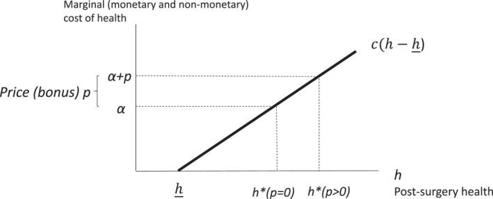 FIGURE 1
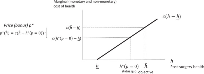 FIGURE 2
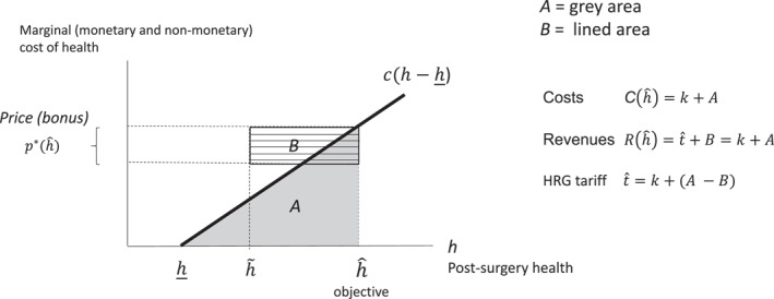 FIGURE 3
| Mean | sd | min | max |
| |
|---|---|---|---|---|---|
| Hip replacement | |||||
| Cost, MFF adjusted (£) | 5859.08 | 1372.57 | 1659.96 | 11,293.33 | 128 |
| Risk‐adjusted post‐operative health (OHS) | 39.42 | 1.13 | 34.41 | 42.07 | 128 |
| Pre‐operative health (OHS) | 17.06 | 1.66 | 12.05 | 21.29 | 128 |
| Risk‐adjusted health gain (OHS) | 21.44 | 1.13 | 16.43 | 24.08 | 128 |
| Risk‐adjusted post‐operative health (EQ‐5D) | 0.79 | 0.03 | 0.67 | 0.85 | 128 |
| Pre‐operative health (EQ‐5D) | 0.32 | 0.06 | 0.14 | 0.45 | 128 |
| Risk‐adjusted health gain (EQ‐5D) | 0.43 | 0.03 | 0.31 | 0.50 | 128 |
| Knee replacement | |||||
| MFF adjusted total cost (£) | 5798.55 | 1231.76 | 2386.37 | 9827.19 | 128 |
| Risk‐adjusted post‐operative health (OHS) | 35.58 | 1.04 | 31.54 | 38.21 | 128 |
| Pre‐operative health (OHS) | 18.41 | 1.49 | 13.64 | 22.27 | 128 |
| Risk‐adjusted health gain (OHS) | 16.38 | 1.04 | 12.33 | 19.00 | 128 |
| Risk‐adjusted post‐operative health (EQ‐5D) | 0.74 | 0.02 | 0.67 | 0.81 | 128 |
| Pre‐operative health (EQ‐5D) | 0.39 | 0.06 | 0.20 | 0.52 | 128 |
| Risk‐adjusted health gain (EQ‐5D) | 0.32 | 0.02 | 0.25 | 0.39 | 128 |
| I | II | III | IV | V | VI | VII | VIII | IX | |
|---|---|---|---|---|---|---|---|---|---|
| Observed costs and health | |||||||||
| Hospital cost (£) | 5859 | 5859 | 5859 | 5859 | 5859 | 5859 | 5859 | 5859 | 5859 |
| , OHS | 39.42 | 39.42 | 39.42 | 39.42 | 39.42 | 39.42 | 39.42 | 39.42 | 39.42 |
|
| |||||||||
| % Fixed costs | 80% | 80% | 80% | 80% | 80% |
|
| 80% | 80% |
| Fixed costs (£) | 4687 | 4687 | 4687 | 4687 | 4687 | 4101 | 5273 | 4687 | 4687 |
| Variable costs (£) | 1172 | 1172 | 1172 | 1172 | 1172 | 1758 | 586 | 1172 | 1172 |
| (OHS) | 34.00 | 34.00 | 34.00 | 34.00 | 34.00 | 34.00 | 34.00 |
|
|
| Cost function parameter c (£) | 79.8 | 79.8 | 79.8 | 79.8 | 79.8 | 119.7 | 39.9 | 200.4 | 400.2 |
| Objective of the funder , OHS | 40.55 | 40.55 | 40.55 |
|
| 40.55 | 40.55 | 40.55 | 40.55 |
| Price p per health improvement (£) | 90.1 | 90.1 | 90.1 | 135.2 | 180.3 | 135.2 | 45.1 | 226.4 | 452.2 |
| Additional costs | |||||||||
| (£) | 6399 | 6399 | 6399 | 6707 | 7040 | 6668 | 6129 | 6761 | 7209 |
| (£) | 540 | 540 | 540 | 848 | 1181 | 809 | 270 | 902 | 1350 |
| Revenues | |||||||||
| (OHS) | 38.29 |
|
| 38.29 | 38.29 | 38.29 | 38.29 | 38.29 | 38.29 |
| (£) | 3656 | 3656 | 3656 | 5560 | 7515 | 5483 | 1828 | 9181 | 18,337 |
| (£) | 204 | 407 | −204 | 382 | 611 | 306 | 102 | 512 | 1022 |
| HRG tariff (£) | 6195 | 5991 | 6602 | 6325 | 6429 | 6363 | 6027 | 6250 | 6187 |
| I | II | III | IV | V | VI | VII | |
|---|---|---|---|---|---|---|---|
| Observed costs and health | |||||||
| Cost (£) | 5859 | 5859 | 5859 | 5859 | 5859 | 5859 | 5859 |
| , EQ‐5D (out of 100) | 79.09 | 79.09 | 79.09 | 79.09 | 79.09 | 79.09 | 79.09 |
| Assumptions | |||||||
| % Fixed costs | 80% | 80% | 80% |
| 70% | 70% | 70% |
| Fixed costs | 4687 | 4687 | 4687 | 4101 | 4101 | 4101 | 4101 |
| Variable costs | 1172 | 1172 | 1172 | 1758 | 1758 | 1758 | 1758 |
| 66.65 |
|
| 72.45 | 72.45 | 72.45 | 72.45 | |
| Cost function parameter c (£) | 15.1 | 25.8 | 53.2 | 79.7 | 79.7 | 79.7 | 79.7 |
| Objective of the funder | 81.99 | 81.99 | 81.99 | 81.99 |
| 84.89 |
|
| Price p per health improvement (£) | 43.9 | 74.7 | 154.2 | 231.2 | 462.5 | 462.5 | 1016.2 |
| Additional costs | |||||||
| (£) | 6469 | 6680 | 7106 | 7730 | 10,271 | 10,271 | 19,082 |
| (£) | 610 | 821 | 1247 | 1871 | 4412 | 4412 | 13,223 |
| Revenues | |||||||
| 76.19 | 76.19 | 76.19 | 76.19 | 76.19 | 76.19 | 76.19 | |
| (£) | 3601 | 6123 | 12,639 | 18,958 | 39,258 | 39,258 | 93,323 |
| (£) | 255 | 433 | 894 | 1341 | 4023 | 4023 | 15,898 |
| HRG tariff (£) | 6214 | 6247 | 6212 | 6389 | 6247 | 6247 | 3184 |
| Cost effectiveness | |||||||
| QALY improvement for 0.01 EQ‐5D | 0.1149 | 0.1149 | 0.1149 | 0.1149 | 0.1149 |
|
|
| QALY improvement | 0.3332 | 0.3332 | 0.3332 | 0.3332 | 0.6664 | 0.5974 | 1.3133 |
| Cost per QALY | 1831 | 2463 | 3743 | 5614 | 6620 | 7385 | 10,069 |
- —National Institute for Health and Care Research10.13039/501100000272
Peer Reviews
No public reviews on file for this paper yet. If you reviewed it on a platform where reviews are public (OpenReview, ICLR, NeurIPS, ICML), you can paste yours below so the community can read it here.
Videos
No videos yet. Explain this paper in a talk, walkthrough, or lecture? Add one.
Taxonomy
TopicsHealth Systems, Economic Evaluations, Quality of Life · Healthcare Policy and Management · Primary Care and Health Outcomes
Introduction
1
Reimbursement to healthcare providers are often based on the number of patients with a particular diagnosis or treatment. Activity‐based financing based on Diagnosis Related Groups (DRGs) remains dominant across OECD countries. There are however a number of concerns with these payment mechanisms including under‐treatment, if providers skimp on quality, or over‐treatment if rewarding activity induces providers to engage in costly activity that does not improve health. The fundamental issue is that payment based on activity alone does not take into account the value of treatments being provided. One intuitive response is to make prices reflect the additional value of the health outcomes produced. This would require measuring the outcome of treatment in terms of health gain and paying a bonus that rewards health improvements. Payment based on health outcomes has long been discussed and sometimes advocated as a natural development of activity‐based financing (Dunbar‐Rees 2018).
The appeal of outcome‐based payment systems is that they reward what ultimately matters, health gains. However, health outcomes are difficult to measure. Some commonly available indicators, such as mortality and readmission, only apply to treatments where there is a sufficient incidence of failure and high volume. Moreover, both mortality and readmission rates measure health on one tail of the outcome distribution. More recently, broader measures of health gains have been collected in the form of patient‐reported outcome measures (PROMs) for common procedures such as hip and knee replacement (NHS England 2013; Gutacker et al. 2013). These measures consider health gains across the whole distribution.
Even with accurate health measures, there is lack of consensus on how the incentive bonus should be set. The evidence suggests that providers, hospitals in particular, tend to have limited response to pay‐for‐performance schemes (Cashin et al. 2014; Milstein and Schreyoegg 2016; Mendelson et al. 2017).1 A possible explanation is that the size of the bonus was relatively small (about 5% of hospital revenues with some variation across schemes and countries (Cashin et al. 2014)), and so insufficient to induce changes in provider behavior.2
This study adopts a contract theory approach to examine the appropriate size of the bonus to inform practical implementation of pay‐for‐performance (P4P) schemes that reward health outcomes. First, we provide a simple but general model for the design of an incentive scheme that rewards health gains, based on key parameters related to patient health benefits and provider costs (Section 2). Second, the model is calibrated with health outcome and cost data from two elective procedures, hip and knee replacement, to illustrate the applicability of the framework and show the sensitivity of the bonus to different assumptions on benefits and costs (Section 3). The study bridges the gap between economic theory and policy, and informs the design of P4P schemes where health is observable and measured accurately. The model takes a representative provider approach. We show that the findings are robust to extending the analysis to heterogeneous providers (Section 4).
In line with the literature (Ellis and McGuire 1986; Chalkley and Malcomson 1998), we assume that providers are altruistically or intrinsically motivated and choose a level of quality that trades off the benefits from higher quality against its costs. We then model the purchaser decision regarding the bonus. We first adopt a positive economics perspective where the purchaser specifies a bonus to achieve a health objective or target based on the observed empirical distribution across providers (e.g., increasing the average health gain by one standard deviation or to the level of health in the top quartile or quintile of the health distribution).
We then adopt a cost‐effectiveness analysis approach and provide a framework to explore whether the introduction of the bonus is cost‐effective. We compare the value of the health benefits generated by the scheme against the additional provider costs, which in our model coincide with the additional reimbursement made by the funder of health services (i.e., the National Health Service). Finally, we use a welfare function approach and derive the optimal pricing rule that induces a level of health which maximizes the difference between the value of patient benefits and provider costs. We also relate this approach to cost‐effectiveness analysis.
Throughout the analysis, we assume that the bonus is in addition to the basic activity‐based price (Healthcare Resource Groups (HRG) tariff, the English equivalent to DRG tariff), which can be adjusted to ensure that provider revenues cover treatment costs. This implies that the amount reimbursed by the purchaser to the provider is always equal to the provider's costs. This approach is broadly in line with several health systems that use DRGs as basis for reimbursement. The DRG tariff is generally based on past national average hospital costs for a specific diagnosis/treatment (with a one‐ or 2‐year lag): a form of yardstick competition (Shleifer 1985). In England, the introduction of P4P schemes for hospitals (known as Best Practice Tariffs) have combined the introduction of the bonus with a reduction of the basic HRG tariff. This was the case for Best Practice Tariffs that incentivized quality for stroke (Kristensen et al. 2016) and hip fracture (Grašič et al. 2025).
Given our applied focus, we express the bonus as a function of the post‐operative health before the introduction of the bonus, and the target post‐operative health after the introduction of the bonus, as this information is available or chosen by the purchaser. In our positive analysis, we show that the optimal pricing rule for the purchaser is to choose a bonus that reflects the difference between the marginal cost of post‐operative health before the policy intervention and the marginal cost of post‐operative health at the target level of health set by the purchaser (i.e.., post policy).
We show that that the incentive scheme is cost‐effective if the cost‐effectiveness ratio is below a given threshold, where additional health benefits are compared to additional provider costs, which in our model coincide with the additional reimbursement to the provider. Under a welfare‐function approach, we also show that the optimal price per unit of health is equal to the marginal benefit from health, weighted by the opportunity cost of public funds, net of provider marginal cost of health before the introduction of the bonus payment.
Using data from hip and knee replacement in England we calibrate the model for the average provider with respect to two key parameters, provider costs and post‐operative health. We compute the bonus payments that the purchaser would have to make to achieve target levels of post‐operative health equivalent to improvements of one or two standard deviations of the health distribution observed across providers. To infer the shape of the cost function for the average provider, we make assumptions related to fixed and variable costs. In our calibration for hip replacement, we find that the price for one unit of health improvement as measured by the Oxford Hip Score (OHS) to achieve an improvement of 1.13 points on the OHS scale (equivalent to one standard deviation observed in the empirical distribution) ranges between £45 and £226 under different assumptions related to the cost function. For knee replacement, the price for one unit of health improvement as measured by the Oxford Knee Score (OKS) to achieve an improvement of 1.06 points on the OKS scale (equivalent to one standard deviation observed in the empirical distribution) ranges between £72 and £254 under different assumptions related to the cost function. The price doubles for a health target of two, rather than one, standard deviation improvement.
When we evaluate the health benefit in quality‐adjusted life years (QALYs), for which there are official estimates of the purchaser willingness‐to‐pay in the English NHS, we generally find that the introduction of the bonus is cost effective, even at high levels of health targets. In turn, this implies that under a welfare function approach, the optimal health target is high and so is the price per unit of health improvement.
Our analysis makes explicit which cost and benefit parameters are required for practical implementation of paying for health schemes. Even for a positive analysis where the purchaser sets an ad hoc health target, the approach requires assumptions about the marginal cost of health improvement both at the status quo and at the target level of health. One approach is to take an accounting perspective and gather data and estimate the cost of plausible hospital interventions to increase post‐operative health (e.g., through an estimate of the time that health workers would have to devote to implement such interventions). Another approach is to conduct empirical analyses to estimate the marginal cost of increasing health for specific procedures.
Related Literature
1.1
There is a relatively small literature which calibrates theoretical models of incentive schemes for healthcare providers. The closest study is Kristensen et al. (2016) that presents a stylized model for hospital price setting for (three) process measures of quality. The model is calibrated using features of the Best Practice Tariffs scheme for emergency stroke care in the English NHS that rewarded hospitals for ensuring treatment in an acute stroke unit, rapid brain imaging, and provision of thrombolytic medication to some patients. Our study differs in several ways. First, we investigate pricing schemes that stimulate quality by targeting health outcomes, rather than process measures of quality. Second, we derive the pricing rule as a function of pre‐policy intervention parameters. Third, we include a positive analysis and a cost‐effectiveness approach, in addition to a welfare analysis. Finally, our calibration applies to elective rather than emergency care.
Lisi et al. (2020) provide a theoretical analysis of P4P to encourage reductions in mortality and readmission rates when patients differ in severity, hospitals compete on quality, and risk‐adjustment is incomplete. They show that P4P can weaken or strengthen hospitals' incentive to provide quality. Since patients with higher severity are more likely to exercise choice, this introduces a patient composition effect which alters quality incentives and is stronger in more competitive environments. They calibrate the model based on the Premier Hospital Quality Incentive Demonstration introduced by the Centers for Medicare & Medicaid Services in 2012 and the Hospital Readmission Reduction Program. Unlike our paper, no optimal pricing rule is derived. Sa et al. (2019) model hospital competition in the presence of excess demand and waiting times. They calibrate the model using waiting times and volume for cataract surgery in the English NHS to compare different solution concepts, but again no optimal pricing is derived.
Chalkley and Malcomson (2003) investigate the scope for refining DRG hospital payments by allowing for cost sharing. They show that if providers differ in costs and there is asymmetric information, then total payment can be reduced by cost sharing. Calibration with Medicare data suggests that cost sharing can generate cost savings that range from 7% for treatments with low‐cost variation to 60% for those with high‐cost variation. By contrast, we assume that costs cannot be contracted on.
There is a larger theoretical literature investigating provider incentives in relation to quality and cost containment, which derives qualitative insights on provider behavior and the features of optimal payment systems under a range of assumptions (see seminal studies by Ellis and McGuire 1986; Chalkley and Malcomson 1998; Siciliani 2018, for a review). A smaller literature focuses specifically on P4P, in relation to multitasking (tunnel vision) and gaming or misreporting (see Eijkenaar 2013, for an overview of key design issues). Eggleston (2005) shows that targeting some quality dimensions comes at the cost of reducing untargeted quality dimensions when qualities are substitutes, though cost sharing can mitigate this. Kaarboe and Siciliani (2011) show that this implies that the price is reduced as a result. Sherry (2016) finds that when P4P programmes reward multiple healthcare services in a setting characterized by joint production, the impact on both rewarded and unrewarded services is ambiguous. Kuhn and Siciliani (2009), (2013) show that gaming also generally leads to lower‐powered incentive schemes. Mak (2018) studies a managed healthcare market with two differentiated hospitals. It analyses the interaction of P4P schemes on contractible quality with other features of the market, such as copayment and consumers' misperception of quality. These studies do not provide calibrations, which is a key focus of our paper.
Model
2
We adopt a contract theory approach (Ellis and McGuire 1986; Chalkley and Malcomson 1998) in which the principal (purchaser) can choose a payment mechanism that influences the choice of the agent (provider). Our focus is how the payment of a health‐related bonus affects the provider's decision concerning patient health gain from subsequent treatment.
In Section 2.1, we analyze the provider's choice of patient post‐operative health conditional on the payment rule. The provider therefore takes the reimbursement rule set by the purchaser as given. This consists of the basic DRG tariff and the bonus payment. We use a stylized setting of a representative provider that can expend costly effort to achieve better health outcomes. We implicitly assume that all patients are the same or, equivalently, that health measures are risk‐adjusted. This is important as the lack of risk adjustment could expose the provider to losses (or profits) that are due to external factors.
In Section 2.2, we consider the purchaser perspective under three different approaches. In designing the contract, the purchaser always anticipates the effect of the bonus payment on provider behavior. First, we consider how a purchaser can design a bonus to achieve a target level of health, which we label positive analysis (Section 2.2.1). Second, we investigate whether the introduction of a bonus is cost‐effective (Section 2.2.2). Third, we design a bonus which maximizes welfare (Section 2.2.3) defined as patient health benefits minus provider costs.
Formally, at time t = 1, the purchaser chooses the payment mechanism. At time t = 2, the hospital chooses the level of health provided to the patients. We solve by backward induction.Definition of variables h Patient post‐operative health h0 Patient pre‐operative health h˜ Threshold health level above which payment is received h_ Level of health over which improving health is costly to the provider hˆ Purchaser health target objective H(h) Patient life‐time health gain t Prospective DRG/HRG fixed price p Bonus payment per unit of health improvement C(h) Provider cost function k Fixed treatment cost component c Parameter related to marginal cost of health improvement α Degree of provider motivation (altruism) W Willingness to pay for health improvement δ Opportunity cost of public funds λ Cost‐effectiveness threshold
The Provider Perspective
2.1
We define h as patient post‐operative health as determined by provider's effort to improve health and measured (at some point, e.g. six months) after the surgery.3 Pre‐operative health is h0.
Revenues
2.1.1
The provider is paid through a prospective Diagnosis Related Group (DRG) or Healthcare Resource Groups (HRG) tariff t and a health‐outcome related bonus p that is linear in health improvement.4 Hospital revenue R(h) is:
where h˜ is a threshold health level decided by the purchaser and h is patient post‐operative health.
As an example, consider a patient in need of a hip replacement and that post‐operative health is measured with the Oxford Hip Score (OHS) on a 0–48 scale with higher values indicating better health. Suppose that the health threshold h˜ has an OHS of 30, that post‐operative health has a score of h=38, and that the price for one point of health improvement on the OHS scale is £100. Then hospital bonus payment from treating a patient, in addition to the HRG tariff, is ph−h˜=100(38−30)=£800. Equation (1) also encompasses the scenario where the provider has a penalty, rather than a bonus. This can be achieved by setting a threshold h˜ which is sufficiently high.5
The provider takes the HRG tariff t and the bonus p as given. This is plausible because the reimbursement rules are set by the purchaser at the beginning of the financial year. In Section 2.2, we discuss how the purchaser sets both the value of the tariff and the bonus payment.
Costs
2.1.2
We assume that the provider has the following cost function for treating a patient:
where k is a fixed treatment cost component, which is independent of health gain (e.g., the cost of an operating theater, the time of surgeons and nurses, anesthetist) and K(h) is the additional cost of improving the health of the patient, which includes both monetary costs (due to more expensive technology, medicines) and non‐monetary costs (e.g., time of nurses and doctors).6 We assume that the cost is increasing and convex in health. Higher levels of health increase costs, ∂K(h)/∂h>0, at an increasing rate, ∂2K(h)/∂h2>0. While some health improvements are relatively easy to generate at low additional cost or even costless, it is increasingly costly for the provider to achieve additional health gains, which is captured by convexity of the cost function. For example, going beyond standard care would require additional rehabilitation, physiotherapy, follow‐up with the patient to ensure adherence with protocols and guidelines, etc.
To obtain a closed‐form solution, which we use for the calibration, we assume that the cost function is quadratic in h:
where c>0 is a parameter related to the marginal cost of a health improvement, and h_ is the level of health over which improving health is costly for the provider. We could set the latter at the pre‐operative health, h_=h0. However, it is likely that providers with low level of costly efforts might still be able to achieve post‐operative health that is higher than the pre‐operative health. We therefore allow for the possibility that improving health up to h_ does not generate any additional costs on top of the fixed treatment costs k.7
Motivation
2.1.3
We assume that the provider is motivated (due to altruism, intrinsic motivation toward quality or other reasons) and will improve the health of the patient even if not financially rewarded (as in Ellis and McGuire 1986; Chalkley and Malcomson 1998). We capture this motivation as B(h), which is increasing in health. We assume the following linear functional form:
where α is the degree of motivation. This parameter could also be interpreted more broadly as any source of motivation. In addition to altruism and intrinsic motivation, it encompasses other incentives to improve health that arise from monitoring and auditing mechanisms. For example, regulators can analyze quality indicators and conduct audits on a regular basis to ensure minimum standards. This parameter plays a critical role in the analysis, because higher levels of motivation imply higher levels of health, which reduces the scope to introduce financial incentives (as highlighted more comprehensively in Section 2.2). As illustrated below, if other regulatory mechanisms increase quality before the P4P bonus is introduced, the scope of P4P is reduced.
Hospital Payoff Function
2.1.4
We assume that the payoff function of the provider V(h,p) from treating the representative patient includes both financial and non‐financial motives, and is additively separable in the motivation component B(h) and financial surplus π(h,p)=R(h,p)−C(h):
Maximizing with respect to the patient post‐operative health h, the provider chooses the level of health h∗ which satisfies the first‐order condition:
The provider balances the marginal monetary and non‐monetary benefits of increasing the patient's health against the marginal costs of health improvement. The second‐order condition is ∂2V(h;p)/∂h2=−c<0. Changes in the basic DRG tariff t do not affect the level of health. This is because the tariff t is a lump‐sum payment that does not depend on the care provided. It is only the bonus payment per unit of health p that affects the patient's level of health. Higher levels of motivation α increase post‐operative health, while a higher marginal cost c reduces health.
The hospital's choice of patient post‐operative health is:
which is increasing in the bonus payment p.8 Figure 1 illustrates the solution, and shows that post‐operative health is higher in the presence of a bonus, h∗(p>0), than in the absence of a bonus, h∗(p=0)=h_+α/c.9
Provider choice of post‐surgery health.
The Purchaser Perspective
2.2
We discuss three different approaches the purchaser might adopt in setting up the bonus scheme.
Positive Analysis
2.2.1
First, suppose that the purchaser would like to achieve a health objective, given by hˆ. A higher bonus p induces a higher level of post‐operative health, while a higher DRG tariff t does not affect health. Because we assume that the number of patients is unaffected by h, the DRG tariff acts as a lump‐sum payment, which is independent of the care provided. The price that implements the objective set by the purchaser is found by equating provider's choice of post‐operative health with purchaser's health objective, h∗(p)=hˆ:
Thus, the bonus should be set equal to the marginal cost of post‐operative health at the required target level of health, net of the degree of provider motivation (in line with previous literature, Ellis and McGuire 1986; Chalkley and Malcomson 1998; Kristensen et al. 2016). The greater the degree of motivation, the smaller is the price required to induce the provider to achieve the target health objective.
We can also re‐write the incentive p as a function of post‐operative health in the absence of a bonus system (e.g., before the scheme is implemented or the status quo). In the absence of the scheme, post‐operative health is h∗(p=0)=h_+α/c, and hence
This is our main result, which will be used in the calibration of the payment system in Section 3. It suggests that the price should be set equal to the difference in the provider marginal cost evaluated at the target level of post‐operative health that the purchaser would like to achieve, chˆ−h_, and the marginal cost evaluated at the level of health before the scheme is introduced, ch∗(p=0)−h_. Figure 2 illustrates the solution. We plot post‐operative health on the x‐axis, and the marginal cost of post‐operative health on the y‐axis. We then evaluate the marginal cost of post‐operative health before the policy intervention (status quo) and after the policy intervention (at the health target). The price (bonus) per unit of post‐operative health is the difference in these two marginal costs.
Price designed by the funder to achieve a given health objective.
Provider cost at the new equilibrium following the introduction of the bonus is:
Provider costs are higher at the health target hˆ, and the purchaser has to take these additional costs into account. We have assumed that the purchaser has to ensure that provider costs are covered by provider revenues. Part of the costs are already covered through the bonus payment. The purchaser can then set the HRG tariff equal to the difference between provider costs and provider revenues from the bonus:
Figure 3 illustrates the solution, showing revenues, costs and the HRG tariff for a given health objective hˆ that ensures zero profits. Provider variable costs are given by the gray area A. Total costs are given by the fixed cost k plus the variable costs A. The revenues from the bonus are given by area B. Given that total revenues have to be equal to provider costs, the HRG tariff is given by k+(A−B), the fixed cost minus the difference between the variable costs and the revenues from the bonus. In summary, provider revenues from the bonus and the HRG tariff cover hospital costs when the provider chooses a post‐operative health that is equal to the purchaser health target.
Revenues, costs and basic (HRG) tariff.
Cost‐Effectiveness Analysis
2.2.2
In this section, we provide a framework to assess when the introduction of a P4P scheme that rewards health is cost effective. This approach is relevant in budget‐constrained health systems to evaluate whether the extra health gain is worth the cost of achieving it. As shown in the previous section, provider costs increase as a result of the new health target hˆ. The difference in provider costs before and after the introduction of the bonus is given by:
Since the purchaser sets the payment such that provider revenues are equal to provider costs, the change in purchaser payment is identical to the change in provider costs.
We define H(h) as patient life‐time gain in health, for example measured in QALYs, arising from a post‐operative health equal to h. The difference in health benefit with and without the bonus is:
The cost‐effectiveness ratio is:
New treatments or interventions are assessed against a threshold value λ for the cost‐effectiveness ratio. The introduction of the bonus payment is cost‐effective if the cost‐effectiveness ratio is below the threshold, ΔC/ΔH<λ and is not cost‐effective if above the threshold, ΔC/ΔH≥λ.
Normative Analysis
2.2.3
In this section, we adopt a conventional welfare economics perspective where a purchaser makes choices that maximize patient benefits, net of provider costs, where the latter are weighted by the opportunity costs of public funds. We also relate this approach to the cost‐effectiveness analysis outlined in the previous section. Define Ω(h) as welfare, δ as the opportunity cost of public funds (or the opportunity cost of the overall health budget) and W as the willingness to pay for health improvement. Welfare is then given by:
The optimal level of post‐operative health satisfies the first‐order condition ∂Ω(h)/∂h=0, or more extensively:
so that, at the optimal level of post‐operative health, the marginal benefit from health gain is equal to the marginal cost. The closed‐form solution for the welfare‐maximizing level of health is
Comparing the welfare‐maximizing level of health, hw, with that chosen by the provider, h∗(p), we can compute the bonus price that implements the welfare‐maximizing level of health10 ^:^
The optimal price is equal to the marginal benefit from a health gain, weighted by the opportunity cost of public funds, net of provider marginal cost of health before the introduction of the bonus.
We can also relate this analysis with the cost‐effectiveness approach presented in the previous sub‐section. For simplicity, set λ=W/1+δ, and re‐define welfare as λ×H(h)−C(h), which within the cost‐effectiveness literature is known as the net monetary benefit (Stinnett and Mullahy 1998; Hoch et al. 2002). We can re‐write the optimal post‐operative health as hw=h_+λc∂Hhw∂h. Starting from a level of post‐operative health below hw, then any improvement in health is cost‐effective as λ×∂H(h)∂h−∂C(h)∂h>0 or, equivalently,
and any improvement above hw is not cost‐effective as ∂C(h)/∂h∂H(h)/∂h≥λ.
Calibration
3
To illustrate how the bonus scheme might work in practice, we calibrate the model using English hospital data for two common elective procedures. We use cost and health data for patients receiving a primary unilateral elective hip or knee replacement in 2016–2017. To measure hospital costs, we employ reference costs reported annually by hospitals at the Healthcare Resource Group level, the English equivalent to DRGs.11
For each hospital we also measure risk‐adjusted patient health status 6 months after the surgery.12 We use the Patient Reported Outcomes Measure dataset constructed from patient survey responses.13 We have two measures of patient‐reported health status for each procedure. The first is a condition‐specific measure known as the Oxford Hip Score (OHS) for hip replacement and Oxford Knee Score (OKS) for knee replacement. These measures different dimensions of pain and mobility, and is based on 12 questions giving a score ranging from 0 to 48, with higher values indicating better states of health. The second health measure is the generic EQ‐5D instrument, which asks patient to report whether they have no, some or extreme problems on five health dimensions: mobility, pain & discomfort, anxiety & depression, ability to wash and dress themselves, and ability to carry out their usual activities. The answers form a health profile for which utility values have been elicited from the UK general population. EQ‐5D utility values range from −0.594 to 1. They can be used to calculate quality‐adjusted life years (QALYs). Descriptive statistics are reported in Table 1.
Hip Replacement
3.1
The average cost for a hip replacement across 128 public hospitals (Trusts) in England in 2016–2017 was £5859. The average risk‐adjusted post‐operative health was 39.42 as measured by the Oxford Hip Score. 14
We have to make several assumptions to recover the marginal cost parameter c, which can be interpreted as the difference in the marginal cost for one unit of health improvement.15 Although we cannot observe the marginal cost, we can gather information on some fixed cost components from the literature.16 In the baseline calibration (column I of Table 2), we assume that 80% of the costs are fixed, which implies that variable costs account for £1172. There remains uncertainty around the variable costs. Table 1 suggests that the standard deviation of the total provider costs is £1372 (23.4% of the mean). We explore the sensitivity of the results to both lower and higher percentages (70% and 90%). We also need to make assumptions about the value of post‐operative health above which it is costly to increase health, defined with h_ in Section 2, which is another source of uncertainty related to marginal costs. We assume that h_ is equal to 34 OHS, which is just below the minimum post‐operative health observed in the hospital sample (34.41 OHS). We explore below the sensitivity of the results to lower or higher values. Given that ch∗(p=0)=c2h∗(p=0)−h_2, we can re‐cover the cost parameter c=2ch∗(p=0)h∗(p=0)−h_2=21172(39.42−34)2=£79.8.
In our baseline, we assume that the purchaser sets the objective of the scheme at a post‐operative health, hˆ, equal to 40.55 OHS. This corresponds to an improvement of 1.13 OHS which is one standard deviation in post‐operative health across 128 providers in 2016–2017 (with a maximum of 42.07 OHS). Using (23), the price per unit of health improvement (one OHS) to achieve the objective hˆ=40.55 OHS is equal to p∗hˆ=chˆ−h∗(p=0)=£90.1. The cost of a hip replacement at the higher post‐operative health is Chˆ=£6399, and the additional cost relative to pre‐policy intervention is ΔC=Chˆ−Ch∗(p=0)=£540.
In terms of provider revenues, the purchaser must decide the level of post‐operative health h˜ (see (1)) over which the purchaser pays for additional health improvements. We set this level at h˜=38.29, which is equal to the pre‐policy post‐operative health minus one standard deviation in post‐operative health (39.42−1.13). This threshold is somewhat arbitrary. We have assumed that any additional provider revenues arising from the bonus trigger a reduction in the HRG tariff. In this specific case, the additional revenues from the bonus are p∗hˆ×hˆ−h˜=90.1×(40.55−38.29)=£204. Given that the total cost of a hip replacement is £6399, the basic HRG tariff to ensure that the provider breaks even is equal to thˆ=£6195.
The purchaser could instead choose the lower post‐operative health threshold h˜=36.06 (three standard deviations in post‐operative health). Column II of Table 2 suggests that the optimal price remains unchanged given that the health objective is the same. However, the provider receives larger revenues from the bonus, equal to p∗hˆ×hˆ−h˜=90.1×(40.55−36.06)=£407, and these are accompanied by a lower basic HRG tariff equal to £5991, which ensures again that total revenues are equal to provider costs (£6399).17
A More Ambitious Target
3.1.1
In columns IV and V of Table 2, we assume that the purchaser sets a more ambitious target with a post‐operative health which is respectively 1.5 and 2 standard deviations higher (rather than one). If the other assumptions remain the same, this implies a price for unit of OHS improvement now equal to £135.2 and £180.3, respectively.
In the first (second) scenario, costs increase to £6707(£7040), which implies an additional cost of £848 (£1181), relative to the introduction of the scheme. Under the same assumptions as in column I in Table 2, the revenues from the bonus are now £382 (£611), which implies that the purchaser reduces the basic HRG tariff to £6325 (£6429) to ensure that the costs are covered.
As intuitively expected, the price per unit of health improvement increases with the ambition of the target. The higher level of health increases costs and revenues, and the purchaser therefore needs to adjust the basic HRG tariff to reflect the higher level of the cost.
Different Cost Function
3.1.2
We have assumed that 80% of costs are fixed. In columns VI and VII we make the same assumptions as in column I but change the proportion of costs that are fixed to 70% and 90%, respectively. The price per unit of health improvement now increases (reduces) to £135.2(£45.1). The cost parameter c also increases (reduces) to £119.7 (£39.9). Driven by the higher tariff, the additional revenues from the bonus also increase (reduce). The basic HRG tariff also increases (reduces), despite the higher bonus, and this is driven by the higher (lower) additional costs ΔC=£809(£270).
We can also vary the minimum level of post‐operative health over which costs increase, which we have set at h_=34 OHS. In columns VIII and IX, we maintain the same assumptions as in column I but increase h_ to 36 and 37, respectively. This implies an increase in the cost function parameter c to £200.4 and £400.2, which translate into a higher price per unit of health improvement equal to £226.4 and £452.2. The higher marginal cost of a health improvement implies that costs at the new health target are £6761 and £7209, respectively. The revenues from the bonus are now £512 and £1022, with the basic HRG tariff being re‐adjusted to cover the costs.
Cost‐Effectiveness Analysis
3.1.3
To investigate whether the introduction of the incentive scheme is cost‐effective, we set the health objective of the purchaser as a function of EQ‐5D utility scores. Following similar steps as above, column I of Table 3 provides our baseline. The pre‐policy post‐operative health now gives a EQ‐5D utility score of 0.79 and the purchaser objective is 0.82.18 To simplify the presentation, we measure post‐operative health with the EQ‐5D utility score multiplied by 100, so that a post‐operative health of 0.79 is measured as h=79.
Under the assumption that 80% of the costs are fixed, and h_=66.65 (i.e., 0.6665 EQ‐5D utility score, about the minimum level observed in the hospital sample), then the optimal price is £43.9 per unit of health improvement (0.01 EQ‐5D utility score). With a payment health threshold of 76 (0.76 EQ‐5D utility score), the hospital revenues from the bonus are £255, and the basic HRG tariff is £6214, with an overall provider cost of £6469.
We assume that the health gain over the patient life span for a 0.01 EQ‐5D utility score improvement is 0.1149 QALYs (ranging from 0.103 under more conservative estimates to 0.126), computed as follows. We follow Briggs et al. (2004) and Jenkins et al. (2013) and draw from the expected remaining years of life of the general population from Office for National Statistics Life Tables, and use the expected life of patients with the average age of our empirical sample in 2016/17, amounting to 18 years. We then adjust for the mortality risk in each of these years.19 Finally, we discount future health gains using a time preference discount rate ranging from 1.5% (Claxton et al. 2011) to 3.5% as recommended by HM Treasury. Under these different assumptions the QALY improvement from hip replacement ranges from 0.103 to 0.126 QALYs (see also Appleby et al. 2013; Schmitz et al. 2019).
In terms of cost effectiveness, the incremental cost per QALY is £1831, suggesting that the introduction of the scheme is cost effective, well below the conventional thresholds used in economic evaluation of healthcare programmes (Claxton et al. 2015; Lomas et al. 2019).
In column II‐VI we investigate whether this result is robust to less favorable assumptions of the cost function. In columns II and III of Table 3, we increase h_ to higher values, which increase the cost parameter c from £15.1 to £25.8 and £53.2, leading to the higher prices of £74.7 and £154.2. In column IV we further increase the proportion of variable costs to 30%, which implies a price of £231.2. In column V we maintain the assumptions in column IV but set the health target at 84.89, equivalent to two standard deviation improvement. The price is 462.5 per unit of health improvement, revenues from the bonus are £4023, and an overall provider cost of £10271. Despite the very high costs (relative to pre‐policy level of £5859), the introduction of the bonus remains cost‐effective with a cost per QALY of £6620. Column VI uses the more conservative estimate of a QALY gain of 0.103 for a 0.01 EQ‐5D utility score improvement. The cost per QALY is £7385.
This analysis suggests that for the purchaser it is generally cost effective to set an ambitious health target.
Normative Analysis
3.1.4
Based on Section 2.2.3, we can compute the optimal level of post‐operative health which equates purchaser's marginal benefit with its marginal cost, given by hw=h_+1cW(1+δ)∂Hhw∂h. We choose the most conservative parameters with highest costs and lowest benefits in column VI of Table 3: 30% variable costs and h_=72.45, leading to c=£79.7; a QALY improvement from an increase in one unit of post‐operative health equal to 0.1030, so that ∂Hhw∂h=0.1030; and a willingness to pay for a QALY equal to W(1+δ)=£15000.
By substitution, we obtain an optimal level of post‐operative health equal to hw=91.8. This is equivalent to an improvement of more than four standard deviations in post‐operative health relative to the pre‐policy level, well above the maximum post‐operative health observed across providers equal to 85 (0.85 EQ‐5D).
Recall that the optimal pricing rule is p∗hw=W(1+δ)∂Hhw∂h−ch∗(p=0)−h_. The optimal price which implements the level of post‐operative health hw=91.8 is then equal to p∗hw=15000∗(0.1030)−(79.7)79.09−72.45=£1016. The results are in column VII of Table 3. The cost of a hip replacement at such high levels of post‐operative health is about three times the cost at the baseline, £19082. Most of hospital revenues arise from the bonus, £15898, and the remaining from the HRG tariff, £3184. The incremental cost per QALY relative to the baseline (given by ΔCΔH=Chˆ−Ch∗(p=0)Hhˆ−Hh∗(p=0)) is further increased, and equal to £10069. The marginal cost‐effectiveness ratio evaluated at the optimal post‐operative health is instead ∂Chw/∂h∂Hhw/∂h=chw−h_0.1030=79.791.8−72.450.1030≈15000=W(1+δ), which is higher than the incremental cost‐effectivness ratio. The result that the marginal cost‐effectiveness ratio is equal to the purchaser willingness to pay holds by construction because the optimal price is computed such that the marginal benefit equates its cost.
We have chosen conservative measures of parameter values. Both higher benefits or lower costs would increase further the optimal post‐operative health set by the purchaser.
Knee Replacement
3.2
We replicate the analysis for knee replacement. The findings are qualitatively and quantitatively similar to those obtained for hip replacement. The price for one unit of health improvement as measured by the Oxford Knee Score (OKS) to achieve an improvement of 1.06 points on the OKS scale (one standard deviation) ranges between £72 and £254 under different assumptions on costs. See Appendix for details.
Heterogeneity Across Providers
4
In this section, we extend the analysis to a set‐up where hospitals differ in the marginal cost of improving health. We assume that the purchaser uses the same health‐related bonus p and DRG tariff t, as described in (1), for all providers. We assume that the cost function is:
where e is a parameter denoting provider type and is distributed with cumulative function F(e) and density function f(e) over the support emin,emax with an expected value normalized to one, E(e)=∫eminemaxef(e)de=1. For a given bonus payment, the optimal level of post‐operative health by each provider is h∗(p,e)=h_+(p+α)ec. We assume that emax is the most efficient provider (lowest marginal cost) and emin is the least efficient provider (has highest marginal cost), with emax>1 and 0<emin<1.
Positive Analysis
4.1
Suppose that the purchaser would like to achieve an average health across providers equal to hˆ=Eh∗(p,e). The bonus payment that implements this target health is such that
which is given by:
where recall that E(e)=1 by assumption. The optimal bonus per unit of health improvement is the same as in (8). Given that, in the absence of a bonus, the expected health is equal to Eh∗(p=0,e)=∫eminemaxh_+αecf(e)de=h_+αc, we can re‐write this bonus payment as a function of post‐operative health in the absence of a bonus (e.g., before the scheme is implemented):
This result is qualitatively similar to Section 2 with a representative provider.
We assume that the DRG tariff tˆ is set such that the expected revenues across providers are equal to the expected costs. This is in line with DRG‐type reimbursement systems that set the DRG tariff equal to the average cost across providers. In turn, this implies that some providers will make a profit while others will make a loss.
The cost for provider e when the bonus payment is set at pˆ, after substituting h∗pˆ,e=h_+hˆ−h_e, is equal to
and the expected cost is equal to
Similarly, the revenues for provider e for a given DRG tariff t is equal to: Rpˆ,e=t+pˆh∗pˆ,e−h˜. More efficient providers have higher post‐operative health and revenues from the bonus payment. The expected revenue across providers is ERpˆ,e=t+pˆhˆ−h˜. The purchaser can then compute the DRG tariff that ensures that the expected revenues are equal to the expected costs across all providers:
More efficient providers have higher revenues but also higher costs. Whether more efficient providers have a higher financial surplus depends on:
which suggests that financial surplus increases with efficiency only if the degree of altruism is sufficiently low.
Cost‐Effectiveness Analysis
4.2
Given the target hˆ, the difference in provider expected costs before and after the introduction of the bonus is given by:
Similarly, the difference in expected health benefit with and without the bonus is:
where
The cost‐effectiveness ratio is then given by ΔE(C)/ΔE(H). Policy interventions are assessed against a threshold value for the cost‐effectiveness ratio. Letting λ denote this cost‐effectiveness threshold then the bonus is cost‐effective if ΔE(C)/ΔE(H)<λ and is not cost‐effective if instead ΔE(C)/ΔE(H)≥λ. The results are qualitatively similar to those derived in Section 2.2.2.
Normative Analysis
4.3
The welfare function is given by the difference between patient's benefits and the transfer to providers, weighted by the opportunity cost of public funds δ:
Welfare is maximized subject to the budget constraint that the expected revenues are equal to the expected costs across providers:
Substituting for the budget constraint, the optimal payment per unit of health improvement p is such that it satisfies the following first‐order condition:
Substituting ∂Ch∗(p,e),e∂h=α+p for any e, we can write the optimal payment per unit of health gain, denoted with pw as:
The optimal price is equal to the expected marginal benefit from a health gain, weighted by the opportunity cost of public funds, net of provider degree of motivation. The optimal pricing rule is analogous to the one obtained in Section 2.2.3, except that the marginal benefit is averaged across all providers. We can also re‐write the pricing rule as:
where the second term can be interpreted as the expected marginal cost across providers in the absence of a bonus, given that ∂Ch∗(p=0,e),e∂h=α. Again, the optimal pricing rule is qualitatively similar to Section 2.2.3 but with marginal benefit and cost averaged across providers.
The purchaser can then compute the optimal DRG tariff tw that ensures that the expected revenues are equal to the expected costs across all providers:
The DRG tariff ensures that on average providers do not make losses.
Calibration
4.4
Consider the baseline calibration for hip replacement (column I of Table 2). For the positive analysis, we assume that the purchaser's objective is to increase the average post‐operative health from 39.42 to 40.55 on the Oxford Hip Score scale (or one standard deviation in post‐operative health across hospitals). Given that the expected cost is ECh∗(p=0,e),e=k+c2α2, and that Eh∗(p=0,e)=h_+αc, we can re‐write the expected cost as ECh∗(p=0,e),e=k+c2Eh∗(p=0,e)−h_2. If we assume again that 80% of the costs are fixed, which implies that variable costs account for £1172, and that the value of post‐operative health above which it is costly to increase health, h_ is equal to 34 OHS, we can re‐cover the cost parameter c=2ECh∗(p=0,e),e−kEh∗(p=0,e)−h_2=21172(39.42−34)2=£79.8. The price that per unit of health improvement (one point on the Oxford Hip Score) that implements the purchaser's target is pˆ=chˆ−Eh∗(p=0)=79.8(40.55−30.42)=£90.1.
To ensure that every provider receives a positive bonus, we set the threshold post‐operative health over which payment is received by the provider at h˜=33 (differently from Section 3.1 where it was set at 38.29). Given that providers differ in their degree of efficiency, they will receive different bonus payments which are proportional to their post‐operative health, h∗pˆ,e=hˆ−h_e. We can recover the distribution of efficiency by the observed distribution of post‐operative health before the introduction of the bonus payment: e=h∗(p=0,e)−h_Eh∗(p=0,e)−h_.20 The least efficient provider has the lowest pre‐policy post‐operative health, which implies emin=(34.41−34)(39.42−34)=0.076 while for the most efficient provider emax=(42.07−34)(39.42−34)=1.489.
The post‐operative health, following the introduction of the policy that sets a target equal to hˆ=40.55, for the least and most efficient provider is h∗pˆ,emin=hˆ−h_emin+h_=(40.55−34)0.076+34=34.50 and h∗pˆ,emax=hˆ−h_emax+h_=(40.55−34)1.489+34=43.75. Therefore, the least efficient provider only increases post‐operative health by 0.09 units on the Oxford Hip Score scale and the most efficient by 1.68 units, with an average health improvement of 1.13 units.
Such differences in post‐operative health also translate into different bonus payments. Given that the bonus payment for provider e is equal to pˆh∗pˆ,e−h˜, the bonus payment for the least and most efficient provider is respectively equal to £137.4 and £968.8, while for the average provider is £680.3. The bonus payment for the average provider is higher than the one obtained in Section 3.1 due to the lower threshold over which the provider is reimbursed.
To determine the HRG tariff, the purchaser has to compute the expected cost, which in line with Section 3.1, is equal to ECh∗pˆ,e,e=k+c2hˆ−h_2=£6399. The HRG tariff is then equal to. tˆ=ECh∗pˆ,e,e−pˆhˆ−h˜=6399−680.3=£5718.7
In summary, although heterogeneous providers differ in their response to the incentive scheme, the derivation of the price does not differ qualitatively to one where the scheme is set for the average provider.
Conclusions
5
The availability of routinely collected health outcome measures raises the appealing possibility of conditioning payment on what really matters to patients, the health gains. One key question is how any outcome‐related bonus should be set. To address this question we analyzed a simple but general model based on contract theory. The model suggests that the price per unit of health improvement should be set equal to the difference between the cost of a unit of health improvement at the target level of health (after the policy has been introduced) and the cost of a unit of health improvement before the policy been introduced. Although higher prices lead to higher provider revenues, the purchaser can reduce the base (DRG/HRG) tariff to ensure that the provider overall revenues (from the HRG tariff plus the bonus) cover provider costs. Higher health targets are more costly for the provider, and therefore the higher costs have to be covered by the purchaser through higher revenues either from the bonus or the HRG tariff. The model also derives the conditions required by the purchaser to implement interventions that are either cost‐effective or welfare maximizing.
The model provides the basis for establishing what level of bonus might be required in practice. We examined data on two procedures in the English NHS where health outcome measures are available—hip and knee replacements. In our calibration for hip replacement, we find that the price per unit of health improvement as measured by the Oxford Hip Score to achieve an improvement of 1.13 OHS (one standard deviation in provider distribution) ranges between £45 and £226 under different assumptions related to the cost function. For knee replacement, the price per unit of health improvement as measured by the Oxford Knee Score to achieve an improvement of 1.06 OKS (one standard deviation) ranges between £72 and £254. The price doubles for a health target of two, rather than one, standard deviation improvement.
When we evaluate the health benefits in QALYs, we generally find that the introduction of the bonus is cost‐effective, even at high levels of health targets. In turn, this implies that under a welfare function approach, the optimal health target is high and the price per unit of health improvement is even higher than those considered in the previous scenarios.21
Pay for performance is only one of several mechanisms that purchasers can implement to raise quality. Other mechanisms include regulatory and monitoring mechanisms, such as audits to ensure minimum standards. Similarly, regulators can use quality indicators for public reporting and benchmarking to inform patient choice and and stimulate provider competition on quality. In our model, we assume that providers are motivated, which is the result of altruistic concerns towards patients but also other existing mechanisms that stimulate quality and contribute to the “status quo”, before the P4P policy is being introduced. The main implication is that the stronger are other mechanisms to improve quality, the lower is the scope for P4P and the lower is the bonus payment necessary to induce the target level of health set by the purchaser.
Another policy implication, as shown by our heterogeneity analysis, is that P4P exposes providers to uncertainty in relation to revenues and profits. However, P4P has been introduced only for few procedures. For losses to be a problem, purchasers would have to use P4P across many procedures and, at the same time, some hospitals would have to systematically provide low quality across all procedures leading to losses and deficits.
In terms of limitations, the analysis has abstracted from modeling patient heterogeneity in severity. This is because PROMs are risk‐adjusted, and include the pre‐operative health in the casemix, which is a good proxy of capacity to benefit. Moreover, if the payment scheme is set to improve the health of patients on average, as opposed to an individual patient, any source of unobserved severity will balance out if it is not systematic. We also did not consider heterogeneity between treatments. Future work could investigate the design of P4P in the presence of patient heterogeneity both within and across treatments (e.g., due to patient severity, ability to benefit or socioeconomic status) and incorporate equity concerns in the welfare function (Siciliani and Straume 2019), for example by allowing willingness to pay to vary with severity or health status, or use distributional cost‐effectiveness analysis (Asaria et al. 2016).22
Our analysis highlighted the critical role of the marginal cost of health improvements. We had to make several assumptions to recover this parameter. Future work could estimate the marginal cost of health for specific procedures though this would require robust identification strategies to address simultaneity and omitted‐variable biases.
Conflicts of Interest
The authors declare no conflicts of interest.
The reference list from the paper itself. Each links out to its DOI / PubMed record.
- 1Appleby, J. , E. Poteliakhoff , K. Shah , and N. Devlin . 2013. “Using Patient‐Reported Outcome Measures to Estimate Cost‐Effectiveness of Hip Replacement in English Hospitals.” Journal of the Royal Society of Medicine 106, no. 8: 323–331. 10.1177/0141076813489678.23759892 PMC 3725858 · doi ↗ · pubmed ↗
- 2Asaria, M. , S. Griffin , and R. Cookson . 2016. “Distributional Cost‐Effectiveness Analysis: A Tutorial.” Medical Decision Making 36, no. 1: 8–19. 10.1177/0272989 x 15583266.25908564 PMC 4853814 · doi ↗ · pubmed ↗
- 3Briggs, A. , M. Sculpher , J. Dawson , R. Fitzpatrick , D. Murray , and H. Malchau . 2004. “The Use of Probabilistic Decision Models in Technology Assessment: The Case of Total Hip Replacement.” Applied Health Economics and Health Policy 3, no. 2: 79–89: PMID 15702945. 10.2165/00148365-200403020-00004.15702945 · doi ↗ · pubmed ↗
- 4Britteon, P. , S. R. Kristensen , Y. S. Lau , R. Mc Donald , and M. Sutton . 2025. “Investigating the Spillover Mechanisms of Payment Incentives on the Outcomes for Non‐Targeted Patients.” Health Economics 34, no. 7: 1274–1294. 10.1002/hec.4956.40114615 PMC 12166538 · doi ↗ · pubmed ↗
- 5Cashin, C. , Y.‐L. Chi , P. Smith , M. Borowitz , and S. Thomson . 2014. Paying for Performance in Healthcare: Implications for Health System Performance and Accountability. Open University Press.
- 6Chalkley, M. , and J. M. Malcomson . 1998. “Contracting for Health Services When Patient Demand Does Not Reflect Quality.” Journal of Health Economics 17: 1–19. 10.1016/s 0167-6296(97)00019-2.10176310 · doi ↗ · pubmed ↗
- 7Chalkley, M. , and J. M. Malcomson . 2002. “Cost Sharing in Health Service Provision: An Empirical Assessment of Cost Savings.” Journal of Public Economics 84, no. 2: 219–249. 10.1016/s 0047-2727(01)00126-8. · doi ↗
- 8Clarke, A. , R. Pulikottil‐Jacob , A. Grove , et al. 2015. “Total Hip Replacement and Surface Replacement for the Treatment of Pain and Disability Resulting From End‐Stage Arthritis of the Hip Systtematic Review and Economic Evaluation.” Health Technology Assessment 19, no. 10: 1–668. 10.3310/hta 19100.PMC 478089425634033 · doi ↗ · pubmed ↗