FISH-Dist: An Automated Pipeline for 3D Genomic Spatial Distance Quantification in FISH Imaging
Benoit Aigouy, Emmanuelle Caturegli, Bernard Charroux, Carla Silva Martins, Thomas Gregor, Benjamin Prud’homme

TL;DR
FISH-Dist is a new tool that improves the accuracy of measuring distances between DNA signals in 3D microscope images.
Contribution
FISH-Dist introduces a pipeline for accurate 3D genomic distance quantification in FISH imaging using deep learning and chromatic aberration correction.
Findings
FISH-Dist achieves sub-pixel accuracy in detecting fluorescent signals.
The pipeline reduces inter-channel distance measurement errors caused by chromatic aberration.
Validation on DNA origami nanorulers confirms the pipeline's accuracy and reproducibility.
Abstract
Accurate quantification of spatial distances between fluorescent signals in multi-channel 3D microscopy is essential for understanding genomic organization and gene regulation. However, chromatic aberration introduces systematic spatial offsets between channels that significantly bias distance measurements, particularly at short genomic distances. We present FISH-Dist, an automated computational pipeline for quantitative distance measurements in 3D fluorescence in situ hybridization (FISH) experiments acquired on standard confocal microscopes. Our method combines deep learning-based spot segmentation, 3D Gaussian fitting for sub-pixel localization, and two complementary chromatic aberration correction approaches: affine (ACC) and linear (LCC). We validated the pipeline by measuring the lengths of DNA origami nanorulers and systematically evaluated FISH probe design parameters, including…
Click any figure to enlarge with its caption.
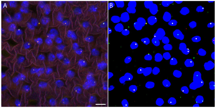 Figure 1
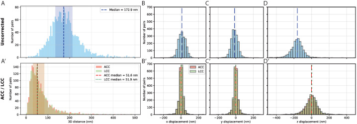 Figure 2
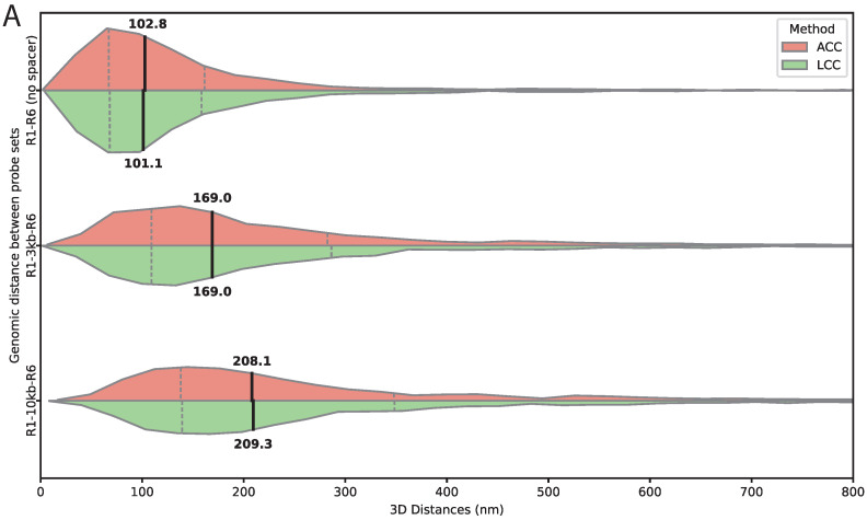 Figure 3
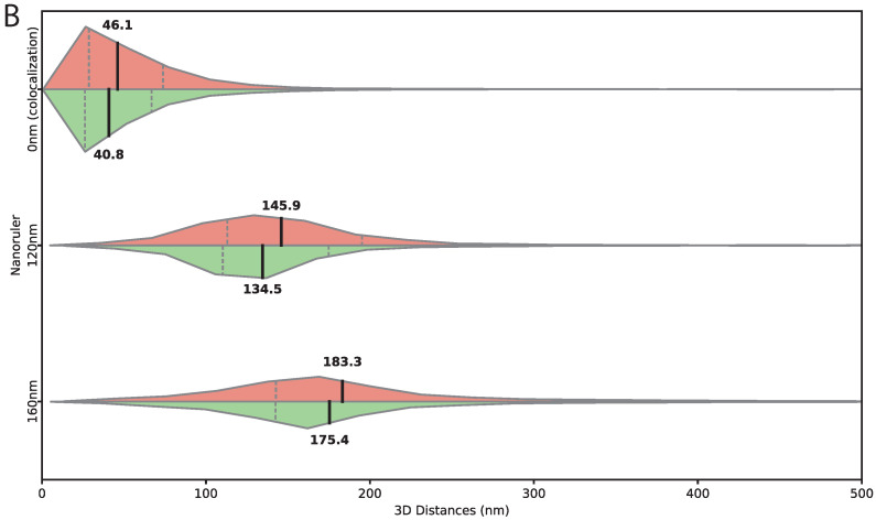 Figure 4
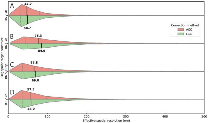 Figure 5
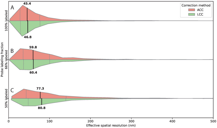 Figure 6
- —Fondation pour la Recherche Médicale
- —ANR
- —France 2030 programme
Peer Reviews
No public reviews on file for this paper yet. If you reviewed it on a platform where reviews are public (OpenReview, ICLR, NeurIPS, ICML), you can paste yours below so the community can read it here.
Videos
No videos yet. Explain this paper in a talk, walkthrough, or lecture? Add one.
Taxonomy
TopicsGenomics and Chromatin Dynamics · Single-cell and spatial transcriptomics · Advanced Fluorescence Microscopy Techniques
1. Introduction
The three-dimensional organization of the genome is fundamental to gene regulation [1], as spatial proximity between regulatory elements and their target genes directly influences transcription [2,3]. Fluorescence in situ hybridization (FISH), including modern Oligopaint-based approaches, remains a gold-standard method for visualizing these spatial relationships with single-cell resolution within the native nuclear context [4,5,6,7].
While existing FISH studies and computational tools, sometimes complemented by Hi-C-based maps, have significantly advanced our understanding of large-scale chromosomal structures and long-range interactions spanning hundreds of kilobases to megabases [6,8,9,10,11,12,13], many critical regulatory interactions—such as enhancer–promoter loops and local chromatin contacts—occur at much finer genomic scales (<10–100 kb) [14]. At these scales, technical limitations, including chromatic aberration, can introduce measurement errors that are comparable to, or even exceed, the biological distances being investigated.
Despite the biological significance of short-range genomic measurements, many studies still rely on user-dependent distance measurements, which are prone to error [15,16,17,18]. Existing computational tools are typically not designed or rigorously validated for high-precision quantification at these scales. Moreover, the relationship between FISH probe design parameters—such as probe density and target sequence length—and measurement accuracy remains poorly characterized for short-distance applications.
Here we present FISH-Dist, an automated computational pipeline for quantitative 3D distance measurements in FISH imaging, with a focus on short-range genomic distances. FISH-Dist integrates deep learning-based spot detection [19], sub-pixel 3D Gaussian fitting, and complementary chromatic aberration correction strategies for high-resolution measurements. We validate the pipeline using orthogonal approaches, including colocalization experiments and calibrated nanorulers. Using FISH-Dist, we also systematically quantify how probe design parameters, such as labeling density and target sequence length, influence measurement accuracy, providing practical guidance for experimental planning. By addressing technical limitations in standard confocal FISH, FISH-Dist provides a reproducible framework for quantifying spatial relationships at the short genomic distances most relevant to gene regulation.
2. Materials and Methods
2.1. Oligopaint Probe Synthesis
Forty-five-nucleotide single-stranded DNA Oligopaint probes targeting specific DNA sequences were designed by Daicel Arbor Biosciences and synthesized from myTags Immortal Libraries (Daicel Arbor Biosciences, Ann Arbor, MI, USA) according to the manufacturer’s protocol [20]. Briefly, myTags Immortal Libraries were amplified by PCR, and the resulting products were column-purified. In vitro transcription was then performed to generate RNA, which was column-purified and used as a template for reverse transcription (RT). When RNA concentration was insufficient for RT, an additional ethanol precipitation was performed. RT was carried out using fluorescent primers (coupled at the 5′ end with a single ATTO 565 or ATTO 633 fluorescent dye) purchased from Integrated DNA Technologies (Coralville, IA, USA). Unincorporated primers were degraded, and RNA:DNA hybrids were column-purified. RNA fragments were subsequently removed by RNAse treatment, and the resulting fluorescent single-stranded DNA probes were column-purified and stored at −20 °C. The fraction of successfully dye-conjugated probes was quantified using a Nanodrop spectrophotometer (Thermo Fisher Scientific, Waltham, MA, USA) to ensure an appropriate labeling ratio. Detailed sequences for all oligos are available in Supplementary File S1.
2.2. Oligopaint Probe Design for Spatial Resolution Calibration in Multi-Color FISH
Oligopaint probes were designed to target a ∼10 kb endogenous genomic region (X:6,760,094–6,770,369, Drosophila genome Release 6) adjacent to the attP18 landing site on the X chromosome of Drosophila melanogaster. A total of 142 Oligopaint probes were designed to hybridize exclusively to the + DNA strand of this locus. For dual-color experiments, the same probe set was labeled with either ATTO 565 or ATTO 633 fluorophores.
2.3. Construction and Oligopaint Targeting of Synthetic Reporter Sequences
Two synthetic reporter sequences (R1 and R6) were designed to be orthogonal to the Drosophila melanogaster genome by Daicel Arbor Biosciences and synthesized by Genewiz. Each reporter consists of a 2 kb DNA sequence absent from the D. melanogaster genome, with similar overall GC content but distinct sequence composition. Each reporter was targeted by a set of 87 Oligopaint probes tiled across the entire sequence and both DNA strands. Transgenes were integrated at the ZH-2A landing site on the X chromosome using site-specific recombination. Detailed sequences for all oligos are available in Supplementary File S1.
2.4. Transgene Design for Defined 3D Genomic Distance Measurements
To evaluate the accuracy of 3D distance measurements under biological conditions, we generated transgenic constructs containing two distinct Oligopaint-tagged sets targeting R1 and R6, labeled with ATTO 565 and ATTO 633 and separated by defined spacer lengths of 0 kb, 3 kb, or 10 kb. In all constructs, the spacer is flanked on both sides by the synthetic reporter tags R1 and R6, which serve as independent Oligopaint target sites. 3kb spacer consists of randomly generated DNA sequences designed to minimize binding of known Drosophila transcription factors. The 10 kb spacer is a cherry-tagged yellow gene of Drosophila biarmipes. All constructs were integrated at the ZH-2A landing site. Detailed sequences for all constructs are available in Supplementary File S1.
2.5. Oligopaint Target Length Variants for Assessing Spatial Resolution
To examine how FISH target sequence length influences spatial resolution, a series of transgenic constructs was generated in which progressively shorter segments of the R6 synthetic reporter were used as Oligopaint targets. Three target lengths were tested—2 kb, 1 kb, and 500 bp—preserving sequence composition while varying target size. All constructs were integrated at the ZH-2A landing site, ensuring a constant genomic context across conditions.
2.6. Modulation of Oligopaint Probe Density
To assess the impact of Oligopaint probe density on measurement performance, the fraction of fluorescently labeled probes targeting a fixed 2 kb R6 genomic region was systematically varied while maintaining a constant total probe concentration. This was achieved by mixing fluorescently labeled probes with unlabeled (“cold”) probes targeting the same sequence, thereby preserving hybridization conditions while progressively reducing the number of fluorescent probes contributing to the detected signal.
Three labeling conditions were examined. In the fully labeled condition (∼100%), the 2 kb R6 locus could be covered by up to 87 labeled probes and no unlabeled probes; ATTO 565- and ATTO 633-labeled probe sets were each used at a final concentration of 3 ng/µL, resulting in a total labeled probe concentration of 6 ng/µL. In the intermediate labeling condition (∼66%), the locus could be covered by up to 57 labeled probes and 30 unlabeled probes; each labeled probe set was used at 2 ng/µL and supplemented with 2 ng/µL of unlabeled probes. In the lowest labeling condition (∼50%), the locus could be covered by up to 43 labeled probes and 43 unlabeled probes; here, each labeled probe set was used at 1.5 ng/µL and supplemented with 3 ng/µL of unlabeled probes. In all cases, the total probe concentration was maintained at 6 ng/µL. Hybridization, imaging, and signal detection were performed under standard conditions.
2.7. Fluorescence In Situ Hybridization on Late Pupal Wings
At 70 h after puparium formation (APF), male flies -carrying a single X chromosome, and therefore a single set of each probe- were immobilized on adhesive tape, removed from their pupal cases, and gently dragged across the tape surface to remove residual cuticle shed during pupal development. Specimens were transferred to a small dish containing deionized water for approximately 1 min to allow wing unfolding. Wings were fixed in 4% formaldehyde in PBTT (1× PBS, 0.1% Tween-20, 0.3% Triton X-100) for 30 min at room temperature (RT), then washed twice in PBS. At 70 h APF, wings are enclosed by non-permeable cuticle and therefore require mechanical separation of the dorsal and ventral epithelial layers prior to probe hybridization. To achieve this, wings were transferred in a droplet of deionized water onto a non-adhesive substrate, typically the protective liner of double-sided tape. Excess water was removed, and wings were arranged flat without overlap. A strip of Tesa ECO & ULTRA tape (66 m × 50 mm)—selected for minimal autofluorescence, as it remains attached throughout subsequent staining, mounting, and imaging steps—was gently pressed onto the wings and lifted, ensuring wing adhesion to the tape. The taped wings were overlaid with a second tape strip and pressed gently to preserve structural integrity. The two tape layers were then carefully separated, thereby splitting the dorsal and ventral wing epithelial layers. Finally, the separated wing layers, still tape-mounted, were post-fixed for 20 min at RT in 4% formaldehyde in PBTT.
Wings were then briefly rinsed twice by rapid addition and removal of 500 µL freshly prepared PBS with 0.1% Tween-20 (PTw), followed by two 10 min washes in the same buffer. Wings were incubated for 1 h at 37 °C with RNase A diluted at 1:100 in PTw, then transferred to a 0.05 M HCl solution for 5 min to denature DNA and enhance probe penetration.
Wings were washed sequentially for 15 min each in 4:1, 1:1, 1:4, and 0:1 mixtures of PTw and FISH wash buffer (Fwb; 35% formamide, 0.1% Tween-20, 4X SSC). Fwb was prepared fresh before use and stored at 4 °C for a maximum of 48 h.
Wings were incubated with probes diluted to a final concentration of 3 ng/µL each in hybridization buffer (50% formamide, 5X SSC, 0.1% Tween-20, 100 µg/mL denatured herring sperm DNA, 50 µg/mL heparin). The samples were heated at 87 °C for 20 min in a thermocycler, then cooled gradually to 37 °C over 2 h. Hybridization was performed overnight for 12–16 h at 37 °C.
Following hybridization, wings were rinsed briefly, then washed twice for 1 h each at 37 °C in pre-warmed Fwb. Nuclei were stained with 20 mM Hoechst diluted 1:500 in PTw for 5 min, followed by four 10 min washes in PTw at RT. Wings were mounted in Vectashield, flattened under a coverslip using gentle pressure applied with magnets, and sealed with nail polish.
2.8. Nanorulers Calibration Standards
DNA origami nanorulers (GATTAquant GmbH, Munich, Germany) were employed as ground truth standards for validation of distance measurements [21]. These nanostructures consist of self-assembled DNA origami scaffolds with precisely positioned fluorescent dye attachment sites labeled with 40 ATTO 565 and 40 ATTO 633. Nanorulers with defined inter-dye separations of 120 nm and 160 nm were used to assess distance measurement accuracy, while a design with intermingled 40 ATTO 565 and 40 ATTO 633 dyes, effectively representing zero separation, served as a colocalization standard to evaluate measurement precision. Mounted slides were provided directly by the manufacturer. For each nanoruler type, images were acquired under conditions identical to those used for Drosophila wing samples.
2.9. Confocal Imaging
Hoechst, ATTO 565, and ATTO 633 channels were acquired on a Zeiss LSM 780 confocal microscope (Carl Zeiss Microscopy GmbH, Jena, Germany) using a Plan-Apochromat 40× oil immersion objective (NA 1.4). To minimize inter-channel displacement, line switching mode was employed instead of frame switching. Images were acquired with laser power of 0.2% (405 nm), 15% (565 nm), and 27% (633 nm); dwell time of 1.57 µs; voxel size of 103.8 nm × 103.8 nm × 250 nm; 16-bit depth. The pinhole was set to 1 Airy unit (AU) for the 488 nm wavelength.
2.10. Deep Learning-Based Detection of Nuclei and Spots
Nuclei and Oligopaint spots were detected using two independently trained deep learning models [19] applied to individual 2D planes of 3D image stacks, producing volumetric segmentations. Models were trained using EPySeg [22], with data augmentation (rotations, flips, intensity scaling). Probabilistic output maps were thresholded to yield binary masks for nuclei and point coordinates for spots.
2.11. Subpixel 3D Spot Centroid Extraction via Gaussian Fitting
Subpixel 3D coordinates of detected spots were refined using the Big-FISH Python library [23], providing initial coordinates and estimated spot sizes for a 3D Gaussian fit. This procedure yielded precise centroids even in the presence of moderate background noise.
2.12. Spot Pairing Across Channels
Before applying chromatic aberration correction, corresponding Oligopaint spots were paired across channels based on spatial proximity. For each image, detected 3D spot coordinates were used to identify the nearest neighbor in the other channel. When applicable, only spots located within segmented nuclei were considered for pairing, thereby excluding non-genomic or non-specific signals. The resulting paired centroids serve as the input for chromatic aberration corrections.
2.13. Linear Chromatic Correction (LCC)
To correct for chromatic aberrations and ensure unbiased distance measurements, we applied a method we named the Linear Chromatic Correction [14,24,25]. The principle underlying this correction is that, for paired FISH Oligopaint centroids, the mean difference between corresponding points should be zero in the absence of chromatic aberration—the pairs should have no preferred orientation—regardless of whether the points are colocalized or distant [14,24].
The correction procedure begins by computing the difference between each pair of centroids. The mean of these differences is subtracted to center the distribution at zero. For each spatial axis, a linear regression model is fitted to estimate the scaling bias. One set of points is then corrected using these per-axis scaling factors. Finally, any residual global translation is removed to ensure that the corrected differences remain centered at zero.
2.14. Affine Chromatic Correction (ACC)
In addition to LCC, we implemented an independent global method to correct chromatic aberrations by aligning spot coordinates across channels using a 3D affine transformation. This approach compensates for systematic inter-channel discrepancies, including global translations, anisotropic scaling, rotations, and shear.
The procedure operates on paired, colocalized Oligopaint centroids extracted from multiple images sharing the same chromatic aberration profile, acquired on the same microscope within a limited time window. To reduce the influence of mismatched pairs, pairwise distances are filtered using the median and interquartile range (IQR), removing extreme outliers that could strongly bias the affine transformation. Filtered paired centroids from all images are then aggregated to estimate a single global affine transformation matrix.
The affine transformation is estimated by minimizing the squared displacement between corresponding points, allowing for translation, rotation, anisotropic scaling, and shear. The transformation matrix is computed using an implementation adapted from a library by C. Gohlke [26], which solves the resulting least-squares point-set alignment problem using a singular value decomposition (SVD)-based approach. Once estimated, the transformation is applied to all points in one channel to generate corrected coordinates.
The resulting affine transform is stored and can be reapplied to images of non-colocalized spots acquired under the same conditions and within short time intervals, allowing consistent correction across datasets.
2.15. Distance Measurements and Resolution Assessment
Euclidean distances between registered, colocalized spots were calculated in 3D to assess spatial resolution. Distances for non-colocalized spots were similarly computed to quantify inter-locus spacing. Distributions were visualized using histograms and violin plots in Matplotlib (version 3.10.8) and Seaborn (version 0.13.2) [27,28], and robust statistics (median and interquartile range, IQR) were used to limit the influence of outliers and assess chromatic correction precision and spatial organization.
3. Results
3.1. Quantifying and Correcting Chromatic Aberration to Establish the Baseline Resolution
To establish the baseline resolution of our imaging system and quantify the impact of chromatic aberration on distance measurements, we performed colocalization experiments in which the same ∼10 kb endogenous genomic region adjacent to the attP18 landing site was labeled with two distinct fluorophores using Oligopaint probes (Figure 1; see Section 2). Because both probe sets target the identical locus, any observed separation reflects technical artifacts rather than true biological distances.
Analysis of 1917 dual-labeled spots revealed substantial systematic offsets between channels before chromatic aberration correction (Figure 2A). The distribution of measured distances showed a median value of 172.9 nm (IQR = 135.2–212.3 nm), with some spot pairs exhibiting apparent separations exceeding 500 nm. Chromatic aberration was highly anisotropic: lateral (XY) components showed median offsets of 29.7 nm in x and 27.3 nm in y (Figure 2B,C), whereas the axial (Z) component exhibited a median offset of 162.5 nm (Figure 2D). This reflects wavelength-dependent refractive index effects and the lower axial resolution of confocal microscopy.
Application of chromatic aberration correction substantially reduced inter-channel distances. Both the affine (ACC) and linear (LCC) correction methods decreased the median 3D distance from 172.9 nm (uncorrected) to 51.6 nm (IQR: 32.2–82.9 nm) for ACC and 51.9 nm (IQR: 32.2–82.7 nm) for LCC, indicating a marked reduction in systematic offsets (Compare Figure 2A and Figure 2A′). Component-wise median displacements after correction were similar between methods: 12.8–13.1 nm in x, 13.6–13.7 nm in y, and 39.7–40.5 nm in z (Figure 2B′–D′). This close agreement confirms both methods accurately model chromatic aberration. Residual distances likely reflect localization uncertainty, probe accessibility differences, and stochastic variation in probe positioning.
Analysis of residual chromatic displacements after affine correction revealed no obvious position-dependent variation (Figure S1A,B), indicating that the global correction captures the majority of systematic offsets. Decomposition of the 3D displacement vectors confirmed strong anisotropy, with lateral (XY) components showing no preferential in-plane orientation bias, whereas the axial (Z) component dominated (Figure S1C). The consistent agreement between correction methods throughout subsequent experiments further provides internal validation of measurement accuracy.
3.2. Validation of 3D Distance Measurements Using Genomic Standards and DNA Origami Nanorulers
To evaluate the accuracy of 3D distance measurements under biological conditions, we used a transgene containing two Oligopaint target sites, R1 and R6, labeled with ATTO 565 and ATTO 633, separated by 0 kb, 3 kb, or 10 kb spacers. Chromatic aberrations in these images were corrected using an affine transformation derived from a parallel colocalization experiment acquired under identical imaging conditions. After correction, the measured 3D distances between the two labeled regions increased systematically with spacer length (Figure 3A). For the 0 kb spacer, median distances were 102.8 nm and 101.1 nm for the ACC and LCC methods, respectively. For the 3 kb spacer, median distances increased to 169.0 nm with both methods, and for the 10 kb spacer, they reached 208.1 nm and 209.3 nm.
While the dual-targeted transgene provides qualitative insight into chromatic aberration and distance measurement precision, definitive ground-truth validation of absolute distances was achieved using GATTAquant DNA origami nanorulers [21]. Three types of nanorulers were employed, including one with intermixed ATTO 565 and ATTO 633 fluorophores suitable for registration and resolution assessment, and two with fixed inter-fluorophore separations of 120 nm and 160 nm. For each nanoruler type, we imaged over 4000 individual structures and measured 3D distances after chromatic aberration correction using both ACC and LCC methods. Due to technical constraints, calibration could not be performed using the intermixed nanoruler; instead, registration was derived from dual-color colocalization experiments on wing samples.
For the intermixed nanoruler, the median measured 3D distance was 40.8 nm (IQR: 26.2–66.8 nm) using LCC and 46.1 nm (IQR: 28.6–73.8 nm) using ACC (Figure 3B). For the 120 nm nanoruler, LCC yielded a median distance of 134.5 nm (IQR: 110.3–174.8 nm), while ACC measured 145.9 nm (IQR: 113.1–195.2 nm). For the 160 nm nanoruler, LCC produced a median distance of 175.4 nm (IQR: 142.5–304.8 nm), with ACC yielding 183.3 nm (IQR: 142.7–335.1 nm) (Figure 3B). Both correction approaches accurately reproduced expected distances—and distance differences—across nanoruler sizes, confirming the reliability of the measurements.
3.3. Target Sequence Length and Composition Affect Spatial Resolution
To assess how target sequence length—at constant probe density—affects resolution, we used transgenes containing the full 2 kb R6 region and truncated versions of 1 kb and 500 bp, co-labeled with ATTO 565 and ATTO 633. For the 2 kb construct, median residual distances were 47.7–48.7 nm (Figure 4A). The 1 kb construct showed substantially increased distances of 76.3–84.9 nm (Figure 4B), while the 500 bp construct yielded 65.8–69.0 nm (Figure 4C).
Target length strongly affected detection yield. Average detected spots per image decreased from 190.5 spots (2kb) to 57.4 (1 kb) and 34.0 (500 bp) (Table 1), reflecting reduced probe binding sites and signal intensity.
To assess whether factors other than target length contribute to measurement performance, we analyzed an additional 2 kb construct, R1, inserted at the same genomic locus but exhibiting a different DNA sequence compared to R6. Importantly, this construct was targeted by the same number of Oligopaint probes as the original 2 kb construct, ensuring comparable probe density and labeling strategy. Despite these similarities, the alternative sequence yielded fewer detected pairs per image (128.8 versus 190.5, Table 1) and slightly larger residual inter-channel distances (compare Figure 4A and Figure 4D). This indicates that sequence-dependent effects—potentially related to hybridization efficiency or local chromatin organization—can modulate measurement performance even when target length and probe number are constant.
3.4. Probe Density Influences Detection Efficiency and Spatial Resolution
To evaluate the impact of probe density on measurement performance, we systematically varied the fraction of fluorescently labeled Oligopaint probes targeting a fixed 2 kb genomic region by adjusting the ratio of labeled to unlabeled probes while keeping the total probe mass constant. This approach preserves hybridization conditions while progressively reducing the number of fluorescent probes contributing to the detected signal.
Three labeling conditions were examined, corresponding to approximately 100%, 66%, and 50% fluorescent labeling. Under these conditions, the 2 kb R6 locus could be covered by up to 87, 57, or 43 fluorescently labeled Oligopaint probes, with the remainder of the locus filled by 0, 30, or 43 unlabeled Oligopaint probes. Fully labeled conditions yielded an average of 190.5 spots per image (Table 2). Reducing the labeled fraction to ∼66% decreased detection to 133.2 spots per image, and further reducing it to ∼50% resulted in only 51.1 spots per image (Table 2). Reducing the fraction of labeled probes lowers fluorescence signal, diminishing both detection efficiency and localization precision, highlighting the strong dependence of measurement performance on the number of fluorescent probes present.
Spatial resolution also worsened with decreasing labeling fraction, although less sharply than detection efficiency. After affine chromatic aberration correction, the median residual distance increased from 45.4 nm at 100% labeling to 59.8 nm at ∼66% labeling and 77.3 nm at ∼50% labeling (Figure 5). Comparable values were obtained using linear chromatic aberration correction, with median residual distances of 46.8 nm, 60.4 nm, and 80.8 nm, respectively (Figure 5), demonstrating that this trend is robust across correction methods.
4. Discussion
4.1. FISH-Dist Enables Reproducible 3D Measurements of Short-Range Genomic Distances
We developed FISH-Dist, an automated pipeline designed for quantitative 3D distance measurements in FISH imaging at the kilobase scale. FISH-Dist combines deep learning-based spot detection, sub-pixel 3D localization, and dual chromatic aberration correction methods (affine and linear), with performance assessed using calibrated standards such as DNA origami nanorulers.
While many existing FISH tools focus on large-scale chromosomal structures (hundreds of nanometers to micrometers), biologically critical interactions—such as enhancer–promoter contacts, local chromatin loops, regulatory clustering within topologically associating domains, DNA damage foci, and homologous chromosome pairing—occur at much shorter distances (10–50 kb). At these scales, chromatic aberration and localization precision are limiting factors. In our system, uncorrected inter-channel offsets exceeded 170 nm, with axial components approaching 160 nm—comparable to or larger than many true biological separations. FISH-Dist reduces these errors to approximately 50 nm for colocalized targets.
Additionally, we demonstrate that 2 kb probe targets offer an optimal balance between detection efficiency and spatial compactness, achieving ∼45 nm resolution. These advances enable robust, quantitative measurement of short-range genomic interactions that are typically inaccessible to conventional FISH analysis pipelines.
4.2. Probe Design Guidelines Emerge from Systematic Parameter Testing
Our systematic evaluation of probe design parameters yielded several actionable insights for experimental optimization. The relationship between target sequence length and resolution reveals a critical trade-off: longer sequences improve detection efficiency but compromise localization precision. Our 2 kb construct achieved optimal 45 nm resolution with robust detection (190.5 spots/image). Shortening to 1 kb degraded resolution to 75–80 nm despite reduced target size. The 500 bp construct showed slightly better resolution (∼70 nm) than 1 kb but both exhibited markedly reduced detection efficiency.
These findings indicate that competing effects exist, with shorter targets providing compact labeling but reduced signal intensity and fewer probe binding sites, both of which compromise localization. The 2 kb length represents a favorable compromise. Importantly, sequence composition influences performance even at fixed length, as the R1 construct showed reduced efficiency despite having the same length and number of probes as R6. Factors such as GC content, secondary structure, or chromatin accessibility likely modulate hybridization efficiency.
Probe density experiments showed reducing labeling from 100% to 66% caused moderate degradation (45 nm to 60 nm resolution, 30% detection loss). Further reduction to 50% caused substantial degradation (80 nm resolution, 75% detection loss). Even with probe excess, reducing fluorescent fraction diminishes photon counts, degrading centroid localization. For high spatial accuracy, we recommend maintaining at least 57 oligos/fluorphores per probe set spanning 2 kb (corresponding to labeling in our conditions).
Our optimization was conducted in specific genomic and cellular contexts. Absolute values likely depend on chromatin accessibility, nuclear architecture, and cell type. However, general principles—optimal target length balancing signal and compactness, sequence-dependent performance, sensitivity to probe density—should apply broadly. We encourage pilot optimization in specific biological systems.
4.3. Methodological Considerations and Limitations
Validation with DNA origami nanorulers provides ground-truth accuracy under idealized conditions, while transgene-based measurements in fixed biological samples demonstrate accuracy in realistic contexts where chromatin organization and nuclear architecture are preserved. This combination represents a strength of our approach, as it bridges artificial calibration standards and biologically relevant measurements. Nevertheless, probe accessibility can vary with chromatin state, DNA sequence, and cell cycle stage. Although fixation stabilizes chromatin structure, labeled DNA retains conformational heterogeneity reflecting the ensemble of chromatin configurations present at fixation, such that measured distances represent spatial averages rather than rigid, single conformations.
Our chromatic aberration correction assumes a stable optical transformation between channels during image acquisition, and performance may degrade in samples with substantial axial drift or stage movement. In addition, the deep learning-based spot detection relies on training data representative of the target application. Although the trained model generalizes well across the range of probes, labeling densities, and imaging conditions tested here, users working with substantially different probe types or imaging modalities may benefit from retraining or fine-tuning the model. Due to their size, the training datasets and scripts are not publicly distributed but are available upon request.
Throughout validation and optimization, we employed two conceptually distinct chromatic aberration correction approaches, affine and linear, which consistently produced nearly identical corrected distances across all tested conditions, typically differing by only a few nanometers. This close agreement indicates that both methods accurately model the chromatic aberration in our imaging system and provides an internal consistency check that strengthens confidence in measurements.
Although the two approaches differ primarily in workflow rather than performance, maintaining both in the analysis pipeline offers important diagnostic value. Agreement between methods, as observed here, confirms optical stability and the adequacy of global correction models, whereas substantial divergence would indicate optical instability or model inadequacy and prompt re-evaluation of imaging conditions. Consistent with this interpretation, spatial analysis of residual displacements revealed relatively uniform chromatic aberration fields across the imaging volume, indicating that global correction models capture most systematic offsets in our system. Users are nevertheless encouraged to assess spatial uniformity in their own setups to determine the most appropriate correction strategy.
4.4. Comparison with Existing Methods
Several computational tools exist for FISH image analysis, each with distinct design priorities and validation strategies. Classical approaches based on watershed segmentation or intensity thresholding remain widely used, but they often require manual parameter tuning or segmentation, which is error-prone and can lead to substantial over-segmentation, particularly under variable background conditions or in regions with densely packed spots.
Particle tracking frameworks such as TrackMate [29] provide flexible and sophisticated spot detection and localization, capable of handling multiple spots per frame. Tools like the DNA-FISH Fiji plugin [30], which leverages TrackMate for spot detection, offer semi-automated analysis of FISH images, including distance measurements between genomic loci. However, in noisy images such as ours, these methods can generate excessive false-positive detections. While post-processing can mitigate this, the procedure is often slow and not optimized for high-throughput FISH distance measurements. Additionally, neither TrackMate nor the DNA-FISH plugin explicitly addresses chromatic aberration correction, which is critical for accurate short-range distance quantification.
FISH-quant [23] is the most directly comparable tool. However, it was developed primarily for RNA FISH and transcript quantification rather than precise genomic distance measurements and does not include chromatic aberration correction. In contrast, FISH-Dist is specifically designed for short-range genomic distances, implements two complementary chromatic aberration correction methods (linear and affine), and has been rigorously validated using both transgenic constructs and DNA origami nanorulers. Its systematic evaluation of probe design parameters provides increased confidence in quantitative accuracy compared with single-method or less extensively validated pipelines.
5. Conclusions
FISH-Dist has been developed with accessibility and reproducibility in mind. The complete analysis pipeline is available as open-source software, accompanied by comprehensive documentation, example datasets, and tutorials to facilitate adoption. The tool is provided as a command-line application and includes pre-trained deep learning models that support many standard use cases, while also allowing retraining or fine-tuning for specialized experimental conditions.
More broadly, FISH-Dist provides a validated and automated framework for quantitative 3D distance measurements in genome organization studies. By integrating chromatic aberration correction, robust spot detection, and systematic distance analysis into a single workflow, the pipeline reduces technical barriers and enables reproducible, high-throughput spatial measurements across diverse experimental systems.
The reference list from the paper itself. Each links out to its DOI / PubMed record.
- 1Dixon J.R. Selvaraj S. Yue F. Kim A. Li Y. Shen Y. Hu M. Liu J.S. Ren B. Topological domains in mammalian genomes identified by analysis of chromatin interactions Nature 201248537638010.1038/nature 1108222495300 PMC 3356448 · doi ↗ · pubmed ↗
- 2Popay T.M. Dixon J.R. Coming Full Circle: On the Origin and Evolution of the Looping Model for Enhancer–Promoter Communication J. Biol. Chem.202229810.1016/j.jbc.2022.102117 PMC 928393935691341 · doi ↗ · pubmed ↗
- 3Kim S. Shendure J. Mechanisms of Interplay between Transcription Factors and the 3D Genome Mol. Cell 20197630631910.1016/j.molcel.2019.08.01031521504 · doi ↗ · pubmed ↗
- 4Beliveau B.J. Boettiger A.N. Avendaño M.S. Jungmann R. Mc Cole R.B. Joyce E.F. Kim-Kiselak C. Bantignies F. Fonseka C.Y. Erceg J. Single-molecule super-resolution imaging of chromosomes and in situ haplotype visualization using Oligopaint FISH probes Nat. Commun.20156714710.1038/ncomms 814725962338 PMC 4430122 · doi ↗ · pubmed ↗
- 5Beliveau B.J. Joyce E.F. Apostolopoulos N. Yilmaz F. Fonseka C.Y. Mc Cole R.B. Chang Y. Li J.B. Senaratne T.N. Williams B.R. Versatile design and synthesis platform for visualizing genomes with Oligopaint FISH probes Proc. Natl. Acad. Sci. USA 2012109213012130610.1073/pnas.121381811023236188 PMC 3535588 · doi ↗ · pubmed ↗
- 6Bolzer A. Kreth G. Solovei I. Koehler D. Saracoglu K. Fauth C. Müller S. Eils R. Cremer C. Speicher M.R. Three-Dimensional Maps of All Chromosomes in Human Male Fibroblast Nuclei and Prometaphase Rosettes P Lo S Biol.20053 e 15710.1371/journal.pbio.003015715839726 PMC 1084335 · doi ↗ · pubmed ↗
- 7Fields B.D. Nguyen S.C. Nir G. Kennedy S. A multiplexed DNA FISH strategy for assessing genome architecture in Caenorhabditis eleganse Life 20198 e 4282310.7554/e Life.4282331084706 PMC 6516958 · doi ↗ · pubmed ↗
- 8Shirley J.W. Ty S. Takebayashi S.i. Liu X. Gilbert D.M. FISH Finder: A high-throughput tool for analyzing FISH images Bioinformatics 20112793393810.1093/bioinformatics/btr 05321310746 PMC 3065689 · doi ↗ · pubmed ↗