Model-independent searches of new physics in DARWIN with deep learning
J. Aalbers, J. Aalbers, K. Abe, M. Adrover, S. Ahmed Maouloud, L. Althueser, D. W. P. Amaral, B. Andrieu, E. Angelino, D. Antón Martin, B. Antunovic, E. Aprile, M. Babicz, D. Bajpai, M. Balzer, E. Barberio, L. Baudis, M. Bazyk, N. F. Bell, L. Bellagamba, R. Biondi, Y. Biondi

TL;DR
This paper introduces a deep learning method to detect anomalies in the DARWIN experiment without assuming specific models of dark matter.
Contribution
A model-independent, likelihood-free deep learning pipeline for anomaly detection in direct dark matter experiments.
Findings
The method uses a VAE and classifier to learn event features from high-dimensional data.
It achieves high accuracy while reducing analysis time and reliance on traditional cuts.
The approach is validated using simulated WIMP dark matter signals.
Abstract
We present a deep learning pipeline to perform a model-independent, likelihood-free search for anomalous (i.e., non-background) events in the proposed next-generation multi-ton scale liquid xenon-based direct detection experiment, DARWIN. We train an anomaly detector comprising a variational autoencoder (VAE) and a classifier on high-dimensional simulated detector response data and construct a 1D anomaly score to reject the background-only hypothesis in the presence of an excess of non-background-like events. We use simulated validation data to determine the power of the method to reject the background-only hypothesis in the presence of a WIMP dark matter signal, without any model-dependent assumption about the nature of the signal. We show that our neural networks learn relevant features of the events from low-level, high-dimensional detector outputs, avoiding lossy and computationally…
Genes, proteins, chemicals, diseases, species, mutations and cell lines named across the full text — each resolved to its canonical identifier and authoritative record.
Click any figure to enlarge with its caption.
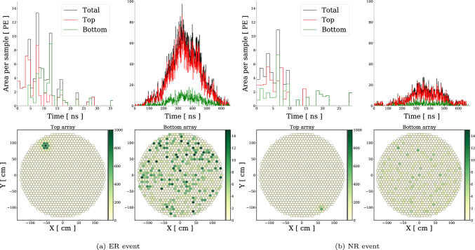 Figure 1
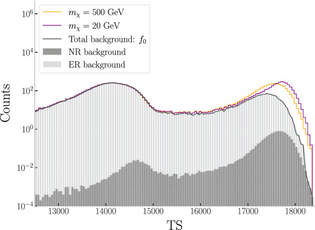 Figure 2
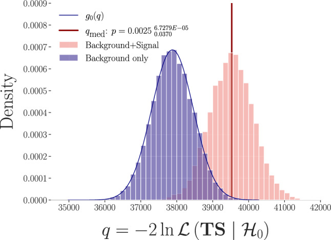 Figure 3
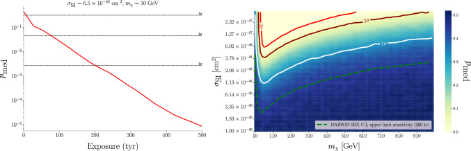 Figure 4
 Figure 5
 Figure 6
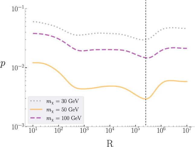 Figure 7
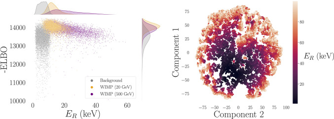 Figure 8
 Figure 9
- —US National Science Foundation (NSF)
- —Dutch Science Council
- —http://dx.doi.org/10.13039/100010663H2020 European Research Council
- —Fondazione ICSC, Spoke 3 “Astrophysics and Cosmos Observations”, Piano Nazionale di Ripresa e Resilienza Project ID CN00000013 “Italian Research Center on High-Performance Computing, Big Data and Quan
- —http://dx.doi.org/10.13039/501100004189Max-Planck-Gesellschaft
- —PortugueseFCT
- —http://dx.doi.org/10.13039/501100000271Science and Technology Facilities Council
- —Ministry of Education, Science and Technological Development of the Republic of Serbia
- —http://dx.doi.org/10.13039/100018694HORIZON EUROPE Marie Sklodowska-Curie Actions
- —http://dx.doi.org/10.13039/100031478NextGenerationEU
- —http://dx.doi.org/10.13039/501100001711Schweizerischer Nationalfonds zur Förderung der Wissenschaftlichen Forschung
- —DS4ASTRO: Data Science methods for Multi-Messenger Astrophysics & Multi-Survey Cosmology”, in the framework of the PRO3 ‘Programma Congiunto’ of the Italian Ministry for University and Research
Peer Reviews
No public reviews on file for this paper yet. If you reviewed it on a platform where reviews are public (OpenReview, ICLR, NeurIPS, ICML), you can paste yours below so the community can read it here.
Videos
No videos yet. Explain this paper in a talk, walkthrough, or lecture? Add one.
Taxonomy
TopicsDark Matter and Cosmic Phenomena · Particle physics theoretical and experimental studies · Computational Physics and Python Applications
Introduction
A promising method for investigations of the ever-elusive dark matter sector involves seeking excess nuclear recoils in subterranean detectors, a strategy known as direct detection (DD) [1]. Over the years, a number of xenon (XENONnT [2], LUX-ZEPLIN (LZ) [3], PandaX[4]) and argon (DEAP-3600 [5], DarkSide-20k [6], ArDM [7]) ton-scale experiments have steadily enhanced the sensitivity to physics beyond the standard model (BSM), and this effort is expected to continue, with plans for a next-generation dark matter and neutrino observatory. While earlier designs for a ‘dark matter WIMP search with liquid xenon’ observatory (DARWIN) [8, 9] aimed at an active liquid xenon target mass of 40 tons, the recently formed XLZD Collaboration proposes an even more ambitious target mass of 60–80 tons [10]. While the design of the XLZD experiment is being developed, this paper focuses on DARWIN, a well-defined proposal for a large-scale observatory using a xenon dual-phase time projection chamber (TPC) to study phenomena requiring low-background conditions. DARWIN aims to be sensitive to weakly interacting massive particle (WIMP) dark matter as well as neutrinoless double beta decay, axion-like particles, and any other BSM particles that would manifest through significant interaction with a xenon target. The aim of this work is to introduce a signal model-agnostic, deep learning-based analysis pipeline, offering a complementary and alternative approach to the standard likelihood-based analysis chain in such a detector. The benefits of this approach are that it enables a fuller exploitation of the detector readout data, without the information loss potentially incurred in using only hand-crafted summary statistics (such as cS1 and cS2, the corrected prompt primary scintillation and secondary electroluminescence of ionized electrons signals, respectively), and that it can include in the pipeline any physics effect that can be faithfully simulated, including systematics.
Machine learning (ML) has emerged as a powerful tool within the physics community, and its relevance to DM phenomenology has been growing rapidly [11–15].
Unsupervised machine learning has been increasingly employed in collider physics to identify anomalies in data, as demonstrated in several recent studies [16–27], with early example applications on simulated events of CMS and ATLAS already in Refs. [28, 29], as well as Ref. [30], where an “anomaly awareness” algorithm is proposed. ML techniques were also applied to DD experiments for a variety of tasks, ranging from signal classification to fast likelihood evaluation [31–36]. Ref. [32] utilizes a semi-unsupervised deep neural network comprising a pretrained convolutional neural network (CNN) and a VAE in order to detect the presence of excess nuclear recoils above the expected background in DD experiments.
The established approach to the detection of a new physics signal in DD experiment with dual dual-phase target is a likelihood-based test with an assumed asymptotic distribution [9], with the likelihood a function of the so-called “corrected” S1 and S2 signals (cS1 and cS2, respectively). By using neural networks that are trained on high-dimensional representations of detector events, we show in this paper that it is possible to infer the relevant properties (energy distribution, type of recoil) from detector-level readouts, without the approximation and loss of information incurred in the usual cS1, cS2 compression. This opens the door to the possibility of an end-to-end inference approach that is fully simulation-based, including all necessary corrections and cuts that are traditionally done in the analysis and inference chain, a process which takes up a significant fraction of analysis time in current-generation detectors. This approach relies however, on the availability of accurate and faithful simulations: real detectors and backgrounds are usually more complex and/or feature unexpected characteristics that deviate from simulations. Data-driven calibration and adversarial training techniques can help mitigate such systematic differences, improving robustness against these biases – something we plan to explore in future works.
Subject to the above caveat, the aim of this paper is to demonstrate the capability of a deep learning pipeline to detect the presence of an ‘anomalous’ signal above a known (from simulations) background in DARWIN, without explicit modeling of the likelihood nor of the physics underlying the anomaly (i.e., without assuming a specific dark matter model). In this sense, our analysis is model-independent, that is, agnostic to any specific new physics model. We achieve this by training an anomaly detector on event-by-event simulated detector response quanta using the DARWIN simulation pipeline, and by constructing an anomaly score designed to maximize the sensitivity to rejecting the background-only hypothesis. The choice of DARWIN as a case study is motivated by the availability of sufficiently mature and complete detector simulations, which is not yet the case for XLZD. Of course, the general approach is applicable to future detectors, once their design and simulation pipeline are settled. Application of this approach to existing detectors would require refinement to account for rare and/or unforeseen backgrounds or detector effects that may not be simulated correctly. Since this paper focuses on demonstrating the overall methodology, we leave exploration of such issues to future investigations.
This paper is structured as follows. In Sect. 2 we briefly introduce the design of the DARWIN detector, we describe the data structure used to train the model, as well as the simulations that were employed to this end. In Sect. 3 we explain the aim of the analysis, the methodology employed and its novelty. We also present the detailed simulation pipeline adopted for the study, the split between training and validation sets and the training procedure. In Sect. 4, we validate our approach by determining the sensitivity of DARWIN to rejecting the background-only null-hypothesis in the presence of a simulated injection of a WIMP signal. We then conclude in Sect. 5.
Experiment design and data simulation
The DARWIN detector design
DARWIN is conceived as a multi-ton, dual-phase liquid xenon time-projection chamber (TPC) designed to push DD sensitivity to the verge of the astrophysical neutrino floor [37]. The reference design holds \documentclass[12pt]{minimal} \usepackage{amsmath} \usepackage{wasysym} \usepackage{amsfonts} \usepackage{amssymb} \usepackage{amsbsy} \usepackage{mathrsfs} \usepackage{upgreek} \setlength{\oddsidemargin}{-69pt} \begin{document}$$\sim 50\,$$\end{document} t of xenon, with about \documentclass[12pt]{minimal} \usepackage{amsmath} \usepackage{wasysym} \usepackage{amsfonts} \usepackage{amssymb} \usepackage{amsbsy} \usepackage{mathrsfs} \usepackage{upgreek} \setlength{\oddsidemargin}{-69pt} \begin{document}$$40\,$$\end{document} t active, inside a \documentclass[12pt]{minimal} \usepackage{amsmath} \usepackage{wasysym} \usepackage{amsfonts} \usepackage{amssymb} \usepackage{amsbsy} \usepackage{mathrsfs} \usepackage{upgreek} \setlength{\oddsidemargin}{-69pt} \begin{document}$$2.6\;\text {m}\times 2.6\;\text {m}$$\end{document} cylindrical TPC; prompt VUV scintillation (S1) and proportional electroluminescence (S2) are captured by matched top and bottom arrays of ultra–low–background photomultipliers (PMTs) or silicon photomultiplier (SiPM) tiles, providing sub–keV thresholds and event–by–event electron vs nuclear recoil discrimination. The large homogeneous target, excellent self–shielding and simultaneous light–and–charge readout make large TPC chambers versatile platforms for dark matter, neutrino and rare decay physics [8].
The TPC design is suspended in a double–walled low–radioactivity cryostat and immersed in an instrumented water tank that serves both as a passive \documentclass[12pt]{minimal} \usepackage{amsmath} \usepackage{wasysym} \usepackage{amsfonts} \usepackage{amssymb} \usepackage{amsbsy} \usepackage{mathrsfs} \usepackage{upgreek} \setlength{\oddsidemargin}{-69pt} \begin{document}$$\gamma / n$$\end{document} shield and an active Cherenkov muon veto. A uniform drift field of the order of 0.5 kV cm \documentclass[12pt]{minimal} \usepackage{amsmath} \usepackage{wasysym} \usepackage{amsfonts} \usepackage{amssymb} \usepackage{amsbsy} \usepackage{mathrsfs} \usepackage{upgreek} \setlength{\oddsidemargin}{-69pt} \begin{document}$$^{-1}$$\end{document} is generated inside the TPC, enabling electrons to traverse the full 2.6 m height. This long-drift capability- as well as cryogenics, purification, and DAQ concepts, has been validated in the Xenoscope vertical demonstrator and related optical simulation test–stands [38], as well as a second large scale demonstrator called PANCAKE [39].
In 2024 the DARWIN, LZ and XENONnT collaborations unified their efforts in the next-generation XLZD programme [10], which scales the dual–phase concept to 60– \documentclass[12pt]{minimal} \usepackage{amsmath} \usepackage{wasysym} \usepackage{amsfonts} \usepackage{amssymb} \usepackage{amsbsy} \usepackage{mathrsfs} \usepackage{upgreek} \setlength{\oddsidemargin}{-69pt} \begin{document}$$80\,$$\end{document} t of active xenon while retaining the core detector architecture. DARWIN’s hardware prototypes and simulation tools remain the principal testbeds for XLZD component development and the waveform-level analysis showcased here. Consequently, the study performed in this paper adopts the original 40 t DARWIN geometry when generating simulated S1/S2 events, with the ML methodology and data analysis pipeline having direct application to any future XLZD-type detector.
Generation of simulated events
Fig. 1. Example of simulated detector observables of an electron recoil (ER) a and nuclear recoil (NR) b event in DARWIN. Top: Number of S1 (left sub-panel) and S2 (right sub-panel) photoelectrons (PE) as a function of time after initial S1 triggering. Red (green) denotes observation in the top (bottom) PMT array. The black curves are the total S1 + S2 and are used for training the neural networks. Bottom: Top and bottom S2 PMT deposit spatial pattern. The color bar indicates the PMT hit count. These data are used to train the neural networks
Our simulation-based pipeline is reliant on the quality of the simulations adopted. For this reason, we use state-of-the-art simulations tailored to the DARWIN design. We use the Geant4 transport code [40] within the DARWIN-Geant4 framework [41] to handle the tracking of particles within a rendering of the detector geometry. The Noble Element Simulation Technique (NEST) v2.3.12 [42] handles the microphysics of how particles interact with the active xenon volume. NEST provides a robust and well-established framework that simulates the atomic and nuclear physics involved in energy deposition and the corresponding response of the detector, and generates the light and charge yields for each type of interaction within the detector. These simulated light and charge yields are compared and calibrated against previous xenon experiments, see Ref. [9] for details. Full signal propagation and observable readout within the TPC volume that produced the simulated waveforms and PMT hit-patterns were produced by custom-written detector simulation code based on the Tray [43] architecture.
Any WIMP search relies on distinguishing between background events and the WIMP-induced signal. We therefore need our deep learning pipeline to learn to characterize the background distribution. The majority of background at DARWIN will be electron recoil (ER) events originating from various terrestrial and cosmogenic sources, while nuclear recoil (NR) backgrounds remain in the form of irreducible cosmogenic neutrinos and sub-dominant radiogenic neutrons [41, 44], which must be included as part of the background simulation. WIMPs of mass \documentclass[12pt]{minimal} \usepackage{amsmath} \usepackage{wasysym} \usepackage{amsfonts} \usepackage{amssymb} \usepackage{amsbsy} \usepackage{mathrsfs} \usepackage{upgreek} \setlength{\oddsidemargin}{-69pt} \begin{document}$$\mathcal {O}(>1)$$\end{document} GeV deposit their energy into the detector via NR events.
We describe the background simulations used in this study in Sect. Appendix A, and give here only a concise summary. For each type of background (ER and NR), events with uniformly distributed recoil energies were simulated in the range 1–100 keV. The simulations include detector response effects (including electron-ion recombination, electron drift, and photon-collection efficiency), which transform the raw energy deposition from the initial particle interaction into the observable signals in the detector.1
For our analysis, we follow the approach taken in Ref. [32], and adopt as description of the TPC data the total S1 + S2 waveforms (i.e, signal as a function of time, summed over all individual PMTs), as well as the top and bottom S2 PMT hit pattern readout.2 We use the total waveforms (as opposed to the PMT-specific waveform) in order to reduce the dimensionality and complexity of the data vector provided to the neural networks. To exploit the detector readout data in even more fundamental form, one should adopt a model capable of learning a representation of the PMT responses from the entire PMT array in the temporal domain [46, 47] – something the method in this work is unable to scale to. Modern developments in Transformer or graph neural network architectures could potentially be used for handling time-domain individual PMT readouts [48–50]. In order to meet this challenge however, we plan to utilize the Rotary Masked Autoencoder of Ref. [51].
In Fig. 1 we show an example of the data used to train the neural networks. Events are simulated in a fiducial detector volume (FV) of 31.5 t, chosen to optimize the detection of rare NR while minimizing ER background interference towards the boundaries of the bulk xenon, as well as other factors [9]. The simulations are realized with a drift field of 200.0 V/cm, registering events when at least 4 photons are detected within a 200-nanosecond window (referred to as a ‘4-fold coincidence’, or N4T200). We do not utilize spatial reconstruction to provide a further fiducialization cut. Work is being done in this direction at XENON, see for example Ref. [52].
Methodology
In this section, we first provide an overview of the objective of this study, followed by a concise description of the analysis methodology, which highlights the novelty of the approach. The architectural details as well as hyperparameters of the VAE and classifier used in this study are detailed in Appendix B.
Simulation-based anomaly detection
The objective of this study is to demonstrate the potential of a deep learning pipeline to detect a WIMP-like signal above known simulated backgrounds in a semi-supervised fashion. This is complementary to the traditional likelihood-based method, as it offers several potential advantages: first, our approach makes fuller use of the information contained in the PMT readout data, thus avoiding the information loss that compression into summary statistics (such as cS1/cS2) inevitably incurs; secondly, it can incorporate in the pipeline any effect that can be faithfully simulated in the mock data. This means that the impact of nuisance parameters can be accounted for by simply including their sampling within the generation of training data. Finally, our approach does not rely on approximations to the likelihood, nor to a model-specific form of the WIMP-signal, therefore being more general and model-agnostic.
Our aim is to train a suitable neural network to identify anomalous signals – i.e., any event that can be distinguished statistically from the simulated ER and NR background distribution. This involves the computation of an ‘anomaly score’, TS, obtained from the combined loss distribution and classification output of a neural anomaly detector. The anomaly score is used to ascertain whether a collection of observed events \documentclass[12pt]{minimal} \usepackage{amsmath} \usepackage{wasysym} \usepackage{amsfonts} \usepackage{amssymb} \usepackage{amsbsy} \usepackage{mathrsfs} \usepackage{upgreek} \setlength{\oddsidemargin}{-69pt} \begin{document}$$\textbf{X}_n = \{ {\textbf {x}}_1, {\textbf {x}}_2,\dots , {\textbf {x}}_n\}, $$\end{document} deviates from the background-only distribution. The null hypothesis, which we denote \documentclass[12pt]{minimal} \usepackage{amsmath} \usepackage{wasysym} \usepackage{amsfonts} \usepackage{amssymb} \usepackage{amsbsy} \usepackage{mathrsfs} \usepackage{upgreek} \setlength{\oddsidemargin}{-69pt} \begin{document}$$\mathcal {H}_0$$\end{document} , is that the events \documentclass[12pt]{minimal} \usepackage{amsmath} \usepackage{wasysym} \usepackage{amsfonts} \usepackage{amssymb} \usepackage{amsbsy} \usepackage{mathrsfs} \usepackage{upgreek} \setlength{\oddsidemargin}{-69pt} \begin{document}$${\textbf {X}}_n$$\end{document} are drawn from a distribution where no signal is present, i.e., compatible with the expected background.
The anomaly detector consists of two parts: a supervised binary classifier and a VAE. The classifier learns from training data to distinguish ER from NR events, whilst the VAE is trained solely on ER events3. After training, validation data (i.e., that the network has not been trained on) is given to the network, and its TS distribution obtained: events that deviated from background-like properties will manifest in the 1D space of the TS distribution as an excess over the background-only distribution. A simple 1D statistical test is then employed to reject the background-only hypothesis.
Definition and distribution of the anomaly score
The anomaly score, TS, is defined as the weighted linear combination of the reconstruction loss from the VAE, or ‘ELBO’ (see Eq. B.2), and the classifier’s binary cross-entropy, \documentclass[12pt]{minimal} \usepackage{amsmath} \usepackage{wasysym} \usepackage{amsfonts} \usepackage{amssymb} \usepackage{amsbsy} \usepackage{mathrsfs} \usepackage{upgreek} \setlength{\oddsidemargin}{-69pt} \begin{document}$$H_B$$\end{document} , so that larger values correspond to deviations from the null hypothesis:
\documentclass[12pt]{minimal} \usepackage{amsmath} \usepackage{wasysym} \usepackage{amsfonts} \usepackage{amssymb} \usepackage{amsbsy} \usepackage{mathrsfs} \usepackage{upgreek} \setlength{\oddsidemargin}{-69pt} \begin{document}$$\begin{aligned} TS&= (-\text {ELBO}) + RH_B \nonumber \\&= D_\text {KL}(q(\textbf{z} | \textbf{x}_\text {in}) || p(\textbf{z})) - \mathbb {E}_{q(\textbf{z}|\textbf{x}_{\text {in}})}[\log p_{\textbf{x}_{\text {in}}}(\textbf{x}_\text {D} | \textbf{z})] \end{aligned}$$\end{document} \documentclass[12pt]{minimal} \usepackage{amsmath} \usepackage{wasysym} \usepackage{amsfonts} \usepackage{amssymb} \usepackage{amsbsy} \usepackage{mathrsfs} \usepackage{upgreek} \setlength{\oddsidemargin}{-69pt} \begin{document}$$\begin{aligned}&\quad + R\, H_B(\textbf{x}_{\text {in}})\nonumber \\&= - \frac{1}{2} \beta \sum _{j=1}^{m}\left( 1+\log \left( {\sigma }_j^2\right) -\mu _j^2-\sigma _j^2\right) \nonumber \\&- \log \mathcal {N}_{\textbf{x}_{\text {in}}}( \textbf{x}_\text {D}, \text {diag}(\boldsymbol{\sigma }_\text {D})^2) -R \log \left( 1-p\left( \textbf{x}_{\text {in}}\right) \right) \;. \end{aligned}$$\end{document}The hyperparameter R controls the relative importance of the binary cross-entropy term, and its optimization is discussed in Appendix C.
In order to determine the TS distribution under \documentclass[12pt]{minimal} \usepackage{amsmath} \usepackage{wasysym} \usepackage{amsfonts} \usepackage{amssymb} \usepackage{amsbsy} \usepackage{mathrsfs} \usepackage{upgreek} \setlength{\oddsidemargin}{-69pt} \begin{document}$$\mathcal {H}_0$$\end{document} , a set of \documentclass[12pt]{minimal} \usepackage{amsmath} \usepackage{wasysym} \usepackage{amsfonts} \usepackage{amssymb} \usepackage{amsbsy} \usepackage{mathrsfs} \usepackage{upgreek} \setlength{\oddsidemargin}{-69pt} \begin{document}$$10^4$$\end{document} ER and \documentclass[12pt]{minimal} \usepackage{amsmath} \usepackage{wasysym} \usepackage{amsfonts} \usepackage{amssymb} \usepackage{amsbsy} \usepackage{mathrsfs} \usepackage{upgreek} \setlength{\oddsidemargin}{-69pt} \begin{document}$$10^4$$\end{document} NR events are simulated according to their expected rates after trigger-level cuts, fiducialisation and signal region cuts, as given in Fig. 5 of Appendix A. In Fig. 2 we show a dataset comprised of each background component (dark/light grey histogram) as well as two injected WIMP signals (color curves) at a relatively large cross-section (for illustration purposes) in TS space, re-weighted to an exposure of 200 ty. The spectral dependence of the ELBO manifests in TS space, with anomalous events (in this case, WIMPs) being mapped to larger TS values than the background. We therefore observe two bumps in the TS distribution of the NR and ER backgrounds corresponding to the classifier’s prediction. ER events that present with higher TS values typically have lower energies, as would make qualitative sense due to low-energy ER being indistinguishable from NR. In Appendix D, we demonstrate that the VAE non-trivially encodes the spectral energy information of all events (both NR and ER), despite the VAE having been trained only on ER events.Fig. 2. Distribution of the anomaly score TS from a pseudo-dataset used in this study. The stacked gray bars represent the TS distribution for the ER (light gray) and NR (dark gray) background. The colored lines are the distributions in TS after the injection of signal components for 20 and 500 GeV WIMPs, with a scattering cross-section of \documentclass[12pt]{minimal} \usepackage{amsmath} \usepackage{wasysym} \usepackage{amsfonts} \usepackage{amssymb} \usepackage{amsbsy} \usepackage{mathrsfs} \usepackage{upgreek} \setlength{\oddsidemargin}{-69pt} \begin{document}$$\sigma _\chi = 10^{-46}$$\end{document} cm \documentclass[12pt]{minimal} \usepackage{amsmath} \usepackage{wasysym} \usepackage{amsfonts} \usepackage{amssymb} \usepackage{amsbsy} \usepackage{mathrsfs} \usepackage{upgreek} \setlength{\oddsidemargin}{-69pt} \begin{document}$$^2$$\end{document} (a large value chosen for clarity of illustration). The binning is illustrative, as our sensitivity analysis is unbinned. The solid black line is the total background pdf \documentclass[12pt]{minimal} \usepackage{amsmath} \usepackage{wasysym} \usepackage{amsfonts} \usepackage{amssymb} \usepackage{amsbsy} \usepackage{mathrsfs} \usepackage{upgreek} \setlength{\oddsidemargin}{-69pt} \begin{document}$$f_0$$\end{document}
Neural networks training and validation
The neural networks are trained on vectorized formats: [S1WaveformTotal, S2WaveformTotal, S2Patter ns], with a total size of 3835. The waveform and hit pattern data provide information about each event, making it possible for the neural anomaly detector to learn complex features pertaining to the class of the event (ER vs NR) as well as the different spectral dependency of each class (see Appendix D and Appendix E for further details).
We generate training data sets consisting of an even sample of \documentclass[12pt]{minimal} \usepackage{amsmath} \usepackage{wasysym} \usepackage{amsfonts} \usepackage{amssymb} \usepackage{amsbsy} \usepackage{mathrsfs} \usepackage{upgreek} \setlength{\oddsidemargin}{-69pt} \begin{document}$$2\times 10^4$$\end{document} ER and NR events with true recoil energies uniformly distributed in \documentclass[12pt]{minimal} \usepackage{amsmath} \usepackage{wasysym} \usepackage{amsfonts} \usepackage{amssymb} \usepackage{amsbsy} \usepackage{mathrsfs} \usepackage{upgreek} \setlength{\oddsidemargin}{-69pt} \begin{document}$$E_R\in [1,100]$$\end{document} keV, with 30% being kept aside for validation. The average training time per epoch is \documentclass[12pt]{minimal} \usepackage{amsmath} \usepackage{wasysym} \usepackage{amsfonts} \usepackage{amssymb} \usepackage{amsbsy} \usepackage{mathrsfs} \usepackage{upgreek} \setlength{\oddsidemargin}{-69pt} \begin{document}$$\sim $$\end{document} 1 s for the VAE ( \documentclass[12pt]{minimal} \usepackage{amsmath} \usepackage{wasysym} \usepackage{amsfonts} \usepackage{amssymb} \usepackage{amsbsy} \usepackage{mathrsfs} \usepackage{upgreek} \setlength{\oddsidemargin}{-69pt} \begin{document}$$\sim 40$$\end{document} seconds total training time) and \documentclass[12pt]{minimal} \usepackage{amsmath} \usepackage{wasysym} \usepackage{amsfonts} \usepackage{amssymb} \usepackage{amsbsy} \usepackage{mathrsfs} \usepackage{upgreek} \setlength{\oddsidemargin}{-69pt} \begin{document}$$\sim 0.8$$\end{document} seconds for the classifier ( \documentclass[12pt]{minimal} \usepackage{amsmath} \usepackage{wasysym} \usepackage{amsfonts} \usepackage{amssymb} \usepackage{amsbsy} \usepackage{mathrsfs} \usepackage{upgreek} \setlength{\oddsidemargin}{-69pt} \begin{document}$$\sim 8$$\end{document} seconds total training time) on an NVIDIA A100-PCIE-40GB GPU. Testing times event-by event are of the order of ms.
Null hypothesis test
In order to test for the presence of an anomalous bump (due to anomalous, non-background-like events) in the TS distribution, we define an unbinned 1D likelihood for the background probability distribution function (pdf), \documentclass[12pt]{minimal} \usepackage{amsmath} \usepackage{wasysym} \usepackage{amsfonts} \usepackage{amssymb} \usepackage{amsbsy} \usepackage{mathrsfs} \usepackage{upgreek} \setlength{\oddsidemargin}{-69pt} \begin{document}$$f_0$$\end{document} , called the ‘extended Poisson’ [54]:
\documentclass[12pt]{minimal} \usepackage{amsmath} \usepackage{wasysym} \usepackage{amsfonts} \usepackage{amssymb} \usepackage{amsbsy} \usepackage{mathrsfs} \usepackage{upgreek} \setlength{\oddsidemargin}{-69pt} \begin{document}$$\begin{aligned} \mathcal {L}(\textbf{TS}|\mathcal {H}_0 ) = \frac{e^{-B}}{N!}\prod _{i=1}^NB f_0\left( TS_i \right) \, . \end{aligned}$$\end{document}Here \documentclass[12pt]{minimal} \usepackage{amsmath} \usepackage{wasysym} \usepackage{amsfonts} \usepackage{amssymb} \usepackage{amsbsy} \usepackage{mathrsfs} \usepackage{upgreek} \setlength{\oddsidemargin}{-69pt} \begin{document}$$\textbf{TS}$$\end{document} denotes the vector of observed TS produced by the trained neural network for events labeled by i during a given exposure, while \documentclass[12pt]{minimal} \usepackage{amsmath} \usepackage{wasysym} \usepackage{amsfonts} \usepackage{amssymb} \usepackage{amsbsy} \usepackage{mathrsfs} \usepackage{upgreek} \setlength{\oddsidemargin}{-69pt} \begin{document}$$B$$\end{document} is the total expected number of background events and N is the number of observed events.Fig. 3. Distribution of \documentclass[12pt]{minimal} \usepackage{amsmath} \usepackage{wasysym} \usepackage{amsfonts} \usepackage{amssymb} \usepackage{amsbsy} \usepackage{mathrsfs} \usepackage{upgreek} \setlength{\oddsidemargin}{-69pt} \begin{document}$$q=-2 \ln \mathcal {L}(\textbf{T S} \mid \mathcal {H}_0)$$\end{document} from pseudodata generated under \documentclass[12pt]{minimal} \usepackage{amsmath} \usepackage{wasysym} \usepackage{amsfonts} \usepackage{amssymb} \usepackage{amsbsy} \usepackage{mathrsfs} \usepackage{upgreek} \setlength{\oddsidemargin}{-69pt} \begin{document}$$\mathcal {H}_0$$\end{document} (blue) and with an injected dark matter (WIMP) signal with \documentclass[12pt]{minimal} \usepackage{amsmath} \usepackage{wasysym} \usepackage{amsfonts} \usepackage{amssymb} \usepackage{amsbsy} \usepackage{mathrsfs} \usepackage{upgreek} \setlength{\oddsidemargin}{-69pt} \begin{document}$$\sigma _\text {SI}=6.5\times 10^{-48}$$\end{document} cm \documentclass[12pt]{minimal} \usepackage{amsmath} \usepackage{wasysym} \usepackage{amsfonts} \usepackage{amssymb} \usepackage{amsbsy} \usepackage{mathrsfs} \usepackage{upgreek} \setlength{\oddsidemargin}{-69pt} \begin{document}$$^2$$\end{document} and \documentclass[12pt]{minimal} \usepackage{amsmath} \usepackage{wasysym} \usepackage{amsfonts} \usepackage{amssymb} \usepackage{amsbsy} \usepackage{mathrsfs} \usepackage{upgreek} \setlength{\oddsidemargin}{-69pt} \begin{document}$$m_\chi = 50$$\end{document} GeV (pink), which yields a median sensitivity of \documentclass[12pt]{minimal} \usepackage{amsmath} \usepackage{wasysym} \usepackage{amsfonts} \usepackage{amssymb} \usepackage{amsbsy} \usepackage{mathrsfs} \usepackage{upgreek} \setlength{\oddsidemargin}{-69pt} \begin{document}$$\sim 3\sigma $$\end{document} at 200ty exposure. We also display as a blue line the kernel density estimate (KDE) used to evaluate the integral in Eq. (4). The red vertical line denotes \documentclass[12pt]{minimal} \usepackage{amsmath} \usepackage{wasysym} \usepackage{amsfonts} \usepackage{amssymb} \usepackage{amsbsy} \usepackage{mathrsfs} \usepackage{upgreek} \setlength{\oddsidemargin}{-69pt} \begin{document}$$q_\text {med}$$\end{document}
We take as a test statistic the distribution of \documentclass[12pt]{minimal} \usepackage{amsmath} \usepackage{wasysym} \usepackage{amsfonts} \usepackage{amssymb} \usepackage{amsbsy} \usepackage{mathrsfs} \usepackage{upgreek} \setlength{\oddsidemargin}{-69pt} \begin{document}$$q = -2\ln \mathcal {L}$$\end{document} , formalizing \documentclass[12pt]{minimal} \usepackage{amsmath} \usepackage{wasysym} \usepackage{amsfonts} \usepackage{amssymb} \usepackage{amsbsy} \usepackage{mathrsfs} \usepackage{upgreek} \setlength{\oddsidemargin}{-69pt} \begin{document}$$\mathcal {H}_0$$\end{document} as the asymptotic distribution of q after simulating \documentclass[12pt]{minimal} \usepackage{amsmath} \usepackage{wasysym} \usepackage{amsfonts} \usepackage{amssymb} \usepackage{amsbsy} \usepackage{mathrsfs} \usepackage{upgreek} \setlength{\oddsidemargin}{-69pt} \begin{document}$$\sim 10^4$$\end{document} experiments, each with an exposure of 200 ty, using pseudo-datasets comprised solely of background events, where the number of events per experiment is sampled from a Poisson with expectation value B, leading to a number of events per experiment \documentclass[12pt]{minimal} \usepackage{amsmath} \usepackage{wasysym} \usepackage{amsfonts} \usepackage{amssymb} \usepackage{amsbsy} \usepackage{mathrsfs} \usepackage{upgreek} \setlength{\oddsidemargin}{-69pt} \begin{document}$$\sim \mathcal {O}(6.5\times 10^3)$$\end{document} . This distribution of q is shown in blue in Fig. 3. Any upward fluctuation of the negative log-likelihood denotes a departure from the background-only hypothesis by construction. The distribution of q from another \documentclass[12pt]{minimal} \usepackage{amsmath} \usepackage{wasysym} \usepackage{amsfonts} \usepackage{amssymb} \usepackage{amsbsy} \usepackage{mathrsfs} \usepackage{upgreek} \setlength{\oddsidemargin}{-69pt} \begin{document}$$10^4$$\end{document} simulated experiments including an injected WIMP signal at a fixed benchmark of \documentclass[12pt]{minimal} \usepackage{amsmath} \usepackage{wasysym} \usepackage{amsfonts} \usepackage{amssymb} \usepackage{amsbsy} \usepackage{mathrsfs} \usepackage{upgreek} \setlength{\oddsidemargin}{-69pt} \begin{document}$$\sigma =6.5\times 10^{-48}$$\end{document} cm \documentclass[12pt]{minimal} \usepackage{amsmath} \usepackage{wasysym} \usepackage{amsfonts} \usepackage{amssymb} \usepackage{amsbsy} \usepackage{mathrsfs} \usepackage{upgreek} \setlength{\oddsidemargin}{-69pt} \begin{document}$$^2$$\end{document} , \documentclass[12pt]{minimal} \usepackage{amsmath} \usepackage{wasysym} \usepackage{amsfonts} \usepackage{amssymb} \usepackage{amsbsy} \usepackage{mathrsfs} \usepackage{upgreek} \setlength{\oddsidemargin}{-69pt} \begin{document}$$m_\chi = 50$$\end{document} GeV is shown in pink, while the median significance \documentclass[12pt]{minimal} \usepackage{amsmath} \usepackage{wasysym} \usepackage{amsfonts} \usepackage{amssymb} \usepackage{amsbsy} \usepackage{mathrsfs} \usepackage{upgreek} \setlength{\oddsidemargin}{-69pt} \begin{document}$$q_\text {med}$$\end{document} (i.e., the median \documentclass[12pt]{minimal} \usepackage{amsmath} \usepackage{wasysym} \usepackage{amsfonts} \usepackage{amssymb} \usepackage{amsbsy} \usepackage{mathrsfs} \usepackage{upgreek} \setlength{\oddsidemargin}{-69pt} \begin{document}$$p-$$\end{document} value for which one can reject \documentclass[12pt]{minimal} \usepackage{amsmath} \usepackage{wasysym} \usepackage{amsfonts} \usepackage{amssymb} \usepackage{amsbsy} \usepackage{mathrsfs} \usepackage{upgreek} \setlength{\oddsidemargin}{-69pt} \begin{document}$$\mathcal {H}_0$$\end{document} in the presence of a signal, calculated over a collection of pseudo-datasets [55]) is denoted by the vertical red line. The median sensitivity is the \documentclass[12pt]{minimal} \usepackage{amsmath} \usepackage{wasysym} \usepackage{amsfonts} \usepackage{amssymb} \usepackage{amsbsy} \usepackage{mathrsfs} \usepackage{upgreek} \setlength{\oddsidemargin}{-69pt} \begin{document}$$p-$$\end{document} value to reject \documentclass[12pt]{minimal} \usepackage{amsmath} \usepackage{wasysym} \usepackage{amsfonts} \usepackage{amssymb} \usepackage{amsbsy} \usepackage{mathrsfs} \usepackage{upgreek} \setlength{\oddsidemargin}{-69pt} \begin{document}$$\mathcal {H}_0$$\end{document} corresponding to \documentclass[12pt]{minimal} \usepackage{amsmath} \usepackage{wasysym} \usepackage{amsfonts} \usepackage{amssymb} \usepackage{amsbsy} \usepackage{mathrsfs} \usepackage{upgreek} \setlength{\oddsidemargin}{-69pt} \begin{document}$$q_\text {med}$$\end{document} :
\documentclass[12pt]{minimal} \usepackage{amsmath} \usepackage{wasysym} \usepackage{amsfonts} \usepackage{amssymb} \usepackage{amsbsy} \usepackage{mathrsfs} \usepackage{upgreek} \setlength{\oddsidemargin}{-69pt} \begin{document}$$\begin{aligned} p_\text {med} = \int _{q_\text {med}}^\infty \,dq\; g_0\left( q\right) \;, \end{aligned}$$\end{document}where \documentclass[12pt]{minimal} \usepackage{amsmath} \usepackage{wasysym} \usepackage{amsfonts} \usepackage{amssymb} \usepackage{amsbsy} \usepackage{mathrsfs} \usepackage{upgreek} \setlength{\oddsidemargin}{-69pt} \begin{document}$$g_0(q)$$\end{document} is the distribution of q under the null hypothesis.Fig. 4Left: Median sensitivity to reject the background-only hypothesis as a function of detector exposure at the benchmark \documentclass[12pt]{minimal} \usepackage{amsmath} \usepackage{wasysym} \usepackage{amsfonts} \usepackage{amssymb} \usepackage{amsbsy} \usepackage{mathrsfs} \usepackage{upgreek} \setlength{\oddsidemargin}{-69pt} \begin{document}$$\sigma _{\textrm{SI}}=6.5 \times 10^{-48} \mathrm {~cm}^2, m_\chi =50\, \textrm{GeV}$$\end{document} . Thresholds of 1,2 and \documentclass[12pt]{minimal} \usepackage{amsmath} \usepackage{wasysym} \usepackage{amsfonts} \usepackage{amssymb} \usepackage{amsbsy} \usepackage{mathrsfs} \usepackage{upgreek} \setlength{\oddsidemargin}{-69pt} \begin{document}$$3\sigma $$\end{document} decision boundaries are shown as black horizontal dashed lines. Right: Median sensitivity in the \documentclass[12pt]{minimal} \usepackage{amsmath} \usepackage{wasysym} \usepackage{amsfonts} \usepackage{amssymb} \usepackage{amsbsy} \usepackage{mathrsfs} \usepackage{upgreek} \setlength{\oddsidemargin}{-69pt} \begin{document}$$m_\chi $$\end{document} , \documentclass[12pt]{minimal} \usepackage{amsmath} \usepackage{wasysym} \usepackage{amsfonts} \usepackage{amssymb} \usepackage{amsbsy} \usepackage{mathrsfs} \usepackage{upgreek} \setlength{\oddsidemargin}{-69pt} \begin{document}$$\sigma _\text {Si}$$\end{document} plane from the anomaly detection pipeline (exposure of 200 ty), with contours at 1, 2 and \documentclass[12pt]{minimal} \usepackage{amsmath} \usepackage{wasysym} \usepackage{amsfonts} \usepackage{amssymb} \usepackage{amsbsy} \usepackage{mathrsfs} \usepackage{upgreek} \setlength{\oddsidemargin}{-69pt} \begin{document}$$3\sigma $$\end{document} (solid lines). For qualitative comparison, the WIMP-model dependent DARWIN 90% C.L. median upper limit sensitivity is shown as the green dashed line
Results
In this section, we present the results from our approach on simulated data. For this analysis, the ER and NR background distributions have been re-weighted to their expected values using the background benchmarks from Appendix A. The median sensitivity to reject \documentclass[12pt]{minimal} \usepackage{amsmath} \usepackage{wasysym} \usepackage{amsfonts} \usepackage{amssymb} \usepackage{amsbsy} \usepackage{mathrsfs} \usepackage{upgreek} \setlength{\oddsidemargin}{-69pt} \begin{document}$$\mathcal {H}_0$$\end{document} as a function of exposure is shown as the red line in Fig. 4 (left panel) for the WIMP benchmark adopted in Fig. 3 ( \documentclass[12pt]{minimal} \usepackage{amsmath} \usepackage{wasysym} \usepackage{amsfonts} \usepackage{amssymb} \usepackage{amsbsy} \usepackage{mathrsfs} \usepackage{upgreek} \setlength{\oddsidemargin}{-69pt} \begin{document}$$\sigma _\text {SI} = 6.5\times 10^{-48}$$\end{document} cm \documentclass[12pt]{minimal} \usepackage{amsmath} \usepackage{wasysym} \usepackage{amsfonts} \usepackage{amssymb} \usepackage{amsbsy} \usepackage{mathrsfs} \usepackage{upgreek} \setlength{\oddsidemargin}{-69pt} \begin{document}$$^2$$\end{document} , \documentclass[12pt]{minimal} \usepackage{amsmath} \usepackage{wasysym} \usepackage{amsfonts} \usepackage{amssymb} \usepackage{amsbsy} \usepackage{mathrsfs} \usepackage{upgreek} \setlength{\oddsidemargin}{-69pt} \begin{document}$$m_\chi = 50$$\end{document} GeV).
The right panel of Fig. 4 shows the median sensitivity in the canonical 2D WIMP parameter space for a fixed exposure of 200 ty. We plot the median sensitivity as a color gradient, indicating contours corresponding to 1, 2 and \documentclass[12pt]{minimal} \usepackage{amsmath} \usepackage{wasysym} \usepackage{amsfonts} \usepackage{amssymb} \usepackage{amsbsy} \usepackage{mathrsfs} \usepackage{upgreek} \setlength{\oddsidemargin}{-69pt} \begin{document}$$3\sigma $$\end{document} median sensitivity. For qualitative comparison only, we display the 2016 median DARWIN 90% C.L. upper limit sensitivity as a green dashed curve [8]. It is important to note that this 90% C.L upper limit sensitivity is not directly comparable to the background rejection test in our pipeline, as these are two fundamentally different statistical tests: the 90% C.L upper limit sensitivity is model-dependent (as the WIMP signal is specific for a given model), whilst the anomaly detection method is agnostic to the WIMP physics, as the neural networks were only trained on samples indicative of a background-only dataset, with no information about WIMP-like events. Hence, whilst the background rejection p-value we present is a somewhat ‘stronger’ statistical claim (in that it is model-independent), we find (as expected) that an upper limit in the presence of an explicit alternative WIMP model is significantly more constraining.
Conclusions
This study presents the foundation for a deep learning analysis pipeline to perform anomaly detection in next next-generation dark matter direction detection experiment – in this case, the DARWIN design. The proposed methodology provides a prototype for future developments in statistical inference in rare physics searches with xenon-based TPCs, and promises to extract maximal information from the high-dimensional event data produced by TPC experiments. This is particularly critical given the current challenges faced by modern TPC experiments, where a substantial portion of analysis time is devoted to tuning optimal cuts and corrections for high-level, compressed summary observables.
The method in this paper presents an anomaly-aware machine learning technique that leverages deep learning to conduct a background rejection task. We use a neural network architecture consisting of an unsupervised VAE and a fully connected classifier that extracts relevant event-by-event features (including energy information) from PMT hit pattern data and total S1 and S2 waveforms. We find that the neural anomaly detector achieves sensitivity to reject \documentclass[12pt]{minimal} \usepackage{amsmath} \usepackage{wasysym} \usepackage{amsfonts} \usepackage{amssymb} \usepackage{amsbsy} \usepackage{mathrsfs} \usepackage{upgreek} \setlength{\oddsidemargin}{-69pt} \begin{document}$$\mathcal {H}_0$$\end{document} at the order of \documentclass[12pt]{minimal} \usepackage{amsmath} \usepackage{wasysym} \usepackage{amsfonts} \usepackage{amssymb} \usepackage{amsbsy} \usepackage{mathrsfs} \usepackage{upgreek} \setlength{\oddsidemargin}{-69pt} \begin{document}$$3\sigma $$\end{document} after \documentclass[12pt]{minimal} \usepackage{amsmath} \usepackage{wasysym} \usepackage{amsfonts} \usepackage{amssymb} \usepackage{amsbsy} \usepackage{mathrsfs} \usepackage{upgreek} \setlength{\oddsidemargin}{-69pt} \begin{document}$$\sim 200$$\end{document} ty for a WIMP benchmark of \documentclass[12pt]{minimal} \usepackage{amsmath} \usepackage{wasysym} \usepackage{amsfonts} \usepackage{amssymb} \usepackage{amsbsy} \usepackage{mathrsfs} \usepackage{upgreek} \setlength{\oddsidemargin}{-69pt} \begin{document}$$\sigma _{\textrm{SI}}=6.5 \times 10^{-48} \mathrm {~cm}^2, m_\chi =50\, \textrm{GeV}$$\end{document} .
A model-independent anomaly detection can serve as a ‘first pass’ analysis, assessing if there is any data that is not consistent with the background-only expectation, before moving on to a more sensitive model-dependent search (e.g., via likelihood ratio). Whilst we have validated our pipeline in the context of a canonically interacting WIMP, the machinery remains identical for any new physics search. This makes the development and deployment of these types of analyses an important addition to the standard statistical pipeline.
As is always the case for simulation-based analyses, the neural networks could be subject to missing or misinterpreting key underlying features or stochastically of real data should the simulations be incomplete or otherwise imperfect [56, 57]. To mitigate this risk, one could expand the pipeline to include fine-tuning the models on calibration data in the training of the neural network, thereby complementing simulated events with actual observations. A large computational effort is currently being directed toward folding in calibration information into the derivation of the high-level cS1/cS2 statistics, something that would be complemented by our approach: a neural network-based analysis pipeline can alleviate the computational burden as it bypasses the need for these corrections. However, care must be taken with uncertainties due to specification of the recoil energy of events, especially at lower energy thresholds [58, 59]. This type of issue could be circumvented with unsupervised anomaly detector networks that have integrated domain adaptation between simulated source data and target calibration [60]. Investigation of these types of models will be the subject of future work.
Given the simulation-rich environment at DARWIN and in the future, XLZD, we plan to leverage this approach, including multi-scatter classification, energy and position reconstruction, circumventing the need for traditional detector fiducialisation or signal region definition. Other architecture developments will be aimed at handling high-dimensional temporal PMT data, accidental coincidence, and surface events background discrimination, as well as inter-ER background classification.
The reference list from the paper itself. Each links out to its DOI / PubMed record.
- 1LUX-ZEPLIN-collaboration, Physical Review Letters 131(4) (2023). 10.1103/physrevlett.131.04100210.1103/Phys Rev Lett.131.04100237566836 · doi ↗ · pubmed ↗
- 2J. Aalbers, et al., (2024). https://inspirehep.net/literature/2841888
- 3X. Zhang, Y. Wang, W. Zhang, Y. Sun, S. He, G. Contardo, F. Villaescusa-Navarro, S. Ho, (2019). https://ui.adsabs.harvard.edu/abs/2019 ar Xiv 190205965 Z/abstract
- 4A. Blance, M. Spannowsky, P. Waite, Journal of High Energy Physics 2019(10) (2019). 10.1007/jhep 10(2019)047
- 5A. Blance, M. Spannowsky, Journal of High Energy Physics 2021(2) (2021). 10.1007/jhep 02(2021)212
- 6T. Heimel, G. Kasieczka, T. Plehn, J.M. Thompson, Sci. Post. Phys 6(3), 030 10.21468/Sci Post Phys.6.3.030
- 7O. Knapp, G. Dissertori, O. Cerri, T.Q. Nguyen, J.R. Vlimant, M. Pierini, ar Xiv preprint ar Xiv:2005.01598 (2020). https://link.springer.com/article/10.1140/epjp/s 13360-021-01109-4
- 8C.K. Khosa, V. Sanz, Sci Post. Phys 15, 053 (2023). 10.21468/Sci Post Phys.15.2.053