scSpatialSIM: a simulator of spatial single-cell molecular data
Alex C. Soupir, Julia Wrobel, Jordan H. Creed, Oscar E. Ospina, Christopher M. Wilson, Brandon J. Manley, Lauren C. Peres, Brooke L. Fridley

TL;DR
scSpatialSIM is a new tool that simulates spatial single-cell data to help researchers test and compare methods for analyzing tissue organization.
Contribution
The novel contribution is an R package that generates realistic spatial single-cell data for benchmarking spatial statistics.
Findings
Ripley’s K(r) outperformed other methods in detecting clustering across multiple radii.
scSpatialSIM supports simulating both categorical and continuous spatial data for downstream analysis.
The tool enables efficient benchmarking of spatial statistics without requiring reference datasets.
Abstract
The increasing use of spatial molecular technologies such as multiplex immunofluorescence (mIF) and spatial transcriptomics (SRT) has driven the need for robust statistical methods to analyze the spatial architecture of tissues. However, a lack of consensus on “gold standard” approaches present challenges for benchmarking and comparison. To address this gap, we developed “scSpatialSIM”, an R package for simulating biologically realistic spatial single-cell molecular data. “scSpatialSIM” enables users to efficiently simulate single-cell spatial patterns without requiring reference datasets, incorporating features such as cell clustering, cell co-localization, tissue compartments, and tissue holes. Additionally, the package supports simulation of both categorical data (e.g., cell phenotypes) and continuous values (e.g., protein expression or gene expression), and integrates with other R…
Genes, proteins, chemicals, diseases, species, mutations and cell lines named across the full text — each resolved to its canonical identifier and authoritative record.
Click any figure to enlarge with its caption.
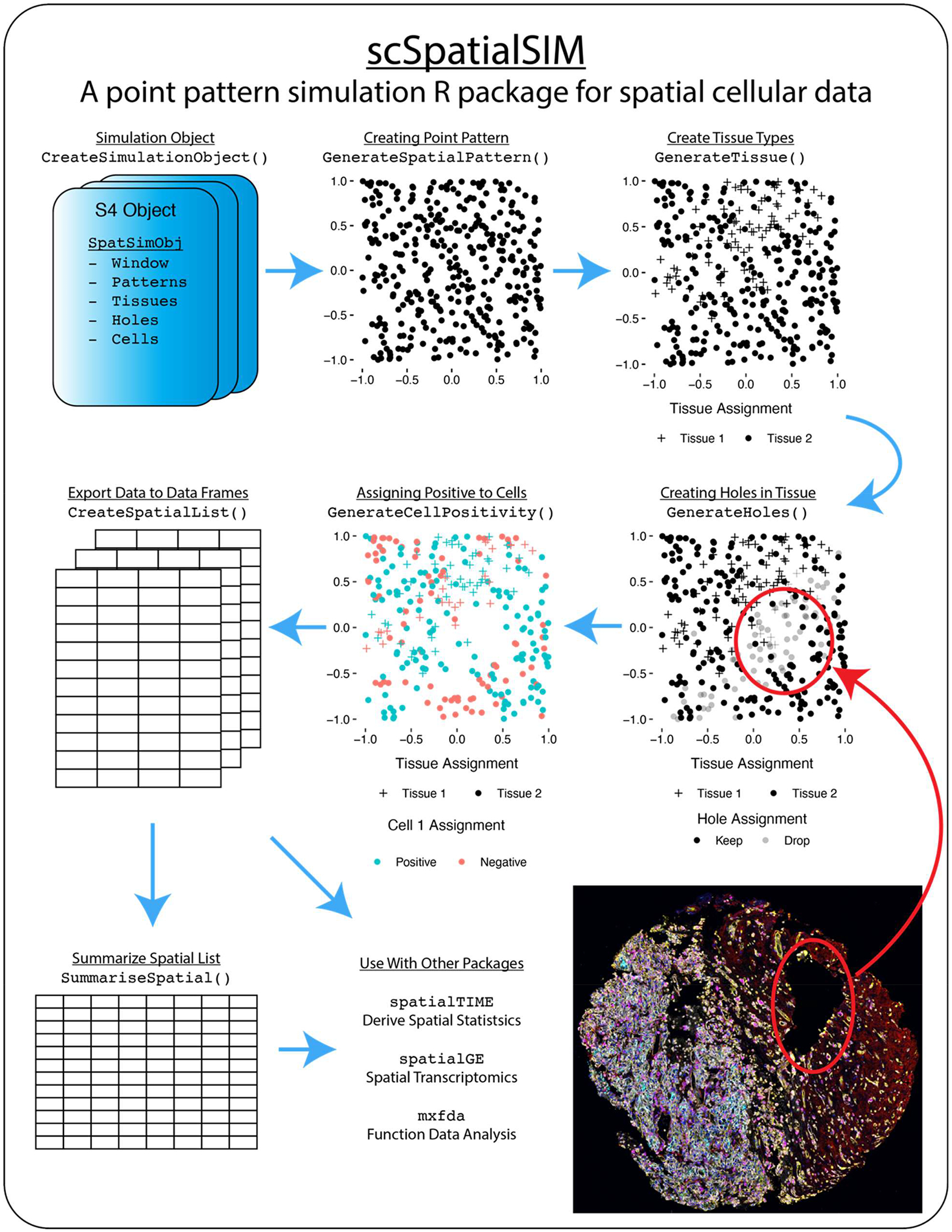 Figure 1
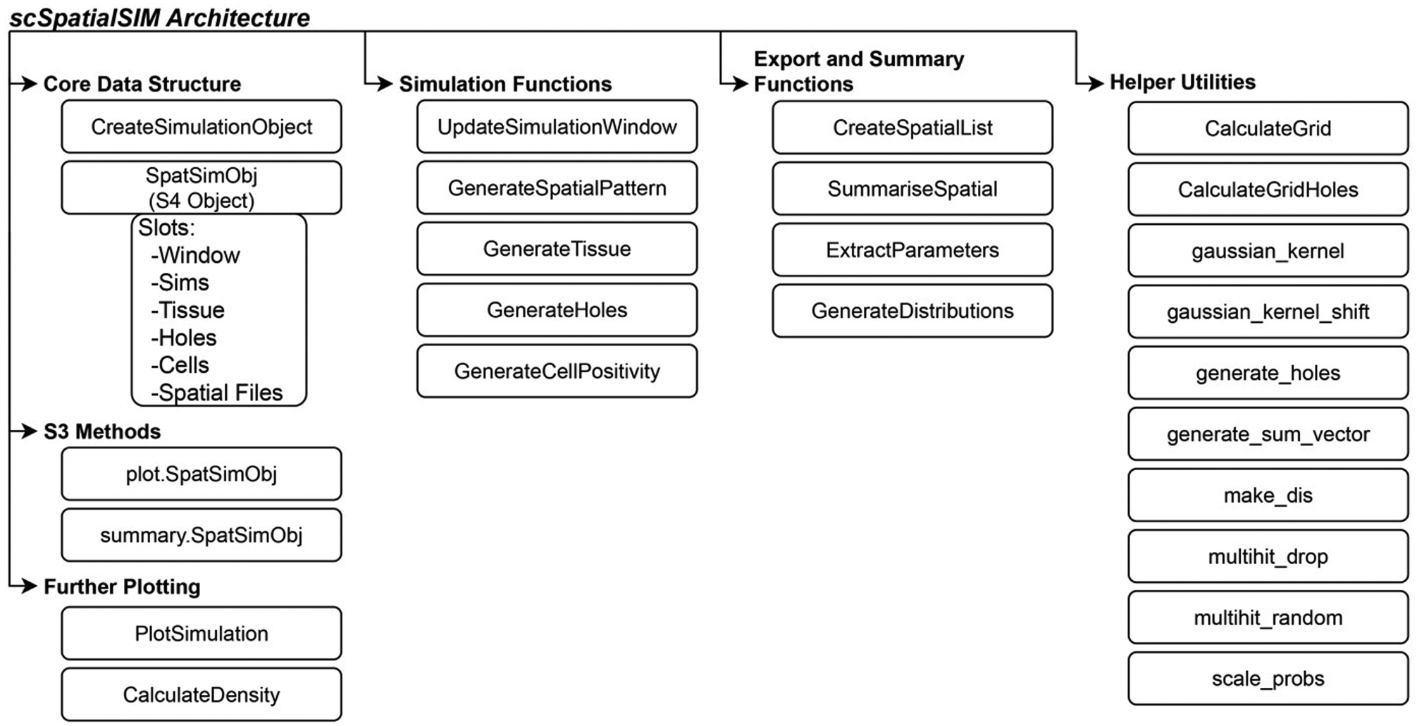 Figure 2
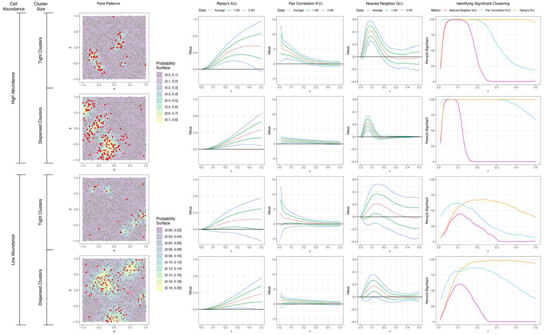 Figure 3
| Nr | Code metadata description | Metadata |
|---|---|---|
| C1 | Current code version |
|
| C2 | Permanent link to code/repository used for this code version | |
| C3 | Permanent link to reproducible capsule | |
| C4 | Legal code license |
|
| C5 | Code versioning system used |
|
| C6 | Software code languages, tools and services used | R |
| C7 | Compilation requirements, operating environments and dependencies | R (≥4.0) |
| C8 | If available, link to developer documentation/manual |
|
| C9 | Support email for questions |
|
Peer Reviews
No public reviews on file for this paper yet. If you reviewed it on a platform where reviews are public (OpenReview, ICLR, NeurIPS, ICML), you can paste yours below so the community can read it here.
Videos
No videos yet. Explain this paper in a talk, walkthrough, or lecture? Add one.
Taxonomy
TopicsSingle-cell and spatial transcriptomics · Cell Image Analysis Techniques · Advanced Fluorescence Microscopy Techniques
Metadata
**: **
Motivation and significance
Studying the spatial contexture of cells in biological tissues is increasing in popularity among biomedical researchers. New technologies allow the profiling and phenotyping of cells in tissue microarrays (TMAs) and whole tissue slides to understand the spatial architecture of tissues, such as the tumor microenvironment (TME), and the distributions of cells in 2-dimensional space. The ability to characterize the spatial context of cells has allowed for further exploration of the correlation between the tissue architecture and patient outcomes, such as overall survival or response to therapies [1–3]. In contrast to studying only the cell abundance or density, the spatial architecture of cell types and their level of aggregation or dispersion can provide more details about the organization of complex tissues and answer important questions about cell-cell communication and their associations [3,4].
Single-cell protein imaging platforms like multiplex immunofluorescence (mIF) or immunohistochemistry [5], have been successfully used to profile cell types in tissues, as well as spatially characterize the immune microenvironment of several malignancies [3,6]. In addition to single-cell protein data, spatially resolved transcriptomics (SRT) has recently gained traction in biological research. SRT experiments can range from studies involving imaging or sequencing regions of tissue (GeoMx [7], Nanostring, Seattle, WA) to equally spaced grids with unique molecular identifiers and spatial barcodes containing between 5 and 10 cells (Visium [8], 10x Genomics, Pleasanton, CA) to sub-cellular transcript locations (CosMx Spatial Molecular Imaging [9], Nanostring, Seattle, WA; Xenium [10], 10x Genomics). These spatial molecular technologies require complex statistical and bioinformatic approaches to summarize the spatial characteristics of the tissues. Statistical methods from the field of ecology have been used to assess the level of clustering of cell types in tissues, but there is a lack of consensus on which method is the “gold standard”. Along with lacking a ‘gold standard’, methods for analyzing the spatial contexture of cells in both spatial proteomics and SRT continue to be developed rapidly yet lack the ways for which to objectively evaluation them against existing methods.
To bridge this gap in the literature, we have developed an R package, “scSpatialSIM”, that allows for fine-tuned simulation of spatial single-cell molecular data which can be exported in formats that are common for the field (i.e., HALO from Indica Labs for digital pathology; “scSpatialSIM” workflow is displayed in Fig. 1). This package can be used to compare available statistical methods for measuring clustering and co-localization of single-cell spatial data as well as benchmark new methods as they are developed. While packages like “spaSim” [11], “scCube” [12], “scDesign3” [13], and “SRTsim” [14] exist to simulate cell-level data to mimic tissue architectures and domains, “scSpatialSIM” can simulate cell phenotypes (categorical) and continuous data (e.g., mIF intensity data, SRT gene expression data) depending on user input and parameter settings without requiring training data. Table 1 display comparisons between these simulation methods. The distributions of protein or gene expression for positive and negative cells can be finely adjusted to assess spatial clustering and co-localization method sensitivity.
Software description
“scSpatialSIM” is an R package designed to simulate spatial single-cell molecular data, offering researchers a flexible and efficient platform for creating biologically realistic spatial data to benchmark clustering methods. The package supports installation on R4.0.0 or later and is available from GitHub and CRAN. Many of the functions from “scSpatialSIM” support piping (i.e., using the magrittr %>% function) which allows function calls to be chained together to develop whole simulation pipelines from start to finish. Once scenarios have been simulated, “scSpatialSIM” can export the results as tabular data (i.e., Indica Labs’ HALO) for use in external tools to assess power of spatial clustering methods. Additionally, we have created vignettes (https://fridleylab.github.io/scSpatialSIM) that demonstrate how to use “scSpatialSIM” as well as how the outputs of “scSpatialSIM” can be input into other R packages to derive spatial statistics, such as with the R package “spatialTIME” [15].
Software architecture
2.1.
“scSpatialSIM” uses an S4 object (class SpatSimObj) which serves as storage for all the parameters and results performed with “scSpatialSIM”. Our goal was to provide a collection of methods that allow for the creation of realistic simulations of cell types within tissue samples in a stepwise manner: 1) point patterns, 2) tissue regions or domains, 3) holes/non-cellular areas, and 4) cell phenotypes. Fig. 2 shows the architecture of “scSpatialSIM”. The SpatSimObj also stores the simulation space (class òwin` from “spatstat” [16]), the number of independent simulations to perform, and the number of cell types to simulate.
Software functionalities
2.2.
The simulation functionality of “scSpatialSIM” is handled largely through 5 functions from the creation of the SpatSimObj object to generating cell positivity from the probability surfaces:
- CreateSimulationObject(): Creates the S4 object that maintains information about the simulation scenario from the simulation window (“spatstat” object class owin), the number of simulations, and the probability surface layers with their respective parameters. Additionally, the number of cell types wanting to be simulated is stored here (one cell type for benchmarking clustering, or more than one for benchmarking colocalization)
- GenerateSpatialPattern(): Generates spatial point patterns using “spatstat” rpoispp(). This point pattern represents the underlying point pattern of the whole sample.
- GenerateTissue(): Generates a probability surface based on input parameters for regions that will be “Tissue 1″, with areas of low probability being assigned “Tissue 2”.
- GenerateHoles(): Generates a probability surface based on input parameters for which points in the point pattern have a feature of ‘hole’ for evaluating spatial metrics ability to compensate for violations of stationarity.
- GenerateCellPositivity(): Generates probability surfaces based on input parameters and number of cell types set in the SpatSimObj. This results in cells being labelled as positive and negative. This function also allows for shifting of the probability surfaces between multiple cell types
Further, GenerateDistributions() can be used to generate distributions on positive and negative cells (i.e., protein abundance, gene expression, etc.) to assess power of spatial functions to pick up varying degrees in shifts spatially between cells types.
During the simulation process, there is the ability to calculate probabilities at differing spatial resolutions in functions used to calculate probability surfaces. If probabilities at the different resolutions are not initially calculated (desired if simulating many samples in a scenario), CalculateDensity() is able to calculate them at a later step for visualization. PlotSimulation() allows for plotting of these probabilities as a heatmap to visualize the probability surface used for cell assignments. It is also able to plot the whole core after cells have been assigned to the tissues, holes, and cell types. A basic point pattern is able to be visualized using the S3 plot method from ‘spatsat’ [16].
To provide the data in formats that are typical outputs from software suits like Indica Labs’ HALO and input formats for tools like “spatialTIME” or “spatstat”, we’ve included CreateSpatialList() that returns a list of data frames, one for each sample (each row a cell). Often these data frames are also summarized at the sample or image level, with each row containing number of cells and cell abundance for a sample, which can be calculated with SummariseSpatial().
Illustrative examples
To demonstrate the utility of “scSpatialSIM”, we will use the example of benchmarking the univariate spatial summary functions Ripley’s K, Nearest Neighbor G, and Pair Correlation g with 4 simulation scenarios that differ in abundance and size of clusters. Benchmarking of the spatial summary functions can have two separate components: 1) which spatial summary function is able to identify the most samples in a scenario with significant clustering, and 2) how many radii does each spatial summary function identify 100 % of samples with significant clustering. Significant clustering is assessed through a permutation approach to determine the empirical distribution of randomness.
scSpatialSIM example code
3.1.
#Create simulation object with 1000 samples in a 2×2 window, centered at 0 R> obj = CreateSimulationObject(sims = 1000,
- window = spatstat.geom::owin(c(−1, 1), c(−1, 1))) #generate spatial point pattern with a point (cell) intensity of 250 per unit area R> obj = GenerateSpatialPattern(obj,
- lambda = 250) #generate probability surface and assign points (cells) to holes, with default parameters R> obj = GenerateHoles(obj, density_heatmap = FALSE,
- cores = 5, use_window = TRUE) #generate probability surface and assign points (cells) to tissues, with default parameters R> obj = GenerateTissue(obj, density_heatmap = FALSE,
- cores = 5, use_window = TRUE) #generate positivity for cells – since univariate shift won’t be used #simulating 5 clusters (k = 5) #tight clusters (small sdmin and sdmax) #high abundance (probs between 0.01 and 0.75 for probability surface scaling) R> obj = GenerateCellPositivity(obj,
- k = 5, sdmin = 0.1, sdmax = 0.3,
- probs = c(0.01, 0.75), use_window = TRUE) #extract the new spatial samples and summarise at sample level R> spat_list = CreateSpatialList(obj) R> sum_data = SummariseSpatial(spatlist, ‘Cell 1 Assignment’)
Different simulation scenarios
3.2.
Running “scSpatialSIM” for 4 different scenarios provides different degrees of clustering to test the spatial summary functions under. Table 2 shows the different scenarios simulated with varying clusters size (Cluster Variation) and abundance (Cell Abundance). These parameters can be gathered from biological samples to replicate real-world tissues.
Assessing spatial summary functions
3.3.
Using these simulated scenarios, we applied spatial summary functions within the “spatialTIME” package R package (Ripley’s K, Nearest Neighbor G, and Pair Correlation g). A total of 100 permutations were used to estimate the deviation of real Cell 1 Assignment locations from the empirical distribution of randomness, and each function was estimated at radii from 0 to 0.5 at increments of 0.01. Fig. 3 shows example sample plots for the 4 scenarios as well as Degree of Clustering Permutation from “spatialTIME” averaged over all samples (with mean and standard deviations).
The results of the “scSpatialSIM” simulated data show that Ripley’s K identifies significant cell clustering across more radii than Nearest Neighbor G and Pair Correlation g (Table 3 – Most Significant). Scenarios with high abundance (Scenario 1 and 2) also showed more radii with all simulated samples with significant clustering for Ripley’s K and Pair Correlation g. Nearest Neighbor G did not identify more samples with significant clustering at any radii, and only identified all simulated samples having significant clustering at a single radius.
Impact
Spatial profiling is constantly increasing in usage in biological sciences [17], and with it new spatial methods are being developed in attempt to better capture tissue features. However, there is little means of comparing methods objectively and under which environments the methods are best suited. “scSpatialSIM” is an easy and fast software that allows for the fine-tuned simulation of biologically-informed clustering without the requirement for training data. With “scSpatialSIM”, researchers are now able to quickly benchmark spatial clustering methods at scale, including those meant for assessing spatial autocorrelation (demonstrated in vignette “Adding Continuous Cell Attributes”) and even impacts that violations of stationarity may result in (like necrotic tissue or tissue folds during sectioning). Previously, we have showed it’s utility in benchmarking bivariate spatial summary functions assessing immune cell colocalization in ovarian and lung cancer tumors [18]. Though, while the software focuses on single-cell molecular data it can directly be used as demonstrated here in other fields such as ecology.
“scSpatialSIM” is meant to simulate single cell clustering, or two or more cell colocalization. While it does lack the ability to simulate more complex tissue domains or regions that may be important for benchmarking methods designed to identify them, “scSpatialSIM” excels at its primary goal: providing a robust and scalable platform for benchmarking spatial statistics. With this software, researchers will be better able to benchmark new spatial clustering methods and select those that best answer their research questions.
Conclusions
“scSpatialSIM” is an important software for advancing spatial biology and method development. With its ability to simulate different clustering scenarios at scale, it will help identify correct methods to accurately answer biological questions. Further, since “scSpatialSIM” exports data in formats that are easily used in other packages that assess spatial clustering, it streamlines the process of benchmarking.
The reference list from the paper itself. Each links out to its DOI / PubMed record.
- 1Steinhart B, The spatial context of tumor-infiltrating immune cells associates with improved ovarian cancer survival. Mol Cancer Res 2021;19(12):1973–9.34615692 10.1158/1541-7786.MCR-21-0411 PMC 8642308 · doi ↗ · pubmed ↗
- 2Tan WCC, Overview of multiplex immunohistochemistry/immunofluorescence techniques in the era of cancer immunotherapy. Cancer Commun 2020;40(4):135–53 (Lond).
- 3Wilson C, Tumor immune cell clustering and its association with survival in African American women with ovarian cancer. P Lo S Comput. Biol 2022;18(3): e 1009900.35235563 10.1371/journal.pcbi.1009900 PMC 8920290 · doi ↗ · pubmed ↗
- 4Soupir AC, Increased spatial coupling of integrin and collagen IV in the immunoresistant clear-cell renal-cell carcinoma tumor microenvironment. Genome Biol. 2024;25(1):308.39639369 10.1186/s 13059-024-03435-z PMC 11622564 · doi ↗ · pubmed ↗
- 5Barua S, A functional spatial analysis platform for discovery of immunological interactions predictive of low-grade to high-grade transition of pancreatic intraductal papillary mucinous neoplasms. Cancer Inform 2018;17: 1176935118782880.
- 6Peng H, Multiplex immunofluorescence and single-cell transcriptomic profiling reveal the spatial cell interaction networks in the non-small cell lung cancer microenvironment. Clin Transl Med 2023;13(1):e 1155.36588094 10.1002/ctm 2.1155 PMC 9806015 · doi ↗ · pubmed ↗
- 7Zollinger DR, Geo Mx™ RNA assay: high multiplex, digital, spatial analysis of RNA in FFPE tissue. Methods Mol Biol 2020;2148:331–45.32394392 10.1007/978-1-0716-0623-0_21 · doi ↗ · pubmed ↗
- 8Applicaiton Note - enriching pathological analysis of FFPE tumor samples with spatial transcriptomics. Document number LIT 000152, 10x genomics, 2021.