Simulation of citrus foliar gas exchange across diverse meteorological conditions: application of the optimal stomatal regulation method
Mengying Fan, Zhihui Wang, Xuelian Jiang, Ningbo Cui, Jingtian Zhao, Shouzheng Jiang, Guoyu Zhu, Liwen Xing, Xiaoxian Zhang

TL;DR
This paper uses optimal stomatal regulation theory to simulate gas exchange in citrus leaves under various weather conditions, offering a practical model for orchard management.
Contribution
The study introduces and evaluates a family of optimal stomatal conductance-based models for simulating citrus leaf gas exchange.
Findings
The OSCvjd model showed the highest accuracy in predicting stomatal conductance with an R2 of 0.73.
The OSC model best simulated intercellular CO2 concentration and photosynthesis with R2 values of 0.78 and 0.48, respectively.
Model performance was best under moderate meteorological conditions with a 35.2% mean absolute relative error for stomatal conductance.
Abstract
The optimal stomatal regulation theory provides an eco-evolutionary framework for interpreting the trade-off between CO2 uptake and water loss. This theory postulates that the marginal water cost of carbon gain (λ=∂E/∂A) remains approximately constant over short timescales, thereby offering a mechanistic basis for predicting stomatal behavior and gas exchange. In this study, leaf-level meteorological variables and gas exchange parameters of orchard citrus were measured throughout the entire phenological period during 2021–2022. We developed a family of optimal stomatal conductance-based models (OSCMs), comprising six forms: Rubisco-limited forms (OSCvc and OSCvcd), RuBP-regeneration-limited forms (OSCvj and OSCvjd), and combined forms that dynamically select the prevailing biochemical limitation (OSC and OSCd). The key parameter λ was estimated daily and averaged over the entire…
Genes, proteins, chemicals, diseases, species, mutations and cell lines named across the full text — each resolved to its canonical identifier and authoritative record.
Click any figure to enlarge with its caption.
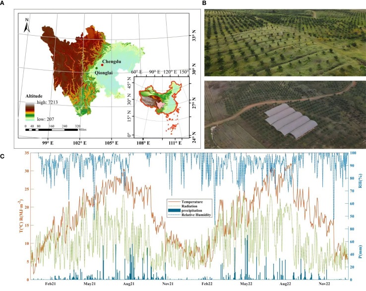 Figure 1
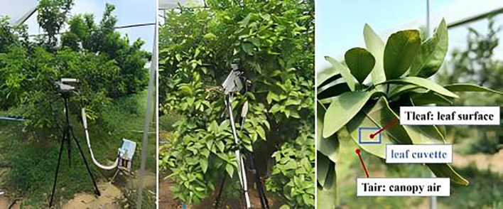 Figure 2
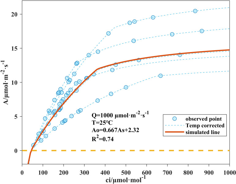 Figure 3
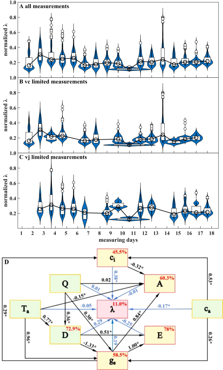 Figure 4
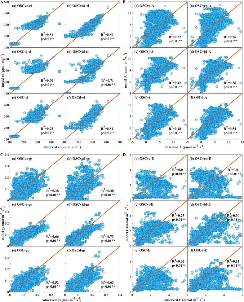 Figure 5
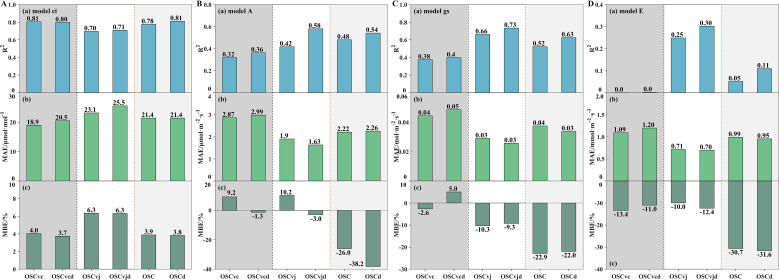 Figure 6
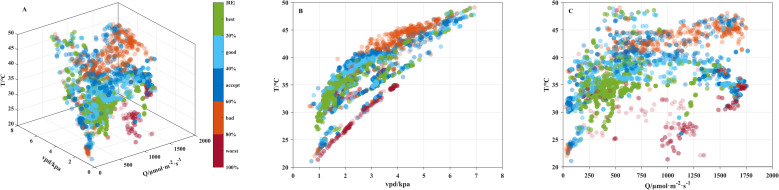 Figure 7
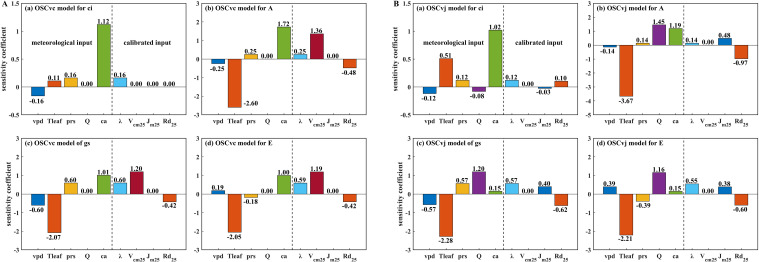 Figure 8
| Order | Date (yyyy-mm-dd) | Time | Measure | Weather | Average soil moisture (%) |
|---|---|---|---|---|---|
| 1 | 2021-04-29 | 9:00-17:00 | 325 | sunny | 26.49 |
| 2 | 2021-06-29 | 9:30-12:00 | 80 | overcast | 26.60 |
| 3 | 2021-07-02 | 10:00-18:00 | 141 | cloudy | 24.45 |
| 4 | 2021-07-03 | 10:00-18:00 | 115 | overcast | 22.66 |
| 5 | 2021-07-20 | 10:00-17:00 | 67 | overcast | 21.66 |
| 6 | 2021-07-31 | 9:00-17:30 | 113 | sunny | 26.75 |
| 7 | 2021-08-02 | 9:30-10:30 | 37 | cloudy | 26.06 |
| 8 | 2021-08-06 | 9:30-10:30 | 37 | sunny | 24.09 |
| 9 | 2021-09-15 | 9:00-12:00 | 86 | cloudy | 24.43 |
| 10 | 2022-04-29 | 9:00-12:00 | 26 | cloudy | 23.62 |
| 11 | 2022-06-24 | 9:00-12:00 | 28 | cloudy | 26.70 |
| 12 | 2022-07-06 | 9:00-16:00 | 302 | overcast | – |
| 13 | 2022-07-07 | 9:00-12:00 | 226 | overcast | – |
| 14 | 2022-07-21 | 9:00-12:00 | 86 | overcast | 26.80 |
| 15 | 2022-07-22 | 10:00-13:00 | 76 | overcast | 26.80 |
| 16 | 2022-08-09 | 9:00-11:30 | 26 | cloudy | 22.58 |
| 17 | 2022-10-01 | 10:00-10:30 | 81 | cloudy | 26.83 |
| sum | 1852 | ||||
| Symbol | Descriptions | Units | Source | Value |
|---|---|---|---|---|
|
| net photosynthetic rate | μmol·m-2·s-1 | meas | |
|
| transpiration rate | mmol·m-2·s-1 | meas | |
|
| stomatal conductance to water | mol·m-2·s-1 | meas | |
|
| intercellular CO2 concentration | μmol·mol-1 | meas | |
|
| photosynthetic photon flux density | μmol·m-2·s-1 | meas | |
|
| Leaf surface air temperature | °C | meas | |
|
| leaf temperature | °C |
| |
|
| leaf kelvin temperature | K | ||
|
| vapor pressure deficit | kPa | meas | |
|
| ambient CO2 concentration | μmol·mol-1 | meas | |
|
| air pressure of the atmosphere on leaf surface | kPa | meas | |
|
| limited carboxylation rate by Rubisco | μmol·m-2·s-1 | Eq. 2 | |
|
| limited carboxylation rate by RuBP | μmol·m-2·s-1 | Eq. 3 | |
|
| CO2 compensation concentration at chloroplast thylakoids | μmol·mol-1 | Eq. 5 | |
|
| mitochondrial respiration rate under light | μmol·m-2·s-1 | Eq. 4 | |
|
| mitochondrial respiration rate under light at 25°C | μmol·m-2·s-1 | cali | 1.77 |
|
| maximum rate of Rubisco carboxylation activity | μmol·m-2·s-1 | Eq. 4 | |
|
| maximum rate of Rubisco carboxylation activity at 25°C | μmol·m-2·s-1 | cali | 43.21 |
|
| Michaelis Menten coefficients of Rubisco activity | μmol·mol-1 | Eq. 2 | |
|
| Michaelis Menten coefficients of Rubisco activity for CO2 | μmol·mol-1 | Eq. 6 | |
|
| Michaelis Menten coefficients of Rubisco activity for O2 | mmol·mol-1 | Eq. 7 | |
|
| intercellular O2 concentration | mmol·mol-1 | coef | 210 |
|
| potential maximum rate of electron transport | μmol·m-2·s-1 | Eq. 4 | |
|
| potential maximum rate of electron transport at 25°C | μmol·m-2·s-1 | cali | 75.56 |
|
| electron transport rate | μmol·m-2·s-1 | Eq. 3 | |
|
| quantum yield of electron transport | coef | 0.24 | |
|
| gas constant | J·mol-1·K-1 | coef | 8.314 |
|
| entropy term | J·mol-1·K-1 | coef | 629.26 for |
|
| rate of exponential increase of the biochemical parameters below the optimum temperature | J·mol-1 | coef | 58550 for |
|
| rate of decrease of the biochemical parameters above the optimum temperature | J·mol-1 | coef | 200,000 |
|
| mesophyll conductance | mol·m-2·s-1 | infinity | |
|
| CO2 concentration in the carboxylation site of chloroplast thylakoids | μmol·mol-1 |
| |
|
| simulated net photosynthetic rate under Rubisco limitation | μmol·m-2·s-1 | Eq. 9 | |
|
| simulated net photosynthetic rate under RuBP limitation | μmol·m-2·s-1 | Eq. 9 | |
|
| marginal water cost for unit carbon assimilation | mol·mol-1 | Eq. 13 |
| Order | Date (yyyy-mm-dd) | Median value of | Median value of | Median value of |
|---|---|---|---|---|
| 1 | 2021-04-29 | 520.89 | 525.86 | – |
| 2 | 2021-06-29 | 1,643.41 | 1,667.70 | 1,321.57 |
| 3 | 2021-07-02 | 2,138.93 | 1,780.99 | 3,248.67 |
| 4 | 2021-07-03 | 2,570.25 | 2,240.79 | 2,802.25 |
| 5 | 2021-07-20 | 2,922.37 | – | 2,922.37 |
| 6 | 2021-07-31 | 1,215.57 | 1,191.83 | 1,954.64 |
| 7 | 2021-08-02 | 1,458.09 | 1,458.09 | – |
| 8 | 2021-08-06 | 1,810.29 | – | 1,840.31 |
| 9 | 2021-09-15 | 1,625.71 | 1,599.26 | 3,208.17 |
| 10 | 2022-04-29 | 426.87 | 360.87 | 594.94 |
| 11 | 2022-06-24 | 2,029.29 | 1,511.00 | 2,888.72 |
| 12 | 2022-07-06 | 2,000.97 | 1,696.35 | 3,033.92 |
| 13 | 2022-07-07 | 3,135.39 | 3,134.98 | – |
| 14 | 2022-07-21 | 1,769.87 | 1,228.22 | 2,072.09 |
| 15 | 2022-07-22 | 2,443.56 | 2,032.39 | 2,958.37 |
| 16 | 2022-08-09 | 2,448.98 | 2,378.56 | 2,548.55 |
| 17 | 2022-10-01 | 2,689.75 | – | 2,691.51 |
| median | 1,787.10 | 1,478.51 | 2,703.65 | |
| Order | Tl | Km | Γ* | Vcmax25 | Jmax25 | Rd25 |
|---|---|---|---|---|---|---|
| units | °C | μmol ·m-2·s-1 | μmol ·mol-1 | μmol ·m-2·s-1 | μmol ·m-2·s-1 | μmol ·m-2·s-1 |
| 1 | 31.06 | 1,173.59 | 54.60 | 39.09 | 68.87 | 1.45 |
| 2 | 33.13 | 1,406.20 | 60.43 | 56.58 | 86.11 | 2.58 |
| 3 | 29.18 | 1,000.11 | 50.21 | 24.53 | 54.20 | 1.72 |
| 4 | 36.69 | 1,911.34 | 71.66 | 43.98 | 65.02 | 2.30 |
| 5 | 27.81 | 885.32 | 46.47 | 51.85 | 103.61 | 0.81 |
| average | 43.21 | 75.56 | 1.77 |
Peer Reviews
No public reviews on file for this paper yet. If you reviewed it on a platform where reviews are public (OpenReview, ICLR, NeurIPS, ICML), you can paste yours below so the community can read it here.
Videos
No videos yet. Explain this paper in a talk, walkthrough, or lecture? Add one.
Taxonomy
TopicsPlant Water Relations and Carbon Dynamics · Greenhouse Technology and Climate Control · Plant Physiology and Cultivation Studies
Introduction
1
Citrus, characterized by millennia-long cultivation history, extensive varietal diversity, distinctive flavors, and high nutritional value, plays an essential role in human diet and agro-processing industry (Palangasinghe et al., 2024). As for 2023, the global citrus planting area has exceeded 8.76×10^6^ hectares and the annual production has reached 1.35×10^8^ tons (FAOSTAT, 2025). China contributes nearly 30% of global citrus production, making citrus cultivation a critical component of its agricultural economy, particularly in the hilly regions of Southwest China (Wang et al., 2022). However, regional water scarcity and frequent seasonal droughts have impeded sustainable citrus production (Dong et al., 2024). Such water-related constraints highlight the importance of stomatal regulation in coordinating water loss and carbon assimilation.
Stomata, the primary low-resistance gateway for leaf-atmosphere gas exchange, affect photosynthesis and transpiration directly (Negi et al., 2014). Stomatal function is especially dominant in citrus, where thick cuticles substantially restrict gas diffusion through epidermis (Tominaga and Kawamitsu, 2024). Stomatal aperture can rapidly respond to biotic and abiotic changes, while stomatal anatomy and density adapt more slowly to local climates over evolutionary time (Hetherington and Woodward, 2003). Field studies illustrate pronounced spatiotemporal variability in citrus stomatal behavior: well-managed Citrus sinensis L. in South Africa showed seasonal variation with peak stomatal conductance (g_s_) of 0.14 mol·m^-2^·s^-1^ in warm Autumn (Munjonji et al., 2021). In southeastern Brazil, an increase in atmospheric vapor pressure deficit (D) from 1.0 to 3.0 kPa reduced g_s_ by 51% (Souza et al., 2004). On Corsica Island in southern France, the g_s_ of Citrus deliciosa Ten. and Citrus maxima Merr. declined by 33–34% during the cold period, whereas the reduction reached 67% in Citrus medica L (Santini et al., 2012). Although many studies have investigated citrus stomatal responses, observed patterns differ across regions, climates, and cultivars, highlighting the complexity of stomatal regulation. Therefore, a unified theoretical framework is needed to interpret and predict stomatal behavior across diverse environments.
Researchers have proposed multiple explanations for stomatal behavior. Some argue that stomata respond directly to environmental factors (Jarvis and P., 1976), whereas others suggested that stomatal movement covaries with photosynthesis under given conditions (Ball et al., 1987), and still others emphasized the regulatory role of internal leaf states such as water potential, ion fluxes and cell turgor (Buckley et al., 2003; Delwiche and Cooke, 1977). Amid these diverse perspective, Cowan and Farquhar (1977) proposed a theory of optimal stomatal regulation from an evolutionary and philosophical interpretative angle: an acclimated plant would maximize its carbon gain over a finite water supply, mathematically formulated as maximizing the time integral of A-E/λ. Here, parameter λ—the marginal water cost of carbon gain (∂E/∂A)—is typically assumed to be constant over short timescales and adjusted to soil water availability over long timescales (Manzoni et al., 2013). Experimental evidence supporting this framework has been reported for numerous species (Buckley, 2005). However, findings in more complex environments are mixed, prompting further debates on its foundations and applicability. Katul et al. (2010) observed the individual leaf λ of Pinus taeda L. of North Carolina was steady on short-term but decreased with elevated atmospheric CO_2_ resulting from prescribed burning. The fluctuations in λ with temperature were also observed on Oryza sativa L. and Triticum aestivum L (Huang et al., 2021). Severe water or heat stress disrupt leaf internal hydraulic and biochemical status, imposing hydraulic failure or non-stomatal limits that violate the optimality assumption (Marchin et al., 2023; Potkay et al., 2025b).
Although uncertainties regarding λ variability and model implementation persist, the optimality theory continues to be widely adopted in both empirical and modeling studies (Wang et al., 2020). Finally, two approaches have emerged for applying the optimality theory (Knauer et al., 2018; Manzoni et al., 2011): 1) deriving λ analytically from plant gaseous exchange measurements and using its variation to diagnose plant stress; 2) predicting plant gaseous exchange using a prescribed λ. These two applications constitute the focus of our study, which applies the optimality theory to a citrus orchard in southwestern China and evaluates its applicability.
Directly solving the Lagrange multiplier under optimal hypothesis (λ=∂E/∂A) is inherently challenging (Buckley and Mott, 2013). Some researchers estimate instantaneous λ by combining foliar environment variables with gas exchange measurements through physically based or empirical formulations (Medlyn et al., 2013; Volpe et al., 2011). The accuracy of λ derived by these approaches depends critically on the quality of input data and the suitability of the computational method employed (Thomas et al., 1999). Beyond gas exchange-based methods, characteristic λ values can also be inferred from correlated factors such as vegetation type, soil moisture, plant water potential, and atmospheric CO_2_ concentration (Lin et al., 2015; Liu et al., 2022; Wang et al., 2019).
From a theoretical perspective, optimal stomatal conductance models provide a mechanistic framework linking carbon assimilation and water loss through the Lagrange multiplier λ, offering a physiologically interpretable basis for predicting gas exchange. By reversing the causal direction in the calculation and prescribing an empirically known λ first, gas exchange can be predicted from environmental factors (Mrad et al., 2019). Transforming λ into g_s_ requires gas exchange equations, typically Fick’s law of gas diffusion and the Farquhar biochemical model due to their mechanistic basis and minimal empiricism (Medlyn et al., 2011). These coupled optimal stomatal conductance-based models (OSCMs) can simultaneously solve for stomatal conductance (g_s_), photosynthesis (A), transpiration (E) and intercellular CO_2_ concentration (c_i_) using species traits and atmospheric inputs without cumbersome calibration work. Within this framework, plant gas exchange variables are often predicted with high fidelity (Buckley and Mott, 2013). Ji et al. (2017) predicted the g_s_ of well-watered soybean and maize with R^2^ value of 0.86 and 0.88, respectively. Lu et al. (2016) successfully captured the responses of A, E and water use efficiency (WUE) along rainfall gradients across diverse forest sites.
In addition, two uncertainties arise in the application of the OSCMs. First, as research on stomatal behavior advances, evidence suggest that using hydraulic structural risks rather than transpiration water loss may more accurately represent the water cost for plants (Dewar et al., 2018; Wolf et al., 2016). Accordingly, the assumption of a constant Lagrange multiplier λ should be applied with caution, especially in arid regions (Potkay et al., 2025a; Venturas et al., 2018). Second, within the sub-equation of the OSCMs, the Farquhar functions adopt two different forms depending on photosynthetic limitations: either the CO_2_ carboxylation rate (Rubisco) or the electron transport rate (RuBP) (Vico et al., 2013). Some studies have preferred to assume a single dominant limitation to achieve a neat analytical expression and smooth solutions (Katul et al., 2010; Schymanski et al., 2015). However, in natural environments, limitations may shift due to fluctuations in water availability, light, temperature, and various other abiotic factors (Abdulbaki et al., 2022; Perdomo et al., 2017).
In this study, two years of citrus leaf gas exchange data were collected from a citrus orchard in southwestern China. Analytical λ under diverse meteorological conditions were examined and the applicability of the conventional optimal stomatal model was discussed. Our objectives were to: 1) calculate the marginal water cost of carbon gain λ and determine its characteristic values for citrus; 2) modify the optimal stomatal conductance-based models (OSCMs) by distinguishing Rubisco and RuBP scenarios, acknowledging that photosynthetic limitations may vary under different environmental conditions, and predict citrus gas exchange; 3) analyze the main factors affecting model performance and recommend suitable environmental conditions for its application. This research aims to enhance understanding of citrus foliar gas exchange and stomatal regulation in seasonal arid regions and provide a low-input method for forecasting agricultural water-carbon fluxes.
Materials and methods
2
Experimental site
2.1
The measurements were conducted on six-year-old citrus (Citrus Tachibana Tanaka.) grafted onto tangerine rootstock (Citrus Reticulata Blanco.) during the phenological period (March–November) in an artificial citrus orchard in Qionglai city, Sichuan province, China (103.45°E, 30.34°N). The citrus orchard is situated at an altitude of 547 m in a subtropical monsoon climate zone characterized by abundant but seasonally uneven rainfall and solar radiation. The multi-year averages of air temperature, relative humidity, and annual precipitation were 16.8 °C, 82%, and 1041.3 mm, respectively. During the two experimental years, the mean air temperature, humidity, solar radiation, and annual precipitation were 17.6 °C, 93.2%, 10.2 MJ·m^-2^·day^-1^, and 1013.7 mm, respectively (Figure 1).
Geographic location and climatic condition of experimental site.
The experimental aerated greenhouse was located in a shallow hilly zone, with an average soil bulk density of 1.13 g·cm^-^³ and a maximum water-holding capacity (θ_f_) of 35.4% volume moisture content. Soil moisture was maintained at 60–75% θ_f_ through irrigation, with total irrigation amounts of 347.56 and 313.48 mm in 2021 and 2022, respectively. Fertilization during the entire phenological period totaled 1167 kg·hm^-2^, with a nutrient composition of 19-19-19 (N-P_2_O_5_-K_2_O) percent by weight. According to conventional management, the proportions of basal fertilizer and topdressing applied during the shooting, fruit setting, and fruit expanding stages were 2:1:3:4. Citrus trees were planted at a spacing of 4 m × 3 m. Vigorous citrus trees of similar growth, with height of 2.3–2.5 m, were selected for observation.
Measurement
2.2
Measurements of leaf gas exchange
2.2.1
Fully expanded citrus leaves on secondary shoots of similar sizes were selected for photosynthetic gas exchange measurements. For each tree, 4–6 leaves from two opposite orientations were tested without strictly distinguishing between sunlit and shaded positions (Figure 2). Gas exchange measurements were conducted as instantaneous observations on multiple leaves sampled at different times of the day; on full-day measurements, leaves measured in the morning were re-measured in the afternoon. Measurements were performed on rain-free days from April to October using infrared gas analysis systems (LI-6400XT, LI-COR Inc., Arizona, USA; Lcpro-SD, ADC Ltd., Hertfordshire, UK). At the start of each measurement day, the instrument was preheated for 30 minutes to routine check, including verifying the seal integrity of the leaf chamber and gas path, ensuring chemical effectiveness, and eliminating analyzer zero offset to guarantee data reliability. After validation, the selected functional leaves were tested in situ under ambient light conditions. A total of 1001 and 851 leaf gas exchange datasets were collected in 2021 and 2022, respectively (Table 1).
Leaf gas exchange measurements using a portable photosynthesis system.
Measurements of leaf net photosynthesis-CO2 response (A-ci) curve
2.2.2
On 22^nd^ April and 20^th^ October 2022, the response of functional leaves to varying CO_2_ concentrations were measured using a LI-6400XT system equipped with RGB red-blue light sources and a CO_2_ injection device. Prior to measurements, an eight-point calibration was performed to minimize the influence of ambient air fluctuations. Leaves were first acclimated for 30 min at a photosynthetically active radiation of 1000 μmol·m^-2^·s^-1^ and a CO_2_ concentration of 400 μmol·mol^-1^ until gas exchange parameters stabilized. Subsequently, CO_2_ concentrations in the cuvette were adjusted stepwise, and measurements at each level were recorded after stabilization or after a maximum of 5 min. The CO_2_ sequence was set as follows: 400, 300, 200, 150, 100, 50, 400, 400, 600, 800, 1000, 1200, 1500, 1800, and 2000 μmol·CO_2_·mol^-1^. During the curve measurements, temperature and humidity were not actively controlled to conserve battery power. However, both variables remained relatively stable throughout each test, and the resulting uncertainties were considered acceptable.
Parameter acquisition and model development
2.3
Calculation of photosynthetic characteristic parameters
2.3.1
The parameters including K_m_, Γ^^*, V_cmax25_, J_max25_, and R_d25_ were fitted from A-c_i_ curves based on the photosynthetic biochemical FvCB model and were assumed to be either constant or temperature-dependent, representing the photosynthetic traits of the studied citrus species. Under natural conditions, photosynthetic TPU limitation is rarely reached, rapidly transitioning to Rubisco-limited or RuBP-regeneration-limited states (Duursma, 2015; Rogers et al., 2021). Therefore, only the Rubisco and RuBP limitations were considered in this study. The FvCB model are shown in Equations 1–3 (Farquhar et al., 1980; Sharkey, 1985):
Where A is the net photosynthetic rate, μmol·m^-2^·s^-1^; w_c_ and w_J_ are the limited carboxylation rate by Rubisco and RuBP, respectively, μmol·m^-2^·s^-1^; Γ^^* is the CO_2_ compensation concentration at chloroplast thylakoids, μmol·mol^-1^; R_d_ is the rate of mitochondrial respiration under light, μmol·m^-2^·s^-1^; V_cmax_ is the maximum rate of Rubisco carboxylation activity, μmol·m^-2^·s^-1^; K_c_ and K_o_ are the Michaelis Menten coefficients of Rubisco activity for CO_2_ and O_2_, respectively; O is the intercellular O_2_ concentration, mmol·mol^−1^; J is the rate of electron transport, μmol·m^-2^·s^-1^; J_max_ is the potential maximum rate of electron transport, μmol·m^-2^·s^-1^; Q is the photosynthetic photon flux density, μmol·m^-2^·s^-1^; α is the quantum yield of electron transport, dimensionless; c_c_ is the CO_2_ concentration in the carboxylation site of chloroplast thylakoids, μmol·mol^-1^.
Parameters V_cmax_ and J_max_ are temperature-dependent and can be estimated from A-c_i_ curves, then normalized to 25°C using Equation 4 (Medlyn et al., 2002):
Where T_k_ is leaf kelvin temperature, K; R is the gas constant, J·mol^-1^·K^-1^; k_25_ is the biochemical parameters including V_cmax25_ and J_max25_, μmol·m^-2^·s^-1^; ΔS is entropy term, J·mol^-1^·K^-1^; E_a_ is the rate of exponential increase of the biochemical parameters below the optimum temperature, J·mol^-1^; H_d_ is the rate of decrease of the biochemical parameters above the optimum temperature, J·mol^-1^. The detailed values of ΔS, E_a_, and H_d_ for V_cmax25_ and J_max25_ are shown in Table 2.
Parameters Γ^^*, K_c_, and K_o_ also depend on temperature, calculated by Equations 5–7:
Assuming the mesophyll conductance (g_m_) approaches infinity, the CO_2_ concentration at the carboxylation site (c_c_) can be approximated by the intercellular CO_2_ concentration (c_i_) (Equation 8):
By substituting Equations 2, 3 into Equation 1, the simulated net photosynthetic rates under Rubisco limitation (A_c_) and RuBP limitation (A_j_) can be calculated, and the lower one was taken as the net photosynthesis rate. The photosynthetic characteristic parameters K_m_, Γ^^*, V_cmax25_, J_max25_, and R_d25_ were fitted from A-c_i_ response curve data using Equation 9, and the calibrated results are shown in Figure 3.
Fitted A-ci response curves. Points on the dashed lines are single-leaf measurements and corrected to 25 °C5 Solid lines are model simulations based on the average coefficients calibrated from the five measurement curves. Ao denotes the temperature-corrected observation leaf photosynthesis rate; As denotes the modeled rate calculated from the averaged coefficients at corresponding intercellular CO2 concentrations.
Calculation of the marginal water cost of carbon gain
2.3.2
The initial expression for the marginal water cost per unit carbon assimilation (λ) is given by Equation 10:
Where A is the net carbon assimilation rate, μmol·m^-2^·s^-1^; E is the water transpiration rate, mmol·m^-2^·s^-1^; g_s_ is the stomatal conductance, mol·m^-2^·s^-1^; a factor of 10^3^ is applied for unit consistency.
Assuming that mesophyll and boundary conductances are large enough to have a negligible impact, λ can be calculated using Equation 11 (Buckley et al., 2017):
Based on the FvCB functions (Equation 9), ∂A/∂c_i_ can be obtained as the partial derivative of A with respect to c_i_. Consequently, λ can be calculated by Equations 12, 13:
Establishment of the gs-E-A coupled optimal stomatal conductance-based models
2.3.3
The coupled optimal stomatal conductance-based models (OSCMs) are constructed by integrating three components: Fick’s gas diffusion law (Equation 14), the FvCB biochemical model (Equation 9), and the constant-λ optimal stomatal regulation hypothesis (Equation 15). The OSCMs can solve A, c_i_, E, and g_s_ simultaneously. The original equations are as follows:
Where P is the atmospheric pressure at the leaf surface, kPa.
The final formulas derived for Rubisco limitation (OSCvc model) are given in Equation 16:
The final formulas derived for RuBP limitation (OSCvj model) are given in Equation 17:
The coupled optimal stomatal conductance-based models (OSCMs) are established as Equations 16, 17, corresponding to the OSCvc and OSCvj forms. In these models, once c_i_ is determined from the topmost expression, it can be used in the subsequent equations to solve for A, g_s_, and E. To prevent negative simulated values of g_s_, a minimum stomata conductance (g_min_) of 0.01 mol·m^-2^·s^-1^ is imposed in this study.
The specific implementation steps of OSCMs are as follows: 1) Determining the photosynthesis characteristics parameters V_cmax25_, J_max25_, and R_d25_ from A-c_i_ curves and applying temperature correction; 2) Calculating the marginal water cost of carbon gain λ and determining a representative constant value; 3) Using OSCvc or OSCvj model to solve foliar gas exchange parameters including c_i_, A, E, and g_s_.
In steps 1–2, the characteristic coefficients are derived from surveyed gas exchange data, and can also be obtained from published studies on related species. In step 3, only c_a_, P, and D, are direct inputs for the OSCvc model (with Q added for the OSCvj model), while T_l_ or T_a_ is also necessary to adjust K_m_, Γ^^*, V_cmax_, J_max_, and R_d_ to actual temperature. Finally, based on the OSCMs, foliar gas exchange (A, E, c_i_, g_s_) can be simulated using species-specific parameters (V_cmax25_, J_max25_, R_d25_, λ) and meteorological inputs (c_a_, P, D, Q, T_a_).
Analysis
2.4
Analysis of parameter correlations
2.4.1
A structural equation model (SEM) incorporating meteorological parameters (c_a_, D, Q, T_a_), leaf gas exchange parameters (A, E, c_i_, g_s_), and the marginal water cost of carbon gain (λ) was established using SPSS Amos 28 (IBM Inc., Armonk, USA) to analyze the relationships between meteorological parameters and foliar gas exchange.
Model evaluation
2.4.2
The performance of the OSCMs models is evaluated by four indicators (Equations 18–21). The determination coefficient (R^2^) indicates the goodness of model fit, while the mean absolute error (MAE), relative mean bias error (MBE) and absolute relative error (RE) reflect model accuracy in terms of magnitude and proportion.
Where P_i_ is the predicted value of gas exchange indicators, and O_i_ is the corresponding observed value; and are the mean values of predicted and observed datasets, respectively. Model performance improves as MAE, MBE, and RE decrease and R^2^ approaches 1.
Model sensitivity
2.4.3
The model sensitivity coefficient quantifies the response of the model to variations in each input variable or parameter. A reference state was defined as an observed gas exchange data point under moderate meteorological conditions (T_a_ = 35°C, D = 2.0 kPa). The sensitivity coefficient (SC) was then calculated from OSC model simulations with perturbed inputs using Equations 22, 23:
Where S is the observed gas exchange value at the reference state, including g_s_, c_i_, A, and E; S_i_ is the corresponding simulated value with adjusted inputs; F is the observed value of a model factor at the reference state, including P, D, c_a_, Q, T_a_, λ, V_cmax25_, J_max25_, and R_d25_; F_i_ is the corresponding adjusted value, with only one factor varied at a time; i is the adjustment level, i=1–8, corresponding to -20%, -15%, -10%, -5%, 5%, 10%, 15% and 20%; n is the number of adjustment levels, with n=8 in this study.
Results
3
Diurnal variability and representative values of λ
3.1
The numerical solutions of the marginal water cost of carbon gain (λ) within the 10–90% range for each measurement day, are shown in Figures 4A–C for all points, V_c_-limited, and V_j_-limited points, respectively. Values of λ exhibited diurnal variability with an average coefficient of variance (CV) of 55.0%, and the fluctuation expanded to 74.6% and 65.7% under V_c_, and V_j_ limitations, respectively. Despite this variability, the median λ values for individual testing days were relatively stable. For the co-limited dataset, median λ ranged in 520.89–3135.39. The distribution range shifted to 360.87–3134.98 under V_c_ limitation and 594.94–3248.67 under V_j_ limitation. Since the λ values across different days were distributed within comparable ranges, diurnal variability was not explicitly considered, and the median value was adopted as the citrus characteristic value for subsequent simulations. Accordingly, λ was set to 1787.10, 1478.51, and 2703.65 under co-limited, V_c_-limited, and V_j_-limited conditions, respectively, reflecting differences in leaf carbon-water trade-offs under contrasting photosynthesis limitations.
(A–C) Violin plots of normalized λ values across different measurement days under co-limited, Vc-limited, and Vj-limited conditions; (D) Standardized structural equation model (SEM) linking meteorological factors, leaf gas exchange variables, and λ. Values in boxes indicate the explained variance, and numbers along the arrows represent standardized path coefficients. One standard deviation change in a source variable results in a corresponding deviation in the target variable. Asterisks indicate that the regression weight is significant at the 0.001 level. Standardized path coefficients exceeding 1 reflect the tight coupling among vapor pressure deficit, stomatal conductance, and transpiration, rather than model misspecification.
To further explore the drivers of λ variability, a structural equation model (SEM) was constructed based on ambient meteorological variables, leaf gas exchange variables, and λ (Figure 4D). The environmental component (green blocks) comprised photosynthetic photon flux density (Q), air temperature (T_a_), vapor pressure deficit (D), and ambient CO_2_ concentration (c_a_). Among these, Q, T_a_, and c_a_ were determined as independent variables, whereas D was modeled as jointly driven by Q and T_a_. The leaf component (yellow blocks) included net carbon assimilation rate (A), transpiration rate (E), intercellular CO_2_ concentration (c_i_), and stomatal conductance (g_s_). A and E were assumed to affect gas exchange indirectly through stomatal regulation, rather than exerting direct effects on each other. As a connected bridge, g_s_ was affected by all environmental variables and, in turn, influenced all leaf gaseous exchange parameters. Based on this SEM, the combined explanatory rate of all eight indicators for λ only reached 11%. Among all meteorological factors, only c_a_ exerted significant influence on λ, with a direct effect of -0.17 and an indirect effect of 0.25 through c_i_ and g_s_. Among all variables, Q, Ta, and ci showed positive effects on λ, whereas E had a negative effect, and the remaining variables contributed negligibly (total effects<0.01). Meteorological and gas exchange variables were not the intrinsic drivers for λ variability.
Performances of the OSCMs
3.2
The simulation results of citrus leaf gas exchange parameters are presented in Figure 5. In the OSCvc and OSCvcd models, photosynthesis was assumed to be limited solely by Rubisco carboxylation rate and was calculated using Equation 16 (Figures 5Ba, b); in the OSCvj and OSCvjd models, photosynthesis was limited by RuBP recycle rate and calculated using Equation 17 (Figures 5Bc, d); in the OSC and OSCd models, photosynthetic limitations were distinguished by the method described in 2.3.1 (Figures 5Be, f). The specific λ values are shown in Table 3. The OSC, OSCvc, and OSCvj models employed the median λ values of the entire phenological period, whereas the OSCd, OSCvcd, and OSCvjd models used daily median λ values for each testing day.
(A) Intercellular CO2 concentration (ci) simulated by OSCMs; (B) Net carbon assimilated rate (A) simulated by OSCMs; (C) Stomatal conductance (gs) simulated by OSCMs; (D) Transpiration rate (E) simulated by OSCMs. For the initial OSC, OSCvc, and OSCvj models, λ was set as the median value over the entire growth period, whereas for models with subscript “d”, λ represented the daily median for each testing day.
For all four gas exchange parameters, models using daily λ outperformed those using long-term λ, highlighting the importance of the main parameter λ. For c_i_ simulation, all models achieved high R^2^ of 0.70–0.81 (Figure 5A). For A and g_s_, the OSCvjd model performed best with R^2^ values of 0.58 and 0.73, respectively. Without daily λ inputs, the OSC model provided the best A estimation with an R^2^ of 0.48 (Figure 5. Be). In contrast, E estimation showed much lower accuracy with a maximum R^2^ of only 0.30 achieved by the OSCvjd model (Figure 5. Dd).
The R^2^, MAE, and MBE values of OSCvc, OSCvcd, OSCvj, OSCvjd, OSC, and OSCd models are shown in Figure 6. In both solution schemes of the OSCMs formulations (Equations 16, 17), c_i_ is calculated first and the OSCvc model got the highest accuracy with R^2^ of 0.81 and 0.80, MAE of 18.9 and 20.5 μmol·mol^-1^ under long-term and daily λ inputs, respectively. The OSCvj and OSC models also performed well with R^2^ of 0.70–0.81, MAE of 21.4–25.5 μmol·mol^-1^. All six OSCMs showed a slight overestimation tendency with MBE values of 3.7–6.3%.
(A) Coefficient of determination (R2), mean average error (MAE), and relative mean bias error (MBE) of OSCMs for ci simulation; (B) Model performance for A simulation; (C) Model performance for gs simulation; (D) Model performance for E simulation.
In the second step of the coupled equations, A is calculated from c_i_ using the Farquhar functions. Although the OSCvj model performed poorly in c_i_ estimation, it obtained the highest R^2^ of 0.42–0.58 for A estimation without evident bias. The OSC model also showed acceptable R^2^ of 0.48–0.54 but exhibited a clear underestimation tendency with MBE values of -26.0–38.2%. In contrast, the OSCvc model showed the lowest accuracy with R^2^ of 0.32–0.36 and MAE of 2.87–2.99 μmol·m^-2^·s^-1^. These errors may stem from the inapplicability of the temperature correction coefficients (Equations 4–7), variability in photosynthetic characteristic parameters (Table 4), and the neglect of mesophyll resistance (Equation 8).
In the final step, g_s_ and E were calculated by A and c_i_ based on Fick’s law of gas diffusion. For g_s_ simulation, the OSCvjd model achieved the highest accuracy (R^2^ = 0.73, MBE=-9.3%). The OSCd model also showed good fit accuracy (R^2^ = 0.63) but exhibited clear underestimation (MBE = -22.0%). All OSCMs performed poorly in E simulation (R^2^ ≤ 0.30), showing pronounced underestimation trend with MBE of -10.0–31.6%. Estimation accuracy of all six OSCMs generally declined from c_i_ to A, g_s_, and E, likely due to error propagation among the coupled gas exchange parameters.
Overall, the OSCvj and OSC methods exhibited acceptable performance in simulating citrus leaf c_i_, A, g_s_, and E. With long-term λ input, the OSC model outperformed the OSCvj model in c_i_ and A estimation, whereas with daily λ input, the OSCvjd model performed best across all four gaseous exchange parameters. The superior performance of the OSC formulation for A supports the view that biochemical limitations shift over time, whereas the relatively better performance of the OSCvj formulation for g_s_ and E suggests that light-limitation may be prevalent during our measurements.
Model error and sensitivity analysis of the OSC model
3.3
The OSC model was selected for further error analysis as it performed better with long-term λ input, which was easier to obtain. The absolute relative errors (|RE|) of g_s_ simulated the OSC model under varying environmental T_a_, Q, and D conditions are shown in Figure 7. Data points with acceptable error (|RE |< 60%) were mainly distributed under moderated meteorological condition, characterized by relatively low T_a_ and D. The best-performing estimates (green points, |RE|< 20%) were primarily found at T_a_ of 30–40 °C and D of 1–2 kPa. Within this range, the mean |RE| and RE were 35.20% and -11.68%, respectively. When T_a_ exceeded 40 °C or D was higher than 5 kPa, |RE| increased sharply reaching 71.17%. In contrast, no clear threshold was observed for Q.
(A) Absolute relative error (|RE|) of gs simulated by the OSC model under varying T, Q, and D conditions; (B) |RE| of gs simulated the OSC model under varying T and D conditions; (C) |RE| of gs simulated the OSC model under varying T and Q conditions.
The sensitivity coefficients (SC) of the four gas exchange parameters (c_i_, A, g_s_, and E) estimated by the V_c_-limited and V_j_-limited OSC models (Equations 16, 17) in response to meteorological inputs (P, D, c_a_, Q, and T_a_) and calibrated inputs (λ, V_cmax25_, J_max25_, and R_d25_) are shown in Figure 8. For c_i_ simulation (Figures 8Aa, Ba), c_a_ was the dominant factor in both OSC formulations, while photosynthesis capacity parameters (V_cmax25_, J_max25_, and R_d25_) were negligible effects. For the other three gas exchange parameters, T_a_ was the most influential factor with the SCs ranging from -2.05 to -2.60 under V_c_ limitation and from -2.21 to -3.67 under V_j_ limitation. This may be because T_a_ affects both leaf biochemical processes and stomatal regulation. In addition, the reference point was set near 35°C (Equation 22), a condition close to optimal for OSC simulation (Figures 7B, C), making deviations caused by T_a_ fluctuations more pronounced.
(A) Sensitivity coefficients of gas exchange variables (ci, A, gs, and E) simulated by Vc-limited OSC model in response to meteorological inputs (D, Ta, P, Q, and ca) and calibrated parameters (λ, Vcmax25, Jmax25, and Rd25); (B) Sensitivity coefficients of gas exchange variables simulated by Vj-limited OSC model in response to model inputs.
Among the calibrated inputs, V_cmax25_, J_max25_, and R_d25_ were used in the Farquhar biochemical model, while λ was defined by the optimal stomatal regulation theory. V_cmax25_ had no effect on the V_j_-limited OSC model since the model (Equation 17) is independent of it. Similarly, J_max25_ did not affect the V_c_-limited OSC model. The V_c_-limited OSC model was more sensitive to V_cmax25_ (SC= -0.94) than to R_d25_ (SC = -0.33), whereas the V_j_-limited OSC model was more sensitive to R_d25_ (SC= -0.52) than to J_max25_ (SC = 0.31). In addition to the photosynthesis capacity parameters, λ also influenced OSC model performance, while its sensitivity was smaller (average 0.40 and 0.34 under V_c_ and V_j_ limitation, respectively). Notably, the sensitivity of g_s_ and E to λ (average 0.58 and 0.57) was higher than that of c_i_ and A (average 0.14 and 0.19).
Discussion
4
Meteorological interactions and controls on gas exchange
4.1
The climate factors monitored in this study include leaf-surrounding atmospheric temperature, radiation, vapor pressure deficit, and CO_2_ concentration (T_a_, Q, vpd, c_a_). Among those meteorological factors, only c_a_ showed significant effect on λ (Figure 4d). However, c_a_ varies little over short periods and is often treated as a background value, so its influence on stomatal regulation is typically neglected. Over broader spatial and temporal scales, its impact would likely be more pronounced, particularly in the context of ongoing greenhouse (Frank et al., 2015; Kirschbaum, 2004).
For the other three factors, D is primarily controlled by T_a_ and Q with an explanation rate of 72.9% (Figure 4d). In this study, measurements were conducted only on rainless days to avoid equipment damage. Under such conditions, atmospheric water vapor mainly originates from latent heat evaporation driven by radiation and temperature. By definition, D is the ratio of the atmospheric water vapor concentration to the saturation water vapor concentration at a given air temperature, and is therefore largely determined by T_a_ and Q on rainless days.
The thermocouple measuring T_a_ is positioned very close to the leaf surface, so T_a_ is influenced by both solar heating and cooling from leaf transpiration. As shown in Figure 7c, T_a_ initially increases with Q, but rises little once T_a_ reaches around 40 °C. Thus, T_a_ and Q are the two most dominant and relatively independent meteorological factors affecting foliar gas exchange.
In addition to heating the underlying surface, solar radiation directly supplies energy for plant photosynthesis. Fluctuations in natural light intensity are common (Vialet et al., 2017a), and photosynthetic limitations can shift even over short timescales (Figures 4b, c). Under low irradiance, insufficient photic capture limits the electron transport rate (V_j_), thereby restricting photosynthesis. As Q increases, sufficient photons drive light reactions, and photosynthesis becomes limited by the availability of reaction substrate, 3-phosphoglycerate (PGA) produced via RuBP carboxylation. Consequently, under high irradiance, the Rubisco carboxylation capacity (V_c_) becomes the primary limitation to photosynthesis (Liu and van Iersel, 2021; Ye et al., 2021). These shifts highlight the necessity of incorporating dynamic environmental conditions into gas exchange modeling.
Explanations of λ variance
4.2
The fundamental principle of optimal stomatal regulation theory is the trade-off between the benefits and costs of stomatal opening. The steady-λ hypothesis adopted in this study focuses on the foliar water-carbon exchange, defining transpired water loss as the cost and photosynthetic carbon assimilation as the benefit (Cowan and Farquhar, 1977). Although most calculated λ points fall within the range of thousands and cluster around the median value with small fluctuations, a few value points rise sharply even exceeding 10,000 (Figure 4). Several possible explanations for this phenomenon are proposed as follows: 1) The λ calculated using Equation 13 would change abruptly when photosynthetic limitation shift between V_c_ and V_j_. Plant physiological parameters that may affect λ, such as hydraulic conductivity, were not considered (Eller et al., 2020; Manzoni et al., 2011; Sperry et al., 2016). 2) The estimates of λ may be biased because mesophyll resistance was negligible, an assumption that is often unrealistic (Flexas et al., 2008; Wistuba et al., 2008). In addition, photosynthetic capacities can vary dynamically (Dewar et al., 2018), and parameters calibrated from limited A-c_i_ curves without strict environmental control may not be universally applicable. 3) If the ability to maintain a relatively stable λ is considered an indicator of stomatal regulation capacity, this capacity may be compromised under extreme environmental stress, leading to abrupt increase in λ (Mäkelä et al., 2002).
Similar variability in λ have also been observed under large shifts in atmospheric CO_2_, temperature, and vapor pressure deficit (Huang et al., 2021; Katul et al., 2010; Thomas et al., 1999). Fundamentally, these explanations are consistent in that water use in optimality theory should not only be represented solely by instantaneous leaf transpiration but also account for long-term hydraulic safety and whole-plant development.
The discrepancy between realistic λ and the constant λ used in the OSCMs highlights their inherent limitations. Especially at high T_a_ and D conditions, large deviations may occur even under sufficient irrigation (60–75% θ_f_). To improve the accuracy of gas exchange simulations, additional constraints such as plant hydraulic safety, leaf water potential, and legacy effects should also be incorporated into the optimization framework (Dewar et al., 2018; Eller et al., 2020; Feng et al., 2022). Conversely, detecting such λ fluctuations may provide useful diagnostic information on plant status from gas exchange measurements. Overall, elucidating stomatal structural evolution, regulatory capacity, and optimization strategies under complex natural conditions remains a long-term challenge (Mäkelä et al., 2002). Further investigation will advance understanding of plant growth and stress resistance across species.
Application of the OSCMs
4.3
Errors in the OSCMs mainly originate from mismatches between prescribed parameters and their true physiological values (e.g., V_cmax_, J_max_, K_m_, Γ^^*, R_d_, g_m_, and λ). Among these parameters, λ is particularly problematic. Its calculation (Equation 13) is derived solely from gas exchange relationships without explicitly accounting for water availability. Consequently, the computed values should be interpreted as expected λ values during stomatal regulation, rather than the true shadow price of water. For example, λ estimated under V_j_ limitation was generally higher than that under V_c_ limitation (Table 3). Under V_c_ limitation, A is primarily constrained by c_i_. Stomatal opening can therefore provide substantial carbon gain relative to water loss, leading the optimization equation to compute a low λ (a low apparent cost of stomata opening). In reality, V_c_ limitation often arise from stomatal closure under water deficit, where the true λ should be high because water is more expensive. The inconsistency between expected and actual λ helps explain the poor performance of the OSCvc and OSCvcd models. In contrast, under V_j_ limitation, A is primarily Q-limited because favorable plant water status allows stomata to remain open and maintain sufficient c_i_. Accordingly, the expected λ more closely reflects the real trade-off between stomatal opening benefit and water loss, resulting in better performance of the OSCvj and OSCvjd models.
Additionally, as discussed in 4.2, λ was assumed to be constant, whereas in reality it varies over time. Therefore, OSCMs using daily λ inputs generally performed better than those using long-term λ inputs (Figures 5, 6). Moderate environmental conditions without soil or atmospheric drought are therefore recommended, as actual λ values are more likely to match the prescribed inputs. As shown in Figure 7c, errors in g_s_ estimation by the OSC model increased rapidly when T_a_ exceeded 40°C, indicating a breakdown of the optimal regulation assumptions and model validity. In this study, the OSC model performed best under conditions where T_a_ and D ranged from 30–40°C and 1–2 kPa, respectively.
Although simplifying trait parameters as constants inevitably introduces errors, this approach remains feasible under limited input conditions. The required observational inputs are even fewer than those of single g_s_ or E simulation models (Wang et al., 2013). Incorporating additional constraints into the optimization framework or adopting short-term analytic solutions for λ would improve its estimation accuracy and overall model performance. Further development of the OSCMs may proceed along two main directions. First, deeper mechanistic understanding and mathematical decomposition of optimal stomatal regulation are needed. Such approaches inevitably demands higher data requirements including root zone moisture, xylem vulnerability, mesophyll conductance, plant hydraulic flow, leaf water potential, and carbon allocation patterns (Dewar et al., 2018; Liang et al., 2018; Mencuccini et al., 2019; Wolf et al., 2016). Second, accounting for temporal lags in stomatal responses and explicitly incorporating them into model applications is essential, particularly under highly fluctuating natural environmental conditions (Holtzman et al., 2024; Vialet et al., 2017b). Beyond further refinement of the OSCMs, addressing the limitations of currently available field-scale meteorological observations calls for complementary strategies. Further research on the feedback of vegetation transpiration on near-surface temperature would simplify plant-scale observations and improve simulations of surface vegetation gas exchange under reduced input requirements. Constructing iterative algorithms based on the energy balance among incoming radiation, latent heat, and sensible heat provides an effective mechanistic approach (Wu et al., 2019).
Conclusions
5
This study applied optimal stomatal regulation theory with a constant marginal water-carbon conversion assumption on an artificial citrus orchard in a seasonal arid region of southwestern China. Photosynthetic limitations varied with environmental conditions, and characteristic λ values were identified as 1787.10, 1478.51, and 2703.65 for co-limited, V_c_-limited, and V_j_-limited conditions, respectively. The OSC-based models (OSCMs) achieved acceptable simulation performance across gas exchange variables, with the OSCvc model providing the highest accuracy for ci (R² = 0.81), the OSCvj model performing best for g_s_ and E (R^2^ = 0.66 and 0.25, respectively), and the co-limited OSC model yielding the highest accuracy for A (R² = 0.48). Among these formulations, the OSC model showed comparatively stable performance across multiple variables, highlighting its robustness for integrated gas exchange simulations. This work applies optimal stomatal regulation in gas exchange simulation and offers implications for irrigation management and climate resilience in subtropical orchards.
The reference list from the paper itself. Each links out to its DOI / PubMed record.
- 1Abdulbaki A. S. Alsamadany H. Alzahrani Y. Olayinka B. U. (2022). Rubisco and abiotic stresses in plants: Current assessment. Turk. J. Bot. 46, 541–552. doi: 10.55730/1300-008X.2730, PMID: 41234442 · doi ↗
- 2Ball J. T. Woodrow Berry J. A. (1987). A Model Predicting Stomatal Conductance and its Contribution to the Control of Photosynthesis under Different Environmental Conditions. In Biggins,J.(eds) Progress in Photosynthesis Research. 9Dordrecht: Springer). doi: 10.1007/978-94-017-0519-6_48, PMID: · doi ↗
- 3Buckley T. N. (2005). The control of stomata by water balance. New Phytol. 168, 275–292. doi: 10.1111/j.1469-8137.2005.01543.x, PMID: 16219068 · doi ↗ · pubmed ↗
- 4Buckley T. N. Mott K. A. (2013). Modelling stomatal conductance in response to environmental factors. Plant Cell Environ. 36, 1691–1699. doi: 10.1111/pce.12140, PMID: 23730938 · doi ↗ · pubmed ↗
- 5Buckley T. N. Mott K. A. Farquhar G. D. (2003). A hydromechanical and biochemical model of stomatal conductance 26, 1767–1785. doi: 10.1046/j.1365-3040.2003.01094.x, PMID: 41717205 · doi ↗
- 6Buckley T. N. Sack L. Farquhar G. D. (2017). Optimal plant water economy. Plant Cell Environ. 40, 881–896. doi: 10.1111/pce.12823, PMID: 27644069 · doi ↗ · pubmed ↗
- 7Cowan I. R. Farquhar G. D. (1977). Stomatal function in relation to leaf metabolism and environment. Symp. Soc Exp. Biol. 31, 471–505. Available online at: https://www.researchgate.net/publication/22384954. 756635 · pubmed ↗
- 8Delwiche M. J. Cooke J. R. (1977). An analytical model of the hydraulic aspects of stomatal dynamics. J. Theor. Biol. 69, 113–141. doi: 10.1016/0022-5193(77)90391-5, PMID: 592864 · doi ↗ · pubmed ↗