Topological model selection: a case-study in tumour-induced angiogenesis
Robert A McDonald, Helen M Byrne, Heather A Harrington, Thomas Thorne, Bernadette J Stolz

TL;DR
This paper introduces a new method combining Bayesian computation and topological analysis to compare and calibrate models of tumor-induced blood vessel growth.
Contribution
A flexible pipeline for model selection and parameter inference using topological summary statistics in spatio-temporal models.
Findings
The pipeline successfully infers four parameters in three angiogenesis models.
The correct model is identified in synthetic test cases using topological data analysis.
The method is validated through simulation and comparison with established models.
Abstract
Comparing mathematical models offers a means to evaluate competing scientific theories. However, exact methods of model calibration are not applicable to many probabilistic models which simulate high-dimensional spatio-temporal data. Approximate Bayesian Computation is a widely used method for parameter inference and model selection in such scenarios, and it may be combined with Topological Data Analysis to study models which simulate data with fine spatial structure. We develop a flexible pipeline for parameter inference and model selection in spatio-temporal models. Our pipeline identifies topological summary statistics which quantify spatio-temporal data and uses them to approximate parameter and model posterior distributions. We validate our pipeline on models of tumour-induced angiogenesis, inferring four parameters in three established models and identifying the correct model in…
Genes, proteins, chemicals, diseases, species, mutations and cell lines named across the full text — each resolved to its canonical identifier and authoritative record.
Click any figure to enlarge with its caption.
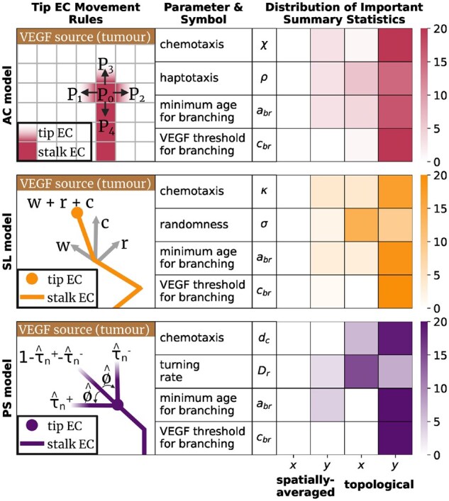 Figure 1
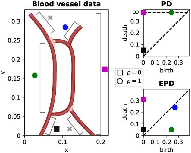 Figure 2
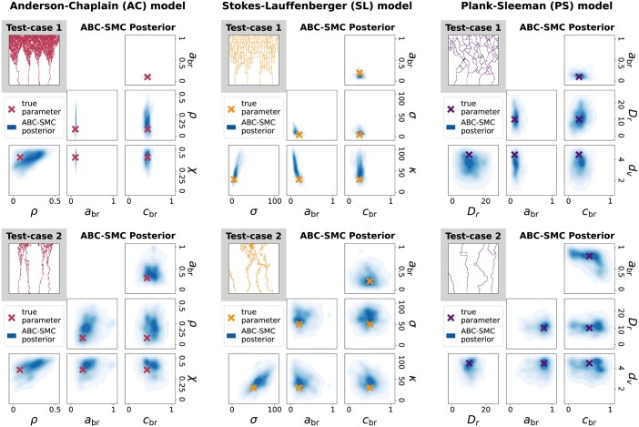 Figure 3
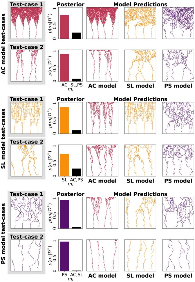 Figure 4
- —Engineering and Physical Sciences Research Council (EPSRC)
- —UK Centre for Topological Data Analysis EPSRC
- —Royal Society10.13039/501100000288
- —EPSRC10.13039/501100000266
Peer Reviews
No public reviews on file for this paper yet. If you reviewed it on a platform where reviews are public (OpenReview, ICLR, NeurIPS, ICML), you can paste yours below so the community can read it here.
Videos
No videos yet. Explain this paper in a talk, walkthrough, or lecture? Add one.
Taxonomy
TopicsMathematical Biology Tumor Growth · Angiogenesis and VEGF in Cancer · Gene expression and cancer classification
1 Introduction
Given multiple mathematical models which aim to reproduce the same biological data, determining which model and parameters give the best fit presents a theoretical and computational challenge. For example, spatio-temporal models often simulate complex high-dimensional data which is difficult to quantify and compare to observed data. Such models do not in general yield tractable likelihood functions, which significantly hinders the use of exact methods for parameter inference and model selection (Kirk et al. 2013).
Many mathematical models have been developed to study the mechanisms underlying tumour-induced angiogenesis (Scianna et al. 2013, Vilanova et al. 2017), a hallmark of cancer (Hanahan and Weinberg 2011). Tumour cells use chemical signals to stimulate the growth of new blood vessels from existing vasculature (Ferrara 2002), which provide a tumour mass with oxygen and nutrients that it requires to grow. However, instead of concise equations determining the growth of angiogenic networks, such models often comprise multiple agents and heterogeneous environments whose interactions depend non-deterministically on their spatial organization. Discrete models of tumour-induced angiogenesis, e.g. use multiple model rules and parameters to reproduce the branches, loops, and multiple components that characterize real vascular networks.
We use Topological Data Analysis (TDA), Approximate Bayesian Computation (ABC), and Random Forests (RFs) to develop a pipeline for parameter inference and model selection applicable to spatio-temporal models. TDA offers a toolkit of methods for quantifying spatial data (Ghrist 2008, Carlsson 2009, Edelsbrunner and Harer 2010). TDA has previously been used to study multi-agent temporal systems (Topaz et al. 2015, Bhaskar et al. 2019, Stolz et al. 2024) and was used in related work to compare models of insect locomotion (Ulmer et al. 2019) and pattern formation in zebrafish (Cleveland et al. 2023). ABC provides a statistical framework for using model simulations to approximate posterior distributions when likelihood functions are not available (Lintusaari et al. 2017). RFs are an ensemble estimation method from machine learning which have previously been combined with ABC to estimate parameter values (Raynal et al. 2019) and rank candidate models (Pudlo et al. 2016).
We begin by outlining three existing models of tumour-induced angiogenesis in which exact methods of parameter inference and model selection are not applicable. We show how TDA can be used to characterize spatial data simulated by the models and briefly describe methods from ABC and RF. We then present a three-step pipeline for parameter inference and model selection which we apply to the angiogenesis models. Commenting on the applicability of our pipeline to experimental data, we discuss how topological summaries may be used to evaluate a variety of modelling approaches in biology.
2 Model data and analysis
2.1 Angiogenesis models
Discrete models of tumour-induced angiogenesis simulate the movement of individual Endothelial Cells (ECs). Vascular Endothelial Growth Factors (VEGF) produced by tumour cells initiate a cascade of chemical reactions which drive ECs towards the tumour. Early models used the snail-trail model (Balding and McElwain 1985) in which tip ECs migrate up spatial gradients of VEGF and fibronectin, while stalk ECs proliferate in their path to produce a contiguous line of cells. When two separate trails of ECs meet they fuse together to form a loop, in a process known as anastomosis. A tip EC may also split into two tip ECs, which thereafter move independently. Migrating, branching and looping tip ECs eventually reach the tumour mass and the connecting trails of stalk ECs form a blood vessel network. Recent models reflect modern discoveries of cell mixing and phenotype switching (Stepanova et al. 2024), where ECs change type and overtake each other before forming a stable blood vessel network. Other models view ECs as a continuous population density rather than individual cells (Martinson et al. 2021) and account for blood flow and nutrient delivery when simulating vascular networks (Hormuth et al. 2021). We develop our pipeline of parameter inference and model selection on discrete angiogenesis models due to their simulation of finely resolved spatial data.
The Anderson-Chaplain (AC) (Anderson and Chaplain 1998), Stokes-Lauffenberger (SL) (Stokes et al. 1991), and Plank-Sleeman (PS) (Plank and Sleeman 2004) models use the snail-trail model to simulate movement of individual ECs in a 2D, square domain. We assume that VEGF levels increase from the bottom of the domain to a tumour at the top, guiding ECs to move upwards. Each model initializes multiple distinct tip ECs along the bottom of the domain, simulating their trajectories according to model-specific movement rules. In each model, we choose four parameters that are likely to lead to measurable changes in simulated data and we attempt to infer their values. Figure 1 illustrates the movement rules and model parameters in each model. See Section 1, available as supplementary data at Bioinformatics online for full statements of each model and its parameters.
In the AC model (Anderson and Chaplain 1998), a tip endothelial cell (EC) makes one of five possible moves on a square lattice in each time-step according to probabilities P0,P1,P2,P3,P4. A chemotaxis parameter χ biases movement probabilities in the direction of increasing VEGF concentration, and a haptotaxis parameter ρ biases moves in the direction of increasing fibronectin. In the SL model (Stokes et al. 1991), tip ECs move in any direction (off-lattice) with velocities modelled by a 2D stochastic differential equation. Parameters κ and σ determine how strongly an EC’s current velocity w is affected by the VEGF gradient c, and random variation r, respectively. The PS model (Plank and Sleeman 2004) assigns a constant speed to each tip EC and, at each time-step, rotates the angle that the velocity vector makes with the vertical. The probability τ^n++τ^n− that a tip EC turns by ϕ^ is determined by a turning rate parameter Dr. A chemotaxis parameter dc biases turns that re-orient the EC’s direction towards the tumour. In all models, a tip EC may bifurcate into two ECs which thereafter move independently if its age exceeds the minimum age for branching parameter abr and the VEGF concentration at its location exceeds the VEGF threshold for branching parameter cbr. We show how many spatially averaged and topological summary statistics, computed in either the x or y co-ordinate direction, appear among the 100 most important summary statistics to the inference of each parameter.
2.2 Data generation and analysis
Each angiogenesis model outlined in Section 2.1 (and described fully in Section 1, available as supplementary data at Bioinformatics online) simulates EC movement in a square domain. To summarize the spatial properties of each simulation, we overlay a regular grid onto the domain at the final timestep and compute a collection of spatially-averaged and topological summary statistics. For the spatially-averaged summary statistics, we compute the mean, standard deviation, minimum, maximum, range, and the 10th, 25th, 75th, and 90th percentiles of the x and y co-ordinates of EC locations in the grid. These were used in Nardini et al. (2021) to distinguish the AC model’s behaviour in different parameter regimes.
Persistent homology (PH) is a prominent method within Topological Data Analysis (TDA) (Ghrist 2008, Carlsson 2009, Edelsbrunner and Harer 2010) to quantify loops, branches, and connected components. Here, we require finer information than is provided by standard persistence; therefore, we use extended persistent homology (EPH) (Cohen-Steiner et al. 2009). We give an overview of PH and EPH, briefly indicating how EPH arises from PH and captures a greater range of spatial information within the angiogenesis data we simulate. See Section 2, available as supplementary data at Bioinformatics online for a full definition of EPH and a worked example.
To compute PH, a nested sequence of simplicial complexes, known as a filtration, is built on the data. Intuitively, a simplicial complex is a graph that includes nodes and edges as well as higher-order connections such as triangles or tetrahedra. A filtration must be carefully constructed such that each encodes the spatial properties of the underlying data at some spatial threshold defined by k. For example, Nardini et al. (2021) used a sweeping-plane filtration to analyse the AC model, where is constructed from those ECs which are a distance of k or more away from the tumour. Once a filtration has been chosen, one computes a sequence of -vector spaces known as homology groups. We use the field , which is widely adopted in applications for its simplicity and interpretability. Homology groups quantify p-dimensional topological features in each [see, e.g. Otter et al. (2017)]. detects connected components, detects loops and, in general, detects p-dimensional voids. We consider dimensions 0 and 1 only, since voids of dimension 2 or higher do not appear in the angiogenesis data we simulate. Persistence pairs are computed from the sequence of homology groups to quantify topological features in the filtration (Zomorodian and Carlsson 2005). A birth b corresponds to the index k in the filtration at which a topological feature first appears. A death d is either the index k at which the p-dimensional void it represents is filled in, or if the topological feature persists through the filtration. The difference is known as the persistence of a topological feature. The interpretation of in terms of the underlying data depends on the choice of filtration. In the sweeping-plane filtration used in Nardini et al. (2021), persistence pairs quantify connected components and loops in simulated vascular networks in terms of their distance from the tumour.
In PH, some topological features typically persist throughout the entire filtration. In Fig. 2, e.g. a connected component appears at and a loop at , and both persist for all values of y in the sweeping-plane filtration. The corresponding persistence pairs are therefore and , which quantify limited location information and no size information about the topological features they represent. Furthermore, PH computes one PD in each dimension ( and in this work), but we want to distinguish several different spatial structures (see Fig. 2 for examples).
A persistence diagram (PD) and extended persistence diagram (EPD) for a simple blood vessel computed using the vertical sweeping-plane filtration. The PD points quantify the size and location of the small lower branch (), and the locations of the component () and loop (). The EPD points quantify the location and size of all topological features quantified by the PD, in addition to the small upper branch (). The branches () are not detected by PH or EPH with this sweeping-plane filtration.
We would like to quantify the size and location of different spatial features. EPH provides this information by appending relative homology groups (Edelsbrunner and Harer 2010) to the sequence of ordinary homology groups in PH. Topological features which persist through all ordinary homology groups will die in the relative homology groups, so persistence pairs computed from EPH are guaranteed to have finite persistence. Each EPH persistence pair then be classified as one of four types depending on where the birth and death appear in the sequence of ordinary and relative homology groups, which provides additional information about the corresponding topological features. See Section 2, available as supplementary data at Bioinformatics online for a formal definition of topological feature types in EPH and their interpretation in simulated angiogenesis data. Figure 2 compares persistence pairs computed from a simple blood vessel network using PH and EPH, illustrating the extra information provided by EPH. We compute two extended persistence diagrams (EPDs) for each angiogenesis dataset–using a vertical and a horizontal sweeping-plane filtration. We vectorize each EPD using Persistence Images (Adams et al. 2017) and persistence statistics (Ali et al. 2023), and our topological summary statistics are the concatenation of these vectors.
3 Materials and methods
3.1 Approximate Bayesian computation
ABC provides a statistical framework for using data to infer model parameters. Suppose a model uses parameters to simulate data according to some probability distribution , called the likelihood. Parameter inference aims to determine the posterior distribution , which is the probability that parameters generated observed data . Using previous experiments or assumptions about feasible parameter values, one may define a prior distribution representing knowledge of the parameter values before data has been observed. The likelihood, prior and posterior are related by Bayes’ rule,
where the evidence is the integral over parameters in the support of the prior. Although Bayes’ rule gives a closed formula for the posterior distribution, it is often impractical to use directly. The likelihood function may be too complicated to derive for probabilistic spatial models in which many datasets may be simulated from the same parameters . Instead, Bayes’ rule is used to derive Approximate Bayesian Computation (ABC) algorithms (Lintusaari et al. 2017) which allow sampling from the posterior when the likelihood and evidence are not known. ABC algorithms sample candidate parameters from the prior and accept them if the distance between simulated and observed data is less than some tolerance for some distance function . If the tolerance is set to zero, then the distribution of accepted parameters is the posterior (Frazier et al. 2018). However, it is often not appropriate or possible to seek an exact posterior distribution from observed data, since a model may rarely reproduce observed data exactly, and the observed data may be noisy. It is therefore advisable to choose and such that parameter values are accepted if they simulate data that is similar to observed data. The general form of such a distance function is where and are vectors of summary statistics computed from model data and observed data respectively. Summary statistics aim to capture relevant properties of data as a low dimensional vector. As approaches 0, the distribution of parameters accepted by ABC algorithms approaches , which equals if the summary statistics are sufficient for the model in question, or is a close approximation if the summary statistics are insufficient but informative (Joyce and Marjoram 2008).
3.2 Random Forests
Random Forests (RFs) (Breiman 2001) learn relationships between feature vectors and response variables. Training data comprising a collection of feature vectors and corresponding response variables are used to train a RF, enabling it to predict the true response variable of an unseen feature vector . Regression RFs are used when are continuous values and classification RFs are used when are discrete labels. Raynal et al. (2019) used a regression RF for parameter inference by using simulated data to learn the relationship between summary statistics and parameter values . Given summary statistics of unseen data , the prediction predicts the true parameter value . In addition to predicting unseen feature vectors, a trained RF provides useful information about the training data. The out-of-bag prediction estimates the (known) response variable using pairs from the training data other than . The out-of-bag error rate then gives a (unbiased) measure of how well the relationship between and is captured by the rest of the training data. A trained RF also gives a measure of the importance of each co-variate j within feature vectors to the problem of predicting response variable . Intuitively, important features are those whose values within and differ when and do, and which are hence useful in learning the relationship between training data and .
3.3 Model selection
Given observed data , the model posterior gives the probability that models generated . ABC algorithms rely on the approximation , which holds as long as the vector carries a similar amount of information about the parameter value as the simulated data itself. However, the information loss suffered by a collection of summary statistics may vary between models (Robert et al. 2011), so it is inadvisable simply to infer as a (discrete) parameter using an ABC algorithm. Pudlo et al. (2016) instead used two RFs to approximate . A classification RF learns the relationship between simulated data and model label and gives a prediction of the model which generated unseen data . A regression RF is then trained to learn the relationship between and –the out-of-bag error rate of the classification RF. The regression RF is then used to estimate posterior probability as .
4 Spatial parameter inference and model selection
Given observed data , we wish to approximate the parameter posterior for candidate models and the model posterior . Informative summary statistics may be used to infer parameter values using ABC, but uninformative or poorly scaled summary statistics may misrepresent the difference between datasets generated by similar parameters (Blum et al. 2013). We therefore seek a collection of summary statistics that quantify simulated data and, in particular, quantify how simulated data changes when different model rules and parameters are used to generate it. We use informative summary statistics to approximate parameter and model posteriors in a three-step pipeline. We test this pipeline on toy models in Section 4, available as supplementary data at Bioinformatics online and apply it to the three angiogenesis models in Section 5.
Step 1: Identify informative summary statistics
We use RFs to find a small subset of summary statistics to be used in ABC. To generate training data, we draw parameter values from the prior distribution for each parameter in each model, simulate model data , and compute spatially averaged and topological summary statistics from the final simulated time-step. We train regression RFs to learn the relationship between summary statistics and parameter values –one RF for each parameter in each model. We then rank the spatially averaged and topological summary statistics by their importance according to the RF (see Section 3.2). In each RF, feature importance decreases exponentially [as in Raynal et al. (2019)] and a small subset of summary statistics provides most of the predictive power of each RF. We select an equal number of informative summary statistics from each RF, collecting a total of for each model. See Section 3, available as supplementary data at Bioinformatics online for a full definition of RF feature importance and a discussion of how we choose . RFs identify which summary statistics quantify the effect of each parameter on simulated data and allow us to omit those summary statistics which do not.
Step 2: Fit each model to the observed data
We use the summary statistics identified by step 1 to define a distance function for use in ABC. We use , where is the vector restricted to the top summary statistics identified in step 1, is computed from observed data, and the distance is averaged over multiple instances of observed data. We scale each summary statistic by the largest absolute value of that summary statistic in the training data. We then use the ABC-SMC algorithm of Del Moral et al. (2012) to approximate for each model. By using only those summary statistics which quantify the effect of parameter values on simulated data, we ensure is informative about the value of used to generate the observed data. Scaling ensures that each summary statistic contributes approximately equally to the distance function and limits the influence of poorly scaled summary statistics.
Step 3: Approximate the model posterior
Using summary statistics which are informative for all models, we use two more RFs to estimate the model posterior. Following Pudlo et al. (2016), we train a classification RF to learn the relationship between (unscaled) summary statistics and model indices in the training data. We modify to contain only those summary statistics which appear among the most important summary statistics for all models. We then train a regression RF to learn the relationship between and –the probability that the predicted model index is incorrect. The classification RF gives an estimate of the model that generated the observed data , and the regression RF is used to estimate as . We choose the value of in step 2 large enough to ensure that some informative summary statistics are selected for all three models under consideration–we use these to approximate the model posterior.
5 Results
5.1 RFs find small subsets of informative summary statistics
We sample n=10,000 model parameters from uniform priors with ranges taken from existing literature, or by analysing each model’s data generation rules (See Section 1, available as supplementary data at Bioinformatics online for details). We select summary statistics for each model and report the type of summary statistics selected—spatially averaged or topological, computed in the horizontal or vertical direction—in Fig. 1. A mixture of spatially averaged and topological summary statistics are selected for each parameter, however there is a clear preference for topological summary statistics for each parameter. In general, summary statistics computed in the vertical direction are selected more often than those computed in the horizontal direction, which is unsurprising, since most parameters regulate the movement of ECs upwards. However, the randomness parameter of the SL model and the turning coefficient of the PS model are two exceptions. These parameters cause ECs to deviate from their upward trajectory, and their inference therefore relies on topological summary statistics computed in the horizontal direction. No spatially averaged summary statistics computed in the horizontal (x) direction are chosen, indicating that these measures are too coarse to distinguish different model simulations.
5.2 ABC-SMC infers four parameters for each model and reproduces observed data
We create two test-cases for each model by simulating data at known parameter values 10 times. Each test-case exhibits quantitatively different vascular networks that each model can produce. Following steps 1 and 2 of Section 4, we use ABC-SMC to infer four parameters for each model and show the resulting approximate posteriors in Fig. 3. In each test-case, the approximate posterior is unimodal and encompasses the true parameter, often close to its densest part.
We infer the minimum age for branching (abr) and VEGF threshold for branching (cbr) in each model, as well as chemotaxis and haptotaxis parameters (χ and ρ) in the AC model, chemotaxis and randomness parameters (κ and σ) in the SL model, and chemotaxis and turning rate parameters (dc and Dr) in the PS model. We simulate each model 10 times at known parameter values to generate two synthetic test-cases for each model, and show the final time-step of one such simulation. We then use steps 1–2 of Section 3 to approximate the parameter posterior p(Θ|D) in each test-case. We project the approximate ABC-SMC posterior to each parameter pair and plot the resulting distributions (fitting a Gaussian kernel to the parameter values accepted in the final population of the ABC-SMC algorithm), along with the true parameter which generated the test-case.*
5.3 Random Forests correctly select models
Using step 3 of Section 4, we approximate the model posterior for each of the six test-cases. Fig. 4 shows the resulting approximate model posteriors, which identify the correct model with high probability in each test-case. We simulate each model at a parameter value drawn from its approximate parameter posterior and show the resulting ‘prediction’, which is a sample from the model’s approximation of the true data generating process. Each model generates data that is visually similar to the observed data, however we can identify the true model in each test-case.
We approximate the model posterior p(m|D) using the six test-cases from Fig. 3, highlighting one example of D*. For each test-case, we show one example of data simulated using an inferred parameter from each model’s approximate parameter posterior. Each ‘prediction’ shows an example of that model’s approximation of the true data generation process.*
6 Discussion
Using Topological Data Analysis (TDA) and Approximate Bayesian Computation (ABC), we have developed a pipeline for parameter inference and model selection applicable to complex spatial models. In previous work, TDA characterized the effect of two parameters in the AC model (Nardini et al. 2021) and was combined with ABC to infer them (Thorne et al. 2022). Here we extend this work by identifying a subset of informative summary statistics from multiple topological filtrations and use them to infer four parameters in three angiogenesis models using ABC-SMC. We further show how RFs can be used with TDA to approximate model posteriors and compare candidate models.
While we validated our pipeline using synthetic data simulated from angiogenesis models, previous studies used in vitro data to inform model rules and parameters (Milde et al. 2013, Connor et al. 2015, Vergroesen et al. 2025). The present work therefore enhances previous model analysis, since ABC provides a statistical framework for learning parameters and evaluating models, and TDA provides a variety of filtrations and vectorizations which may be adapted to different spatial data. In future work we will apply our pipeline to real experimental data, which will take the place of the synthetic test-cases in Figs 3 and 4 wherein the true parameter values and correct model will not be known.
In this study, we considered three models in which the paths traced by tip ECs form a static blood vessel network. Topological features, therefore, evolve monotonically in time in these models, and computing EPH at the final timestep was sufficient to infer parameters. In reality, sustained proliferation and vessel remodelling, where vasculature continually evolves after it is laid down, is characteristic of tumour-induced angiogenesis (Farnsworth et al. 2014). Indeed, vascular renormalization, in which vessel-targetting agents prune small or inefficient blood vessels, is a theorized treatment strategy (Magnussen and Mills 2021) aiming to temporarily enhance perfusion of the tumour to increase the effectiveness of radiotherapy (Jain 2014). Topological invariants that account for time-evolving data (Xian et al. 2022), directed flow networks (Chaplin et al. 2024) and multiparameter filtrations (Vipond 2020) could quantify such structural changes over time and be used to calibrate more sophisticated models. Rather than fixing the duration of simulations in these cases, simulation time could be an extra parameter to be inferred by our pipeline.
Although we specialized our pipeline to discrete models of tumour-induced angiogenesis, its flexibility allows application to a range of spatio-temporal models. Any summary statistic which quantifies the desired properties of simulated data would be identified by the RF in step 1 if it captures the effect of changing model parameters. In future, we will use our pipeline to systematically compare continuum, cell-based, agent-based, and discrete models by their ability to reproduce observed data.
Supplementary Material
btag065_Supplementary_Data
The reference list from the paper itself. Each links out to its DOI / PubMed record.
- 1Adams H , Emerson T, Kirby M et al Persistence images: a stable vector representation of persistent homology. J Mach Learn Res 2017;18:1–35.
- 2Ali D , Asaad A, Jimenez M-J et al A survey of vectorization methods in topological data analysis. IEEE Trans Pattern Anal Mach Intell 2023;45:14069–80.37647183 10.1109/TPAMI.2023.3308391 · doi ↗ · pubmed ↗
- 3Anderson AR , Chaplain MA. Continuous and discrete mathematical models of tumor-induced angiogenesis. Bull Math Biol 1998;60:857–99.9739618 10.1006/bulm.1998.0042 · doi ↗ · pubmed ↗
- 4Balding D , Mc Elwain DL. A mathematical model of tumour-induced capillary growth. J Theor Biol 1985;114:53–73.2409405 10.1016/s 0022-5193(85)80255-1 · doi ↗ · pubmed ↗
- 5Bhaskar D , Manhart A, Milzman J et al Analyzing collective motion with machine learning and topology. Chaos 2019;29:123125.31893635 10.1063/1.5125493 PMC 7027427 · doi ↗ · pubmed ↗
- 6Blum MGB , Nunes MA, Prangle D et al A comparative review of dimension reduction methods in approximate Bayesian computation. Stat Sci 2013;28:189–208.
- 7Breiman L. Random forests. Mach Learn 2001;45:5–32.
- 8Carlsson G. Topology and data. Bull Amer Math Soc 2009;46:255–308.