The Potential of Horizontal Wells for Aquifer Storage and Recovery in Saline Aquifers
Simon Kreipl, Mark Bakker, Boris M. van Breukelen

TL;DR
This study shows that horizontal wells can significantly improve water recovery in saline aquifers compared to vertical wells, especially under challenging buoyancy conditions.
Contribution
The study introduces horizontal wells as a novel solution to enhance aquifer storage and recovery in saline, low-transmissivity aquifers.
Findings
Horizontal wells achieved a median recovery efficiency of 45% after five cycles, outperforming vertical wells.
Vertical wells failed to recover freshwater under strong buoyancy conditions, while horizontal wells succeeded.
Dispersive mixing affected horizontal wells more but helped stabilize recovery in vertical wells.
Abstract
Aquifer Storage and Recovery (ASR) is a managed aquifer recharge method where water is injected and later extracted using wells. In saline aquifers, ASR performance is often limited by dispersive mixing, which creates a transition zone at the edge of the injected freshwater and buoyancy‐driven flow, which causes the freshwater to rise and deform during storage—both reducing recovery efficiency. This study investigates whether horizontal wells can improve ASR performance in saline, low‐transmissivity aquifers by achieving acceptable recovery efficiencies and outperforming conventional vertical wells. Three configurations were evaluated numerically with MODFLOW 6: a horizontal well, a fully penetrating vertical well, and a dual well system with a fully penetrating injection well and a partially penetrating extraction well. Models were tested on a large set of parameter combinations from…
Genes, proteins, chemicals, diseases, species, mutations and cell lines named across the full text — each resolved to its canonical identifier and authoritative record.
Click any figure to enlarge with its caption.
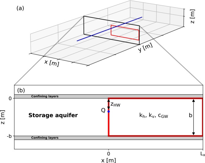 Figure 1
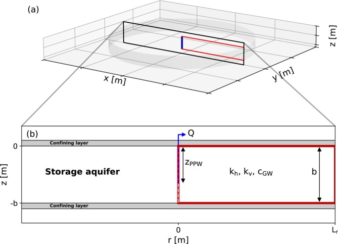 Figure 2
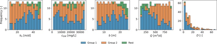 Figure 3
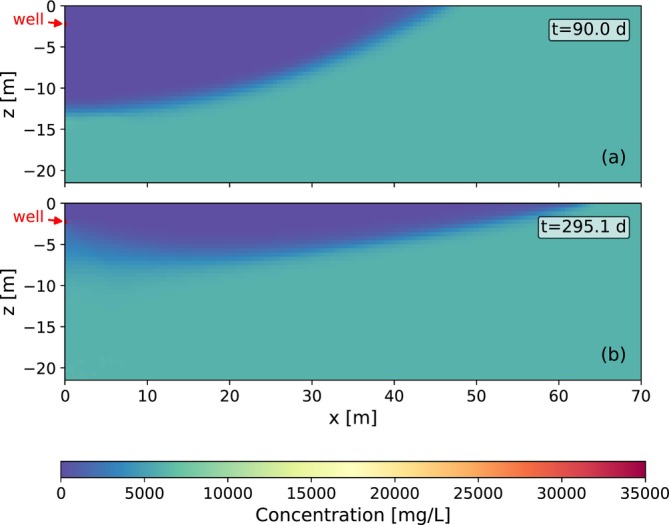 Figure 4
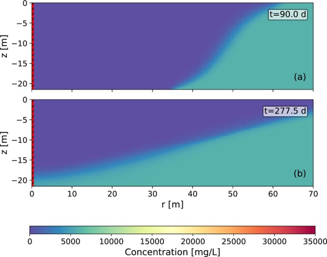 Figure 5
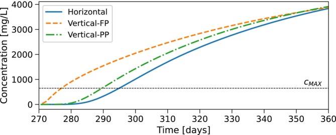 Figure 6
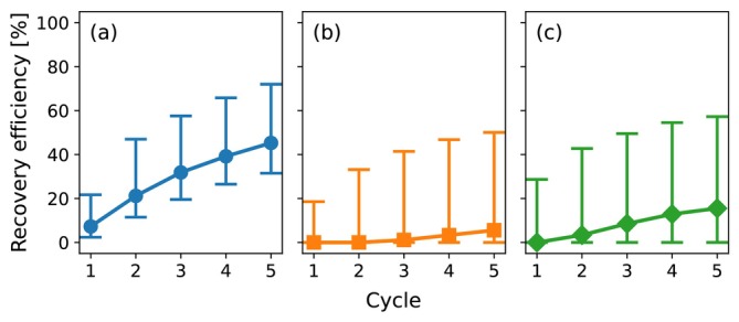 Figure 7
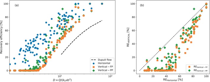 Figure 8
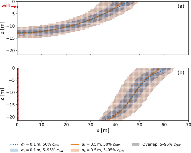 Figure 9
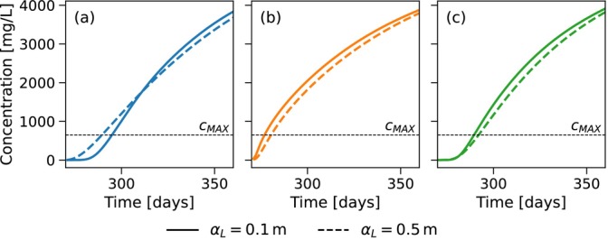 Figure 10
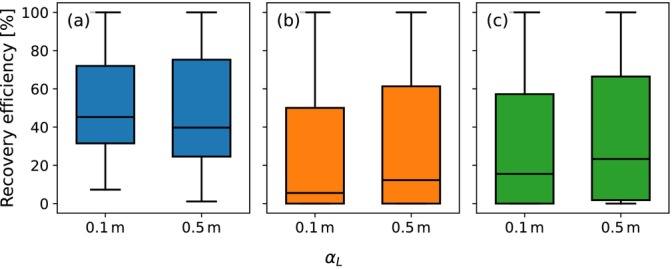 Figure 11
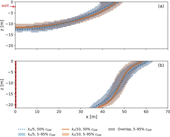 Figure 12
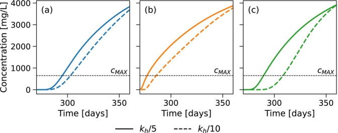 Figure 13
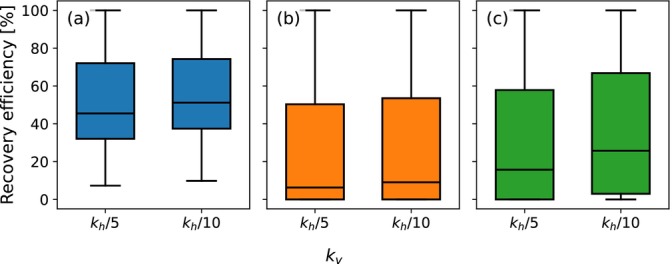 Figure 14
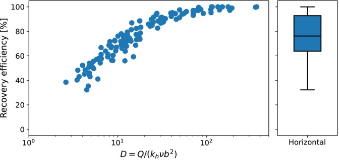 Figure 15
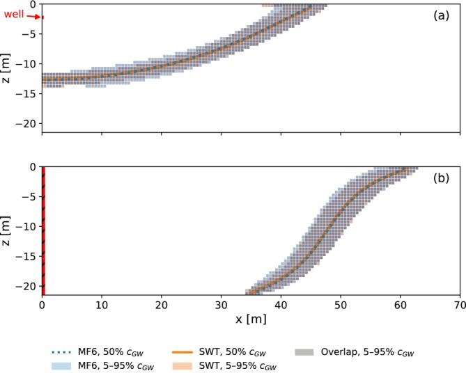 Figure 16
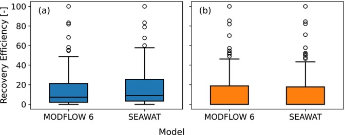 Figure 17
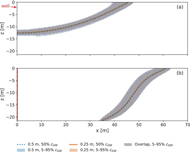 Figure 18
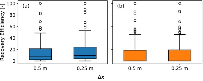 Figure 19
| Hydrogeological Conditions | Symbol | Unit | Value |
|---|---|---|---|
| Aquifer thickness | m | 5–25 | |
| Horizontal hydraulic conductivity | m/d | 10–50 | |
| Anisotropy ratio for conductivity | ‐ | 5 and 10 | |
| Background groundwater salinity | mg/L | 1000–35,000 | |
| Effective porosity | ‐ | 0.3 | |
| Longitudinal dispersivity | m | 0.1 and 0.5 | |
| Anisotropy ratio for dispersivity | ‐ | 0.1 | |
| Molecular diffusion | m2/d | ||
|
| |||
| Well radius | , | m | 0.25, 0.15 |
| Depth of horizontal well | m | 2 | |
| Length of horizontal well | m | 200 | |
| Depth of PPW | m | ||
| Well discharge | m3/d | 100–1000 | |
| Cycle length | d | 360 | |
| Injection period length | d | 90 | |
| Storage period length | d | 180 | |
| Injected freshwater concentration | mg/L | 0 | |
| Maximum extraction concentration | mg/L | 650 | |
| Flow and Transport Solver Settings | Symbol | Value |
|---|---|---|
| Maximum outer iterations |
| 30 |
| Maximum inner iterations |
| 100 |
| Head change convergence criterion (outer) |
| m |
| Head change convergence criterion (inner) |
| m |
| Linear acceleration method |
| “BICGSTAB” |
| Relaxation factor |
| 0.97 |
|
| ||
| Advection solver |
| TVD |
| Courant number |
| 1.4 |
|
| ||
| Model domain length in | , | 1024.80, 1025.05 |
| Well domain length in | , | 100 |
| Vertical cell size | 0.5 m | |
| Number of layers | ||
| Horizontal cell size | , | 0.5 m |
| Number of horizontal cells | 294 | |
| Number of well cells | 1 (Horizontal) | |
| (FP) | ||
| (PP) | ||
| Parameter | Symbol | Value |
|---|---|---|
| Aquifer thickness | 21.5 m | |
| Horizontal hydraulic conductivity | 41.7 m/d | |
| Background groundwater salinity | 6,100 mg/L | |
| Well discharge | 522.9 m3/d | |
| ‐value | 6.06 |
- —Nederlandse Organisatie voor Wetenschappelijk Onderzoek10.13039/501100003246
Peer Reviews
No public reviews on file for this paper yet. If you reviewed it on a platform where reviews are public (OpenReview, ICLR, NeurIPS, ICML), you can paste yours below so the community can read it here.
Videos
No videos yet. Explain this paper in a talk, walkthrough, or lecture? Add one.
Taxonomy
TopicsGroundwater flow and contamination studies · Groundwater and Isotope Geochemistry · Enhanced Oil Recovery Techniques
Introduction
Groundwater resources are facing depletion in many parts of the world. Managed aquifer recharge offers a valuable solution by enhancing groundwater recharge and storage through human intervention (Dillon et al. 2019; Scanlon et al. 2023). Aquifer Storage and Recovery (ASR) is one type of managed aquifer recharge, where wells are used for the injection and extraction of water. In ASR, water is stored in times of surplus, for later recovery during times of scarcity. In temperate climate zones, such as in the Netherlands, ASR can be used to store excess precipitation in winter, for times of increased demand in dryer summers. In the coastal regions of the Netherlands, brackish and saline aquifers are often the only available and technically feasible storage zones for ASR. Although generally less favorable, applications of ASR in brackish and saline aquifers have been reported (van Ginkel et al. 2014; Zuurbier et al. 2014; Maliva et al. 2020).
A typical ASR cycle consists of three phases: injection, storage, and extraction, each characterized by specific flow and transport processes. During injection, the ambient groundwater is displaced by the recharged water, forming a bubble of freshwater around the well. Dispersive mixing creates a transition zone at the edges of the bubble, with a salinity gradient from freshwater to saline groundwater (Esmail and Kimbler 1967; Ward et al. 2007). In the storage phase, the freshwater bubble deforms due to buoyancy‐driven flow, as the lighter freshwater tends to rise and float on top of the denser groundwater (Ward et al. 2007; Bakker 2010). During extraction, flow reverses and the freshwater bubble contracts as water is withdrawn. Extraction is usually terminated when the extracted water concentration exceeds a specific water quality threshold such as a salinity limit. The recovery efficiency—defined as the percentage of injected water that can be recovered to meet this threshold—is an important metric to evaluate the performance of ASR systems.
The recovery efficiency is higher for high injection volumes, and low hydraulic conductivity, aquifer thickness, and groundwater salinity. These are the key variables that govern buoyancy‐driven flow (e.g., Merritt 1986; Lowry and Anderson 2006; Bakker 2010). A high hydrodynamic dispersion, as a proxy for small‐scale aquifer heterogeneity, increases mixing between water sources. Generally, a wider mixing zone leads to an earlier breakthrough of saltwater during extraction, which reduces the recovery efficiency (e.g., Merritt 1986; Lowry and Anderson 2006; Maliva et al. 2020). A wider mixing zone can also attenuate buoyancy‐driven flow and stabilize the freshwater bubble. This can lead to a net increase in recovery efficiency under some conditions (Ward et al. 2007).
One method to mitigate the adverse impacts of buoyancy‐driven flow is the use of multiple partially penetrating wells (Zuurbier et al. 2014, 2016; Witt et al. 2021). This technique involves using multiple wells within a single borehole, each screened at different depths. When the deeper wells begin to salinize as the fresher water floats upwards, they are successively deactivated, while the shallower wells continue extracting the fresher water. This way, Zuurbier et al. (2014) were able to increase the recovery efficiency from between 15% and 30% to 40% for agricultural use.
The hydraulic conductivity and aquifer thickness (i.e., transmissivity) also determine how much pressure is exerted on the aquifer during injection. If the transmissivity is too low, excessive pressure poses the risk of fracturing confining layers. This limits the range of feasible injection rates for the ASR operation. The infiltrated water then needs to be distributed over multiple wells.
Horizontal directionally drilled wells, initially developed in the oil‐and‐gas industry, were introduced to the groundwater sector for contaminated site remediation in the 1990s (Houben et al. 2022). They have since been used for mine dewatering (Struzina et al. 2011), abstraction of potable water (Sass and Treskatis 2000a, 2000b), and managed aquifer recharge (Zuurbier et al. 2015; Perdikaki et al. 2022). A valuable advantage of these wells is that the injection pressure is distributed over a larger area, making it less pronounced (Steward and Jin 2003). This makes horizontal wells particularly beneficial in low‐transmissivity aquifers, where much greater water volumes can be infiltrated and extracted from a single well, avoiding the need for multiple vertical wells (Beljin and Losonsky 1992; Sass and Treskatis 2000a, 2000b). Additionally, a more evenly distributed drawdown during freshwater extraction in saline aquifers reduces upconing of the fresh‐saltwater interface, increasing the volume of extractable water (Stoeckl and Houben 2012; Pauw et al. 2016).
Currently, horizontal directionally drilled wells may be installed with high positional accuracy (Licht et al. 2001). Nevertheless, horizontal wells remain technically more complex to construct than vertical wells, particularly in unconsolidated sediments. The installation of an effective gravel pack along the horizontal section is challenging. In addition, drilling fluids are typically required to stabilize the borehole during drilling, which necessitates extensive well development and increases the likelihood of skin formation (Houben et al. 2022). Horizontal wells also generally require higher initial capital investment due to the increased complexity of drilling operations and the limited availability of specialized drilling contractors. However, these higher installation costs may be offset by higher well yields and the potential to replace multiple vertical wells with a single horizontal well. In cases where one horizontal well substitutes several vertical wells, system‐level operational costs may be reduced due to the use of a single pump and simplified associated conveyance infrastructure, resulting in lower power supply requirements.
Despite their potential advantages, the application of horizontal wells in ASR is sparsely researched. A first application for agricultural water supply involved installing two superimposed wells, each 70 m in length (Zuurbier et al. 2015). A shallow well, positioned within a freshwater lens in a brackish coastal aquifer, injected and extracted water. A deeper well, positioned below the freshwater lens, continuously extracted brackish water to counteract upconing during freshwater extraction from the shallow well, and maintain the position of the fresh–saltwater interface during the ASR operation. Under these specific conditions, horizontal wells showed promising results (Zuurbier et al. 2015).
These findings suggest that horizontal wells could facilitate ASR installations in conditions previously considered infeasible, particularly low‐transmissivity aquifers. Furthermore, horizontal wells may achieve higher recovery efficiencies in saline aquifers because they may reduce the effects of buoyancy‐driven flow and reduce upconing. However, the flow and transport processes that govern the performance of horizontal well ASR systems have not yet been investigated. Additionally, no studies have compared the recovery efficiency of horizontal well ASR systems with conventional vertical wells.
This study investigates the potential of horizontal wells for ASR in saline aquifers, particularly under conditions where vertical wells do not perform well. The objective is to assess whether horizontal wells can achieve operationally acceptable recovery efficiencies in such settings and to identify if and when they may offer advantages over vertical wells. The study aims to develop a generalized understanding of how buoyancy‐driven flow and dispersive mixing influence ASR performance through numerical modeling of density‐dependent groundwater flow and solute transport.
Methods
This study employs numerical modeling of density‐dependent groundwater flow and solute transport to evaluate the potential advantages and limitations of horizontal wells for ASR in saline aquifers. Simulations are performed on a conceptual groundwater system comprising of a homogeneous storage aquifer, confined above and below by horizontal, impermeable layers. The aquifer is characterized by its thickness b, horizontal and vertical hydraulic conductivity kh and kv, and a background groundwater salinity cGW, expressed as total dissolved solids (TDS). Changes in aquifer storage due to compressibility (specific storage) are neglected. Transport processes are governed by the aquifer's effective porosity neff, longitudinal and transversal dispersivity αL and αT, and molecular diffusion Dm.
Two separate models are developed: one representing a horizontal well and the other one a vertical well. The horizontal well is LHW long, as presented in Figure 1a. For this study, a two‐dimensional vertical cross‐section is simulated, as shown in Figure 1b; tip effects are not considered here. The well has a radius rHW and is positioned near the top of the storage aquifer at a depth zHW. The conceptual model of the vertical well system is depicted in Figure 2a. A radial cross‐section is simulated, as shown in Figure 2b. The well has a radius rVW. Two configurations of the vertical well system are analyzed: (i) A fully penetrating vertical well (Vertical‐FP) which fully penetrates the aquifer thickness, facilitating both injection and extraction through the same well; (ii) a partially penetrating vertical well (Vertical‐PP) which is a dual‐well configuration comprising of a fully penetrating injection well and a partially penetrating extraction well. The latter extends from the top of the aquifer to a depth zPPW. Both wells are in the same location and are screened in the same borehole.
(a) Three‐dimensional conceptual model of an infinitely long horizontal well; (b) Two‐dimensional cross‐section along x‐direction of a slice of the horizontal well. The blue pipe represents the horizontal well. The red box represents the domain of the numerical model.
(a) Three‐dimensional conceptual model of a vertical well; (b) Radial cross‐section through the center of the vertical well. The blue pipe represents the vertical well. The red box represents the domain of the numerical model.
Multiple ASR cycles of 360 days (tCYCLE) are simulated, each comprising of three main phases: a 90 day injection phase (tINJ) during which freshwater with a TDS concentration cFW is injected; a 180 day storage phase (tSTO); and an extraction phase that continues as long as the TDS concentration of the extracted water cEXT remains below a predefined maximum threshold cMAX=650mg/L—a value commonly used for potato irrigation. Once this limit is reached, the system enters an idle phase until the start of the next cycle. If the limit is not reached, extraction stops after 90 days. The discharge from the well Q is identical during the injection and extraction phases. For the horizontal well model, the well discharge is divided over the length of the horizontal well as QHW=Q/LHW. The performance of the respective systems is evaluated based on the recovery efficiency, defined as the percentage of injected water with a concentration less than cMAX that can be recovered. Numerical values for the hydrogeological conditions and design and operation choices are summarized in Table 1.
Numerical Model
Numerical modeling of groundwater flow and solute transport was conducted using MODFLOW 6, Version 6.6.1. (Hughes et al. 2017). MODFLOW 6 enables coupling of a groundwater flow model (Langevin et al. 2017) with a solute transport model (Langevin et al. 2022). Density‐dependent flow is incorporated using the BUY‐package (Langevin et al. 2020), which accounts for buoyancy effects. Advection is simulated using a second‐order Total Variation Diminishing (TVD) scheme. Model development, running, and post‐processing were carried out using the FloPy Python package (Bakker et al. 2016). Computationally intensive simulations were performed on the DelftBlue Supercomputer (DHPC 2022).
The model for the horizontal well system is shown in Figure A1. One half of the flow domain is simulated to reduce computational effort. The well is positioned at x=0m, where a no‐flow boundary is applied. The horizontal well is simulated with the MODFLOW WEL‐package and is represented using a single model cell. The model for the vertical well system is shown in Figure A2. An axisymmetric model is used for the vertical well as described by Langevin (2008). The well is positioned at r=0m. The vertical well is simulated using the MODFLOW Multi‐Aquifer‐Well‐package (MAW), where the specified well discharge is distributed by maintaining a hydrostatic hydraulic head over the connected MAW‐cells. For both system types, the upper and lower boundaries of the model are defined as no‐flow boundaries and a constant‐head (CHD) boundary with h=0m is applied at the outer model edges Lx and Lr, which are sufficiently distant to avoid influencing the simulation results.
Rectangular grid cells are used for both models. A refined grid is used in the vicinity of the well—referred to here as the well domain—extending up to a distance of Lx,WD and Lr,WD, respectively. This region is discretized using uniform cells with a width of Δx and Δr. For the horizontal well model, the first column of cells in the x‐direction has a width of Δx/2 because only half of the domain is modeled. Beyond the well domain, horizontal cell sizes increase gradually by a factor of 1.05 to reduce computational demand while maintaining accuracy. Vertically, the aquifer is discretized into layers with a uniform thickness of Δz. The time step size Δt is dynamically adjusted during the simulation to satisfy a Courant number of 1.4, with a maximum allowable step size of 1 day. The parameters used in the numerical model are summarized in Table 2.
Selection of Parameter Sets
The effect of six parameters on ASR performance is investigated: aquifer thickness b, horizontal hydraulic conductivity kh, background groundwater salinity cGW, well discharge Q, longitudinal dispersivity αL (while αT=0.1αL), and vertical anisotropy of the hydraulic conductivity kh/kv. The first four parameters are varied over a range for one value of αL and kh/kv, after which simulations are repeated with the same set of parameters but a different value of αL and a different value of kh/kv. Parameter sets of the four varied parameters are based on the parameter D introduced by Bakker (2010) as
where ν is the density difference ratio [−] as
where ρGW and ρFW are the density of the background groundwater and injected freshwater, respectively [kg/m3]. The density of groundwater is obtained from the salinity using the approximate formula
where ρFW=1000kg/m3 and ∂ρ/∂C is the density slope which for the range from freshwater to seawater is approximated as 0.734 for concentrations in TDS. Note that all computations are done in kg/m3, but the concentrations are reported as mg/L in this paper.
The parameter D incorporates the key variables that influence buoyancy‐driven flow. Low values of D are associated with lower recovery efficiencies, while higher values—resulting, for example, from higher discharge rates or lower hydraulic conductivity, background salinity, or aquifer thickness—tend to yield higher recovery efficiencies. In this study, D is used as a proxy for buoyancy‐driven flow. By varying the parameters that comprise D, the influence of buoyancy on the recovery efficiency of the horizontal and vertical well models is investigated. The recovery efficiencies reported by Bakker (2010) are based on a Dupuit interface model for a vertical well which did not take into account dispersive mixing or vertical anisotropy of the hydraulic conductivity. For Dupuit interface flow, the recovery efficiency is a function only of the parameter D and of the relative lengths of the injection, storage, and recovery periods. In this study, the effect of mixing and vertical anisotropy of the hydraulic conductivity on the recovery efficiency is investigated.
The analysis is focused on low‐transmissivity aquifers where vertical wells do not perform well. The ranges of the varied parameters are selected to reflect these conditions. The horizontal hydraulic conductivity values range from 10 to 50 m/d for fine‐ to medium‐grained sands (Domenico and Schwartz 1990). Aquifer thickness values range from 5 to 25 m to represent relatively thin aquifers. The background groundwater salinity range is from 1000 to 35,000 mg/L TDS, covering the spectrum from brackish to seawater. The total injection and extraction rates range from 100 to 1000 m3/d. For the horizontal well model, the discharge is distributed uniformly along the well. For the vertical well model, the discharge is distributed uniformly along the well screen so that the pressure is hydrostatic in the well.
A total of 250 parameter sets are generated using Latin Hypercube Sampling (McKay et al. 1979) based on the ranges specified in Table 1 (with αL=0.1m and kv=kh/5). The parameter sets are filtered using the following three constraints to avoid parameter combinations that are not physically plausible or do not align with the scope of this investigation:
- D‐value: D>1
- Transmissivity: T=khb<1000m2/d
- Injection pressure: s<5m
Parameter sets with D<1 are excluded because buoyancy effects are considered too large. Sets with T>1000m2/d are excluded to focus the study on hydraulically restricted aquifers. Finally, sets with s>5m are removed due to the risk of fracturing confining layers. The injection pressure is calculated for a single, fully penetrating vertical well following Theis (1935) (e.g., as presented in Bakker and Post 2022), with a specific storage coefficient (Ss) of 10−4m−1.
The frequency distributions of the four varied input variables as well as parameter D are shown in Figure 3. The frequency of each parameter is roughly evenly distributed across the specified range. The D‐values resulting from the generated parameter sets are predominantly low: 136 out of 250 samples result in D<10. This indicates that, given the input ranges, most combinations correspond to scenarios with relatively strong buoyancy‐driven flow and potentially lower recovery efficiencies. Of 250 sets, 236 meet the D‐value constraint. As has been discussed, this constraint excludes combinations of low well discharge and high hydraulic conductivity, background salinity, or aquifer thickness. Of 250 sets, 242 meet the transmissivity constraint. This constraint excludes combinations of high aquifer thickness and hydraulic conductivity. Of 250 sets, 128 meet the injection pressure constraint. This constraint excludes parameter sets with high well discharge combined with low aquifer thickness and hydraulic conductivity. Two groups of parameter sets are created. The blue bars show the frequency distributions of the first group of parameter sets that meet all three constraints. This group contains 109 parameter sets. The orange bars show the frequency distribution of the second group of parameter sets that meet only the D‐value and transmissivity constraint but not the injection pressure constraint. This group contains 122 sets consisting mainly of combinations of high well discharge and low aquifer thickness and hydraulic conductivity. The green bars show the frequency distribution of the remainder of the original 250 parameter sets that do not meet any of the constraints.
Frequency distribution of parameters. Group 1: Parameter sets that meet all three constraints (n1=109). Group 2: Parameter sets that meet D‐value and transmissivity constraints but not the injection pressure constraint (n2=122). Rest: Parameter sets that do not meet any constraints.
The first group of parameter sets represents the subset of physically plausible scenarios that align with the scope of this investigation. These parameter sets are used as input variables for the horizontal and vertical well models to assess whether horizontal wells can achieve operationally feasible recovery efficiencies and to identify if and when they offer advantages over vertical wells. These simulations are repeated once with αL increased from 0.1 to 0.5 m, and once for kv reduced from kh/5 to kh/10. The second group of parameter sets is used as input variables for only the horizontal well model because the injection pressure is too high for a vertical well. Finally, two additional investigations are performed on the first group of parameter sets to evaluate how the simulation results are effected by more accurate solutions. This includes (i) a comparison with a model that uses a higher order TVD‐scheme for the simulation of advective transport, and (ii) a comparison with a finer grid resolution to reduce numerical dispersion. In some of the investigations, one or two simulations failed to converge for the vertical well configuration. These cases were excluded across all well configurations to ensure consistency, and the analysis was performed on the remaining successful simulations.
Results and Discussion
Flow and Transport Dynamics
The flow and transport dynamics of an ASR system are illustrated using a representative example simulation for the first ASR cycle in a brackish aquifer. The parameters of the selected example simulation are listed in Table 3.
During ASR, the injection of freshwater displaces ambient groundwater, forming a freshwater bubble around the well. A mixing zone develops between the injected freshwater and the background groundwater. A cross‐section of the concentration distribution of the example simulation is shown in Figure 4 for the horizontal well and in Figure 5 for the vertical well. Concentrations are presented at (a) the end of injection and (b) the end of extraction (when cEXT=cMAX), respectively. With the horizontal well, the injected freshwater moves downward and outward, forming a horizontally stretched semi‐cylinder. Over time, buoyancy effects push the freshwater further outward at the aquifer top. Upward migration is limited by the presence of an impermeable cover layer. With the vertical well, the freshwater spreads radially, forming a cylindrical bubble. Over time, buoyancy effects cause upward migration of the freshwater, tilting the vertical sides of the cylinder. This leads to an extended bubble radius at the aquifer top and a reduced radius at the bottom.
Concentration distribution for a horizontal well (a) at the end of injection (after 90 days) and (b) at the end of extraction (when cEXT=cMAX) for the example simulation. Due to symmetry, only one half of the flow domain is shown. The red area with the black lines on the left of the figure is the well cell (an annotation arrow labeled “well” indicates its position).
Concentration distribution for a fully penetrating vertical well (a) at the end of injection (after 90 days) and (b) at the end of extraction (when cEXT=cMAX) for the example simulation. A radial cross‐section is shown. The red area with black lines on the left of the figure is the well.
During extraction, flow reverses and the freshwater bubble contracts as water is withdrawn. The extracted concentrations during the first ASR cycle of the example simulation with the horizontal well and the fully and partially penetrating vertical wells are shown in Figure 6. The concentration begins to rise as the mixing zone reaches the well. For the horizontal well, saltwater is drawn toward the well through upconing, which leads to a continued increase in concentration. Extraction is terminated when the average concentration of extracted water exceeds cMAX. Residual freshwater remains in the upper part of the aquifer. For the example in Figure 6, this occurs after 295.1 days (25.1 days of extraction), yielding a recovery efficiency of 27%. For the fully penetrating vertical well, saltwater first reaches the well at the bottom due to the reduced bubble radius. For the example in Figure 6, extraction is stopped after 277.5 days, resulting in a recovery efficiency of 7%. For the partially penetrating well, the end of extraction is delayed from 277.5 to 290 days as compared to the fully penetrating well, improving recovery efficiency from 7% to 22%.
Extracted water concentration during the first ASR cycle for the example simulation. Extraction starts at 270 days. Vertical wells show the flux weighted average concentration across the respective well cells; horizontal wells show concentration from the single well cell.
Recovery Efficiencies
The simulations for the horizontal well and the fully and partially penetrating vertical wells were repeated for the first group of parameter sets over five ASR cycles. The progression of recovery efficiency across these cycles is presented in Figure 7 for (a) the horizontal well, (b) the fully penetrating vertical well, and (c) the partially penetrating vertical well. The markers represent the median recovery efficiency, while the whiskers represent the interquartile range. Initial recovery efficiencies are low for all systems: the horizontal well starts at a median recovery efficiency of 7% compared to 0% for both vertical well configurations. Recovery efficiency increases with each cycle. This trend results from unrecovered water that remains in the aquifer and becomes available for extraction in subsequent cycles. Recovery efficiency increases until a balance is reached between extractable water and residual storage, at which point a system specific maximum is reached. After five cycles, the horizontal well achieves a median recovery efficiency of 45%, while the fully and partially penetrating vertical wells reach 6% and 16%, respectively. These values are conservative due to the selection of a long storage period (180 days) and a low CMAX of 650 mg/L. Shorter storage durations or a higher CMAX will improve recovery efficiency across all systems, while the differences between systems are unlikely to change significantly.
Progression of the recovery efficiency over five ASR cycles. (a) is the horizontal well, (b) is the fully penetrating vertical well, and (c) is the partially penetrating vertical well. Markers indicate the median per cycle; whiskers show the interquartile range.
The recovery efficiency after five cycles is shown in Figure 8 for all of the parameter sets of the first group. The recovery efficiency is plotted as a function of the parameter D in Figure 8a. The line marked as “Dupuit flow” refers to the recovery efficiency from the Dupuit interface flow model (Bakker 2010). The recovery efficiency of the horizontal well is compared to the fully and partially penetrating vertical well in Figure 8b. The recovery efficiency is lowest for small D‐values. Among the 50 scenarios with D < 4, the horizontal well achieves a median recovery efficiency of 33%, while the median of the fully and partially penetrating vertical wells is 0%. This highlights the potential of horizontal wells to provide viable recovery under conditions where vertical wells are ineffective. The recovery efficiency increases with D across all configurations until a maximum of 100% is reached. The difference between the horizontal well and the fully and partially penetrating vertical wells decreases with a higher general recovery efficiency.
Recovery efficiency after five ASR cycles. (a) is the recovery efficiency as a function of parameter D. “Dupuit flow” refers to recovery efficiency from the Dupuit interface flow model (Bakker 2010). (b) is a comparison of recovery efficiencies of the horizontal well with the fully and partially penetrating vertical wells.
Significant variability in recovery efficiency is observed for similar D‐values, especially with horizontal wells. This variability arises from the dual role of groundwater salinity: it affects both the density difference (captured in D with the density difference ratio, ν) as well as the degree of mixing at the fresh–saltwater interface (not captured in D). Mixing with a higher salinity groundwater increases the concentration of extracted water more rapidly and yields a lower recovery efficiency compared to another parameter set with a lower groundwater salinity but a similar D‐value because of a higher aquifer thickness or hydraulic conductivity or a lower total discharge.
Effect of Dispersivity
The simulations of the first group of parameter sets are repeated to investigate the effect of the dispersivity on the ASR simulations. The dispersivity is a model parameter that captures the influence of heterogeneity on solute transport and governs mixing between injected freshwater and ambient groundwater. The longitudinal dispersivity is increased from αL=0.1m to 0.5m. A comparison of the mixing zones at the end of injection for the example simulation of Table 3 is given in Figure 9. Both the result for (a) the horizontal well and (b) the fully penetrating vertical well are shown. In these figures, the shaded areas represent 5%–95% concentration of background groundwater, which serve as indicators of the mixing zone width. As expected, the mixing zone becomes wider with increased dispersivity for both systems. The blue and orange contours represent the 50% concentration. A comparison of the contours of the vertical well shows that the interface is slightly more tilted at the aquifer top and bottom when the dispersivity is smaller. This suggests that a wider mixing zone (i.e., larger dispersivity) attenuates the interface tilting process, consistent with findings reported by Ward et al. (2007).
Comparison of mixing zones at the end of injection (t = 90 days) for αL=0.1m and 0.5m for the example simulation. (a) is the horizontal well and (b) is the fully penetrating vertical well. Shaded area shows 5%–95% concentration of background groundwater, while colored curves represent the 50% contour. The shaded area for αL=0.5m completely overlaps the shaded area for αL=0.1m in this case.
A comparison of the extracted water concentration during the first ASR cycle for the example simulation of Table 3 with the two dispersivities is shown in Figure 10 for (a) the horizontal well, (b) the fully penetrating vertical well, and (c) the partially penetrating vertical well. For the horizontal well, extraction is terminated earlier at 289.8 days for αL=0.5m compared to 295.1 days for αL=0.1m, resulting in a decrease in recovery efficiency from 27% to 22%. This reduction is primarily attributed to the earlier arrival of the saltwater front, driven by the wider mixing zone. In the case of the fully and partially penetrating vertical well, extraction ends slightly later at 281.5 days instead of 277.5 and 292.2 days instead of 290 days, increasing recovery efficiency from 7% to 11% and from 22% to 24%. Here, the earlier saltwater arrival is counter‐balanced by the attenuated interface tilting, resulting in a net increase in recovery efficiency.
Comparison of the extracted water concentration during the first ASR cycle for αL=0.1m and αL=0.5m for the example simulation. (a) is the horizontal well, (b) is the fully penetrating vertical well, and (c) is the partially penetrating vertical well. Extraction starts at 270 days. Vertical wells show flux weighted average concentration across the respective well cells; horizontal well shows concentration from the single well cell.
Boxplots comparing the recovery efficiencies of the two dispersivity values after five ASR cycles for the simulated parameter sets of the first group are shown in Figure 11 for (a) the horizontal well, (b) the fully penetrating vertical well, and (c) the partially penetrating vertical well. For the horizontal well, the 75th percentile recovery efficiency increases slightly from 72% to 75%. In contrast, the median and 25th percentile decrease from 45% to 40% and from 32% to 25%, respectively. These results suggest that while high‐efficiency scenarios remain relatively unaffected by increased mixing, the majority experience a decline in recovery efficiency due to the earlier arrival of the concentration front. For the fully penetrating vertical well, the 25th percentile remains constant at 0%. The median and 75th percentile show increases from 6% to 12% and from 50% to 61%. For the partially penetrating vertical well, the 25th percentile, median, and 75th percentile increase from 0% to 2%, 16% to 23%, and from 57% to 66%, respectively. These trends indicate that vertical wells generally benefit from increased mixing, due to the attenuating effect of a broader mixing zone on interface tilting. In conclusion, an increased degree of dispersive mixing reduces the difference in recovery efficiency between horizontal and vertical well systems.
Boxplots of the recovery efficiencies after five ASR cycles for αL=0.1m and αL=0.5m. (a) is the horizontal well, (b) is the fully penetrating vertical well, and (c) is the partially penetrating vertical well.
Effect of Anisotropy
The simulations of the first group of parameter sets are repeated to investigate the effect of the vertical anisotropy of the hydraulic conductivity on the ASR simulations. The vertical hydraulic conductivity is reduced from kv=kh/5 to kh/10. A comparison of the mixing zones at the end of injection for the example simulation of Table 3 is given in Figure 12. Both the results for (a) the horizontal well and (b) the fully penetrating vertical well are shown. For the horizontal well, it is evident that the freshwater bubble under kv=kh/10 extends further laterally but penetrates less deep than in the kv=kh/5 case. This behavior results from the reduced vertical hydraulic conductivity, which constrains downward movement and promotes horizontal spreading of the freshwater bubble. For the vertical well, the interface tilting under kv=kh/10 is less pronounced as compared to kv=kh/5. This is also attributed to the lower vertical hydraulic conductivity which attenuates interface tilting.
Comparison of mixing zones at the end of injection (t = 90 days) for kv=kh/5 and kv=kh/10 for the example simulation. (a) is the horizontal well and (b) is the fully penetrating vertical well. Shaded area shows 5%–95% concentration of background groundwater, while colored curves represent the 50% contour.
A comparison of the extracted water concentration during the first ASR cycle for the example simulation of Table 3 with the two anisotropy values is shown in Figure 13 for (a) the horizontal well, (b) the fully penetrating vertical well, and (c) the partially penetrating vertical well. For the horizontal well, the extraction period is extended from 295.1 days for kv=kh/5 to 303.1 days for kv=kh/10, resulting in an increase in recovery efficiency from 27% to 36%. For the fully and partially penetrating vertical well, the extraction period is extended from 277.5 to 286.6 days and from 290 to 308.5 days, with recovery efficiency rising from 7% to 17% and from 22% to 42%, respectively. Across all well configurations, the higher anisotropy (kv=kh/10) limits vertical flow, thereby reducing the influence of buoyancy. This improves the recovery efficiency by maintaining a more stable freshwater bubble.
Comparison of the extracted water concentration during the first ASR cycle for kv=kh/5 and kv=kh/10 for the example simulation. (a) is the horizontal well, (b) is the fully penetrating vertical well, and (c) is the partially penetrating vertical well. Extraction starts at 270 days. Vertical wells show flux weighted average concentration across the respective well cells; horizontal well shows concentration from the single well cell.
Boxplots comparing the recovery efficiencies of the two anisotropy values after five ASR cycles for the simulated parameter sets of the first group are shown in Figure 14 for (a) the horizontal well, (b) the fully penetrating vertical well, and (c) the partially penetrating vertical well. For the horizontal well, the 25th percentile and median recovery efficiencies increase from 32% to 37% and from 46% to 51%, respectively. The 75th percentile shows a marginal increase from 72% to 74%. These results suggest that the improvements at higher anisotropies are more pronounced in low‐efficiency scenarios, where buoyancy effects are more significant. For the fully penetrating vertical well, the 25th percentile remains unchanged at 0%, while the median and 75th percentile increase from 6% to 9% and from 50% to 54%, respectively. For the partially penetrating vertical well, the 25th, median, and 75th percentiles increase from 0% to 3%, 16% to 26%, and 58% to 67%, respectively. These trends indicate consistent improvements for all of the ASR systems. This improvement is primarily due to the restriction of vertical flow, which mitigates buoyancy‐driven flow.
Boxplots of the recovery efficiencies after five ASR cycles for kv=kh/5 and kv=kh/10. (a) is the horizontal well, (b) is the fully penetrating vertical well, and (c) is the partially penetrating vertical well.
High Pressure Conditions
The parameter sets in the second group meet the D‐value and transmissivity constraints, but not the injection pressure constraint. These scenarios are only simulated with the horizontal well model because the injection pressure is too high for the vertical well. Alternatively, the storage volume can be distributed over multiple vertical wells. The number of wells, their spatial configuration and the distance between the wells become critical design parameters for such cases, and is beyond the scope of this investigation.
The recovery efficiency after five ASR cycles is shown in Figure 15 as a function of parameter D as well as a boxplot. The median D‐value of this group of parameter sets is 14.3 (25th percentile = 8.5; 75th percentile = 39.9), which is higher than the median D‐value of 4.6 in the first group (25th percentile = 2.6; 75th percentile = 10.6). The median recovery efficiency is 76% with a 25th percentile of 64% and 75th percentile of 93%. This demonstrates the potential of horizontal wells to achieve high recovery efficiencies in high pressure conditions where a single vertical well is not possible.
Recovery efficiency of the horizontal well simulations after five ASR cycles for the second group of parameter sets which meet the D‐value and transmissivity constraint, but not the injection pressure constraint. Recovery efficiency is shown as a function of parameter D and as a boxplot.
More Accurate Solutions
The simulations of the first group of parameter sets are repeated for two additional investigations to determine whether a more accurate solution changes the recovery efficiency significantly: (i) application of a higher‐order TVD scheme for advective transport as implemented in SEAWAT, and (ii) refinement of the model grid to reduce numerical dispersion. The influence of these enhancements on the simulation results is discussed below. A detailed comparison of simulation runtimes is provided in Appendix B (Figures B1 and B2) for MODFLOW 6 and SEAWAT, and in Appendix C (Figure C1) for the varying model grid sizes.
SEAWAT, Version 4 (Guo and Langevin 2002; Langevin et al. 2008) employs a third‐order TVD scheme, in contrast to the second‐order scheme employed in MODFLOW 6. SEAWAT requires some different solution parameters, which are provided in Table B1. A comparison of the mixing zones at the end of injection for the example simulation of Table 3 is given in Figure 16, for (a) the horizontal well and (b) the fully penetrating vertical well. Despite identical model parameters, the mixing zone is slightly wider in the MODFLOW 6 simulation. This is likely caused by the lower order TVD scheme in MODFLOW 6, which causes greater numerical dispersion.
Comparison of mixing zones at the end of injection (t = 90 days) for second‐order TVD (MODFLOW 6) and third‐order TVD (SEAWAT) for the example simulation. (a) is the horizontal well and (b) is the fully penetrating vertical well. Shaded area shows 5%–95% concentration of background groundwater, while colored curves represent the 50% contour.
Boxplots comparing the recovery efficiencies of the MODFLOW 6 and SEAWAT simulations after one ASR cycle for the simulated parameter sets of the first group are shown in Figure 17 for (a) the horizontal well and (b) the fully penetrating vertical well. For the horizontal well, the median and 75th percentile increase slightly from 7% and 22% with MODFLOW 6 to 9% and 26% with SEAWAT. For the vertical well, the median stays constant at 0% and the 75th percentile decreases slightly from 19% to 18%. The differences in recovery efficiency are small and don't influence the conclusions of this investigation.
Boxplots of the recovery efficiency after one ASR cycle using second‐order TVD (MODFLOW 6) and third‐order TVD (SEAWAT). (a) is the horizontal well and (b) is the fully penetrating vertical well.
Next, the first ASR cycle is repeated with smaller cell sizes; both simulations are conducted with MODFLOW 6. The general model setup for the refined model grid investigation remains as described previously, with cell dimensions reduced from Δx=Δr=Δz=0.5m to 0.25m in the well domain. No other model parameters changed. Using a refined grid reduces numerical dispersion and improves accuracy, particularly in simulating relatively sharp concentration fronts. A comparison of the mixing zones for the original and the refined grids for the example simulation of Table 3 is given in Figure 18 for (a) the horizontal well and (b) the fully penetrating vertical well. For consistency, concentration data from the original grid is re‐projected onto the refined grid. The mixing zone is slightly wider with the original (coarser) grid due to increased numerical dispersion.
Comparison of mixing zones at the end of injection (t = 90 days) for the original grid (Δx=0.5m) and the refined grid (Δx=0.25m) for the example simulation. (a) is the horizontal well and (b) is the fully penetrating vertical well. Shaded area shows 5%–95% concentration of background groundwater, while colored curves represent the 50% contour. For the comparison the concentration data from the original grid is re‐projected onto the refined grid.
Boxplots comparing recovery efficiencies of the different model grids after one ASR cycle for the simulated parameter sets of the first group are shown in Figure 19 for (a) the horizontal well and (b) the fully penetrating vertical well. For the horizontal well, the median and 75th percentile increase from 7% and 21% with Δx=0.5m to 10% and 24% with Δx=0.25m. For the vertical well, the median and 75th percentile stay at 0% and 19%, respectively. These differences are minor and do not affect the overall conclusions of this study.
Boxplots of the recovery efficiency after one ASR cycle with the original grid (Δx=0.5m) and the refined grid (Δx=0.25m). (a) is the horizontal well and (b) is the fully penetrating vertical well.
Conclusions
This study investigated the potential of horizontal wells for ASR in saline, low‐transmissivity environments where vertical wells are typically ineffective. The objective was to assess whether horizontal wells can achieve operationally feasible recovery efficiencies under these conditions and to determine the circumstances under which they may offer advantages over conventional vertical wells.
Numerical simulations showed that horizontal wells generally achieved significantly higher recovery efficiencies than vertical wells across the range of investigated conditions. The performance differences were primarily governed by density‐driven flow and dispersive mixing, which influence the movement and stability of the injected freshwater bubble. After five ASR cycles, horizontal wells yielded a median recovery efficiency of 45%, compared to 6% and 16% for fully and partially penetrating vertical wells, respectively. These are conservative values; higher values are obtained for shorter storage durations and/or a higher CMAX, allowing for longer extraction. For agricultural use, even fairly low efficiencies can have a significant effect on crop production and improve water security in regions facing seasonal shortages. The advantage of horizontal wells was most pronounced under strong buoyancy conditions (D < 4), where horizontal wells recovered a median of 33% while vertical wells mostly failed to recover any freshwater. However, increased dispersive mixing reduces horizontal well performance by accelerating saltwater breakthrough while modestly improving vertical well recovery by stabilizing flow near the fresh–saltwater interface. Groundwater salinity plays a dual role, influencing both buoyancy and mixing. This introduces greater variability in horizontal well performance compared to vertical wells. It was also demonstrated that horizontal wells can achieve high recovery efficiencies under high‐pressure conditions, offering a viable alternative when vertical wells are constrained by injection pressure limits.
These results underscore the potential of horizontal wells to extend ASR to hydrogeologically challenging settings, particularly saline aquifers with low transmissivity. It is recommended to consider horizontal wells in the planning of ASR systems when the hydraulic conditions require multiple vertical wells, and when buoyancy‐driven flow significantly limits vertical well performance—especially under strong buoyancy (D < 4) and generally for D < 10. Despite these advantages, horizontal wells remain more technically complex and costly to construct, which presently limits their widespread implementation. Moreover, their sensitivity to groundwater salinity demands precise design and adaptation of the well orientation, depth, and length to account for spatial salinity variability.
This study used idealized, two‐dimensional models to develop a generalized understanding of horizontal well performance in ASR systems. As such, it does not account for several site‐specific factors that can influence recovery efficiency, including non‐uniform flow along the horizontal well, background groundwater flow, aquifer heterogeneity, and vertical leakage through confining layers. The modeling framework was limited to a simplified representation of multiple partially penetrating wells. Future investigations may incorporate fully three‐dimensional representations of horizontal wells to capture the full flow dynamics and explore the effects of these complexities. Further research into optimized configurations of multiple vertical wells, including well spacing and placement strategies, will also provide valuable comparisons for ASR system design.
Author's Note
The author does not have any conflicts of interest or financial disclosures to report.
The reference list from the paper itself. Each links out to its DOI / PubMed record.
- 1Bakker, M. 2010. Radial Dupuit interface flow to assess the aquifer storage and recovery potential of saltwater aquifers. Hydrogeology Journal 18, no. 1: 107–115. 10.1007/s 10040-009-0508-1 · doi ↗
- 2Bakker, M. , and V.E.A. Post . 2022. Analytical Groundwater Modeling: Theory and Applications Using Python, 1st Edition. London: CRC Press. 10.1201/9781315206134. · doi ↗
- 3Bakker, M. , V.E.A. Post , C.D. Langevin , J.D. Hughes , J.T. White , J.J. Starn , V. Post , and M.N. Fienen . 2016. Scripting MODFLOW model development using python and Flo Py. Groundwater 54, no. 5: 733–739. 10.1111/gwat.12413 27027984 · doi ↗ · pubmed ↗
- 4Beljin, M.S. , and G. Losonsky . 1992. HWELL: A Horizontal Well Model. Colorado, USA: International Groundwater Modeling Center and the Association of Groundwater Scientists and Engineers.
- 5DHPC . 2022. Delft Blue supercomputer (phase 1). https://www.tudelft.nl/dhpc/ark/Delft Blue Phase 1
- 6Dillon, P. , P. Stuyfzand , T. Grischek , M. Lluria , R.D.G. Pyne , R.C. Jain , J. Bear , J. Schwarz , W. Wang , E. Fernandez , C. Stefan , M. Pettenati , J. van der Gun , C. Sprenger , G. Massmann , B.R. Scanlon , J. Xanke , P. Jokela , Y. Zheng , R. Rossetto , M. Shamrukh , P. Pavelic , E. Murray , A. Ross , J.P. Bonilla Valverde , A. Palma Nava , N. Ansems , K. Posavec , K. Ha , R. Martin , and M. Sapiano . 2019. Sixty years of global progress in managed aquifer · doi ↗
- 7Domenico, P.A. , and F.W. Schwartz . 1990. Physical and Chemical Hydrogeology. New York: John Wiley & Sons.
- 8Esmail, O.J. , and O.K. Kimbler . 1967. Investigation of the technical feasibility of storing fresh water in saline aquifers. Water Resources Research 3, no. 3: 683–695. 10.1029/WR 003i 003p 00683 · doi ↗