Classification of driver and passenger mutations in different cancer types using deep neural networks
Medha Pandey, Anoosha Paruchuri, M Michael Gromiha

TL;DR
This study uses deep learning to classify driver and passenger mutations in 30 cancer types, improving accuracy with structural data from AlphaFold.
Contribution
A novel deep learning method integrating AlphaFold structures to distinguish driver from passenger mutations in cancer.
Findings
Motif-based preferences and structural features improve driver mutation classification.
The model achieved 84.06% accuracy using 10-fold cross-validation.
AlphaFold integration enhanced pathogenicity prediction of mutations.
Abstract
Cancer is driven by genetic changes, known as mutations, that lead to the uncontrolled division of cells. The functional significance of a vast number of these cancer somatic mutations is unknown, and it is one of the major challenges in cancer research. In this study, we performed an integrative analysis of 30 tumor types from PAN-cancer mutation data collected from the COSMIC database. We have analyzed a set of 61 364 missense mutations (57 535 drivers and 3829 passengers) from 682 cancer-causing genes and derived various important features from amino acid sequences, predicted AlphaFold structures, and amino acid contact networks. We observed that the motif-based preference, neighboring residue information, residue depth, and disorder regions around the site of mutation are important for the discrimination of drivers and passengers. We further developed cancer-specific computational…
Genes, proteins, chemicals, diseases, species, mutations and cell lines named across the full text — each resolved to its canonical identifier and authoritative record.
Click any figure to enlarge with its caption.
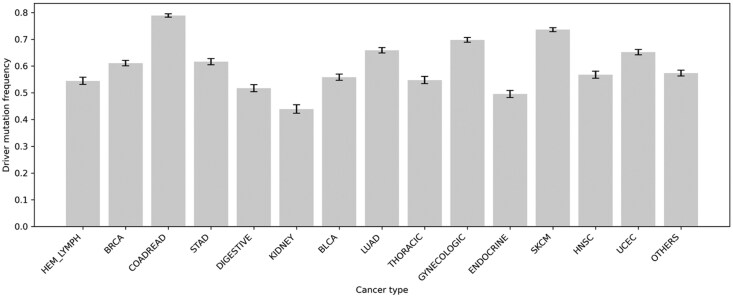 Figure 1
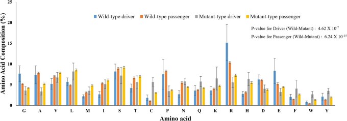 Figure 2
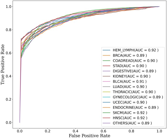 Figure 3
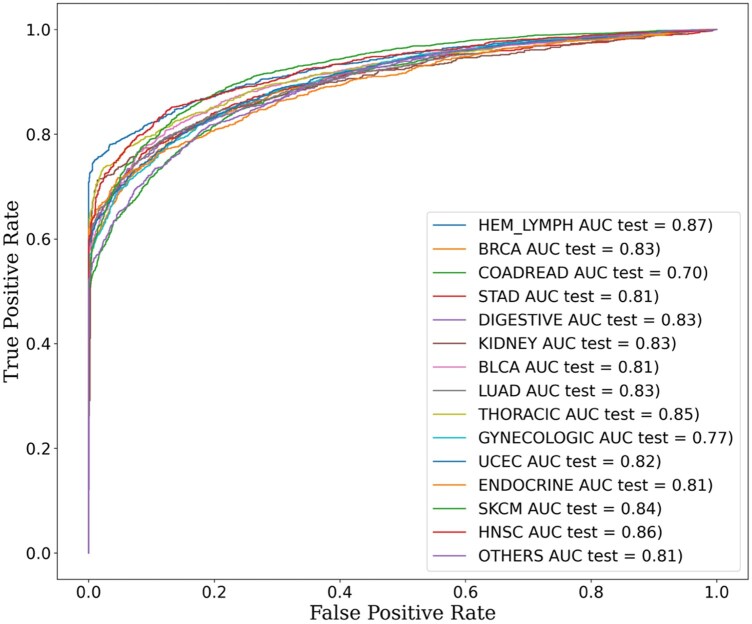 Figure 4
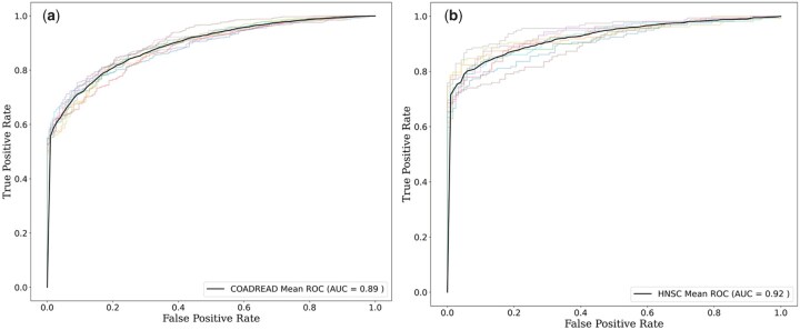 Figure 5
| Groups | Performance on training and 10-fold cross-validation | |||||
|---|---|---|---|---|---|---|
| Sensitivity (%) | Specificity (%) | Accuracy (%) | Balanced accuracy (%) | AUC | MCC | |
| Hem.Lymph | 89.26 (82.39) | 85.95 (84.76) | 87.30 (83.49) | 87.11 (83.57) | 0.87 (0.92) | 0.74 (0.68) |
| BRCA | 83.51 (82.40) | 83.23 (76.42) | 83.40 (80.07) | 83.37 (79.41) | 0.83 (0.89) | 0.67 (0.62) |
| COADREAD | 81.33 (94.05) | 84.15 (46.54) | 81.93 (84.01) | 82.74 (70.30) | 0.83 (0.90) | 0.57 (0.47) |
| STAD | 83.78 (83.55) | 86.66 (77.29) | 84.89 (81.15) | 85.22 (80.42) | 0.85 (0.90) | 0.69 (0.61) |
| Digestive | 87.76 (77.13) | 74.55 (85.40) | 81.38 (81.13) | 81.16 (81.27) | 0.81 (0.89) | 0.63 (0.63) |
| Kidney | 73.97 (78.30) | 98.99 (90.72) | 88.00 (85.27) | 86.48 (84.51) | 0.86 (0.90) | 0.77 (0.71) |
| BLCA | 84.88 (79.71) | 85.30 (85.51) | 85.30 (85.51) | 85.07 (82.27) | 0.85 (0.91) | 0.70 (0.65) |
| LUAD | 88.29 (82.35) | 80.57 (79.24) | 85.66 (81.28) | 84.43 (80.79) | 0.84 (0.90) | 0.61 (0.61) |
| Thoracic | 77.03 (81.33) | 95.29 (83.30) | 85.29 (82.22) | 86.16 (82.31) | 0.86 (0.90) | 0.72 (0.65) |
| Gynecologic | 86.98 (84.49) | 77.24 (70.94) | 84.10 (80.39) | 82.22 (77.71) | 0.81 (0.89) | 0.63 (0.55) |
| Endocrine | 86.34 (88.00) | 75.24 (66.34) | 83.03 (81.45) | 80.79 (77.17) | 0.81 (0.89) | 0.60 (0.56) |
| SKCM | 94.42 (91.26) | 68.01 (68.85) | 87.45 (85.35) | 81.22 (81.06) | 0.81 (0.92) | 0.66 (0.62) |
| HNSC | 90.21 (83.71) | 83.69 (85.60) | 87.39 (84.53) | 86.95 (84.66) | 0.87 (0.92) | 0.74 (0.61) |
| UCEC | 95.19 (83.27) | 58.61 (52.98) | 82.46 (80.92) | 76.90 (79.89) | 0.77 (0.90) | 0.60 (0.60) |
| Others | 69.81 (79.03) | 94.22 (79.63) | 80.21 (79.28) | 82.02 (79.33) | 0.82 (0.89) | 0.64 (0.52) |
|
|
|
|
|
|
|
|
| Groups | Performance on training and 10-fold cross-validation | ||||||
|---|---|---|---|---|---|---|---|
| Sensitivity | Specificity | Accuracy | Balanced accuracy (%) | AUC | MCC | PR-AUC | |
| (%) | (%) | (%) | |||||
| Hem.Lymph | 88.97 | 82.66 | 86.09 | 85.81 | 0.87 | 0.72 | 0.95 |
| BRCA | 81.1 | 82.26 | 81.55 | 81.68 | 0.83 | 0.62 | 0.94 |
| COADREAD | 80.74 | 81.68 | 80.94 | 81.21 | 0.7 | 0.54 | 0.97 |
| STAD | 80.5 | 82.93 | 81.43 | 81.71 | 0.81 | 0.62 | 0.94 |
| Digestive | 86.99 | 70.13 | 78.85 | 78.56 | 0.83 | 0.58 | 0.92 |
| Kidney | 72.42 | 98.07 | 86.8 | 85.24 | 0.83 | 0.74 | 0.93 |
| BLCA | 84.04 | 83.97 | 84.01 | 84 | 0.81 | 0.68 | 0.95 |
| LUAD | 84.9 | 77.35 | 82.33 | 81.13 | 0.83 | 0.61 | 0.96 |
| Thoracic | 74.09 | 92.88 | 82.59 | 83.49 | 0.85 | 0.67 | 0.94 |
| Gynecologic | 87.17 | 74.44 | 83.32 | 80.8 | 0.77 | 0.61 | 0.96 |
| Endocrine | 94.83 | 51.51 | 72.97 | 73.17 | 0.81 | 0.51 | 0.92 |
| SKCM | 93.66 | 63.45 | 85.68 | 78.55 | 0.84 | 0.61 | 0.97 |
| HNSC | 88.76 | 79.95 | 84.95 | 84.36 | 0.86 | 0.69 | 0.95 |
| UCEC | 93.57 | 55.72 | 80.4 | 74.65 | 0.82 | 0.55 | 0.96 |
| Others | 67.29 | 93.31 | 78.38 | 80.3 | 0.81 | 0.61 | 0.93 |
| Overall | 83.94 | 78.02 | 82.02 | 80.98 | 0.82 | 0.62 | 0.95 |
| UniProt ID | Gene name | Driver | Passenger | Sensitivity | Specificity | Accuracy |
|---|---|---|---|---|---|---|
| PTPRD | 1276 | – | 85.99 | – | – | |
| P53 | 1215 | 315 | 90.66 | 85.39 | 88.32 | |
| MUC4 | 793 | 135 | 81.50 | 82.96 | 81.66 | |
| SMCA4 | 681 | 105 | 83.77 | 73.33 | 82.73 | |
| DICER | 568 | 90 | 83.85 | 77.78 | 83.19 | |
| VGFR3 | 561 | 210 | 86.47 | 80.48 | 85.11 | |
| ASXL1 | 539 | 555 | 78.13 | 85.04 | 81.31 |
| No of mutations | No of proteins | Drivers | Passengers | Sensitivity | Specificity | Accuracy |
|---|---|---|---|---|---|---|
| 1 | 21 | 21 | – | 85.71 | – | 85.71 |
| 2–10 | 142 | 776 | 318 | 86.34 | 73.90 | 82.72 |
| 11–20 | 78 | 1175 | 898 | 86.21 | 73.61 | 80.75 |
| 21–30 | 49 | 1257 | 1216 | 85.36 | 77.88 | 81.68 |
| 31–40 | 26 | 940 | 989 | 85.53 | 80.08 | 82.74 |
| 41–50 | 29 | 1383 | 1572 | 84.60 | 81.93 | 83.18 |
| 51–60 | 24 | 1441 | 1152 | 83.07 | 84.38 | 83.65 |
| 61–70 | 22 | 1550 | 1005 | 85.74 | 84.78 | 85.36 |
| 71–80 | 15 | 1283 | 1276 | 87.61 | 81.27 | 84.45 |
| 81–90 | 17 | 1569 | 1487 | 83.94 | 71.15 | 77.72 |
| 91–100 | 11 | 1140 | 908 | 85.35 | 81.61 | 83.69 |
| >100 | 205 | 62935 | 32263 | 85.25 | 82.92 | 84.46 |
| Cancer group | Number of proteins | Number of driver mutations | Number of predicted drivers | Comparison with other methods | ||
|---|---|---|---|---|---|---|
| FATHMM-cancer | LIST-S2 | PROVEAN | ||||
| BRCA | 11 | 23 | 19 (82.60) | 15 (65.21) | 17 (73.91) | 17 (73.91) |
| SKCM | 5 | 15 | 13 (86.66) | 9 (60) | 8 (53.33) | 7 (46.67) |
| LUAD | 30 | 49 | 45 (91.83) | 30 (61.22) | 23 (49.94) | 23 (49.94) |
| Digestive | 3 | 11 | 6 (54.54) | 8 (72.72) | 3 (27.27) | 5 (45.45) |
| Gynecologic | 39 | 61 | 49 (80.32) | 38 (62.29) | 30 (49.18) | 45 (73.77) |
| Thoracic | 6 | 36 | 31 (86.11) | 27 (75) | 23 (63.89) | 20 (55.55) |
| Others | 52 | 88 | 79 (89.77) | 61 (69.31) | 61 (69.32) | 59 (67.04) |
| Name | Computational method | Sensitivity | Specificity | Accuracy | Balanced accuracy |
|---|---|---|---|---|---|
| SIFT | Probabilistic; sequence homology; alignment | 62.54 | 58.11 | 60.32 | 60.33 |
| MutationTaster | Naïve Bayes classifier | 86.17 | 33.55 | 61.10 | 59.86 |
| FATHMM | Hidden Markov Model | 35.45 | 53.90 | 44.06 | 44.67 |
| MutationAssessor | Conservation-based statistical model | 82.66 | 33.52 | 59.27 | 58.09 |
| PROVEAN | Alignment-based delta score | 53.94 | 67.29 | 60.12 | 60.62 |
| VEST4 | Random forest | 73.30 | 45.71 | 60.04 | 59.51 |
| MetaSVM | Support vector machine | 38.56 | 71.96 | 54.15 | 55.26 |
| MetaLR | Logistic regression | 40.90 | 67.40 | 53.22 | 54.15 |
| MetaRNN | Recurrent neural network | 60.37 | 60.62 | 60.36 | 60.49 |
| M-CAP | Gradient boosting | 76.55 | 29.29 | 54.13 | 52.92 |
| DEOGEN2 | Gradient boosting | 46.46 | 64.10 | 54.56 | 55.28 |
| LIST-S2 | Logistic regression (Ensemble) | 74.90 | 47.29 | 61.73 | 61.10 |
| MutPred | Random forest | 52.98 | 62.33 | 57.18 | 57.65 |
| MVP | Deep neural network | 78.96 | 32.60 | 56.33 | 55.78 |
| MPC | Bayesian/statistical score | 78.44 | 55.12 | 67.19 | 66.78 |
| Polyphen2 | Naïve Bayes classifier | 68.38 | 52.19 | 60.80 | 60.28 |
| REVEL | Random forest; Ensemble; score from multiple predictors | 41.92 | 65.16 | 52.81 | 53.54 |
| LRT | Likelihood ratio test | 71.53 | 47.15 | 60.43 | 59.34 |
| CADD | Support vector machine | 96.98 | 9.90 | 54.85 | 53.44 |
| FATHMM_MKL | Multiple kernel learning | 89.62 | 21.42 | 57.56 | 55.52 |
| FATHMM-XF | Extreme boosting (XGBoost) | 72.95 | 54.46 | 64.78 | 63.71 |
| DANN | Deep neural network; genomic annotations | 96.72 | 10.36 | 54.91 | 53.54 |
| AlphaMissense | Deep neural network; protein language model; AlphaFold based | 86.11 | 59.23 | 70.00 | 72.67 |
| Present method | Deep neural network; protein sequence, structure, and network based |
|
|
|
|
- —Department of Biotechnology, Government of India
Peer Reviews
No public reviews on file for this paper yet. If you reviewed it on a platform where reviews are public (OpenReview, ICLR, NeurIPS, ICML), you can paste yours below so the community can read it here.
Videos
No videos yet. Explain this paper in a talk, walkthrough, or lecture? Add one.
Taxonomy
TopicsCancer Genomics and Diagnostics · Bioinformatics and Genomic Networks · Genomics and Rare Diseases
1. Introduction
Cancer is a leading cause of death worldwide, accounting for nearly 10 million deaths or one in six deaths. The most common cancers include breast, lung, colon, rectum, and prostate. Cancer statistics collected from the American Cancer Society suggest that the mortality rate due to cancer has decreased since 1991, but specific cancers, such as breast, prostate, and uterine cancer, have increased in incidence, which needs to be addressed (Siegel et al. 2023). Due to advancements in large-scale genomics and parallel sequencing technologies, a huge number of somatic mutations in various cancer types have become a powerful resource. These mutations with detailed clinical information are stored in major databases including The Cancer Genome Atlas (TCGA) (Weinstein et al. 2013), International Cancer Genome Consortium (ICGC) (Jennings and Thomas 2016), Database of Curated Mutations in cancer (DoCM) (Ainscough et al. 2016), and Catalogue Of Somatic Mutations In Cancer (COSMIC) (Tate et al. 2019). Various studies have utilized these large-scale mutation data for systematic analysis of cancer mutations, which is necessary to explore the preferred patterns of somatic mutations at the genome (Bozic et al. 2010, Abecasis et al. 2012, Iengar 2012, Kandoth et al. 2013, Vogelstein et al. 2013, Rentzsch et al. 2019, Oh and Sung 2021) and proteome levels (Mao et al. 2013, Anoosha et al. 2016, Pejaver et al. 2020, Pandey et al. 2022). While these analyses have provided insights into the complex landscape of mutations in cancer cells, the interpretation of individual mutations has not yet been completely explored. One of the key challenges is to identify functional mutations (drivers) from a large group of biologically neutral or non-functional mutations (passengers).
Several methods have been developed to identify functional/pathogenic mutations in various diseases (Thomas et al. 2006, Yue et al. 2019, Alabi et al. 2020, Tan et al. 2021, Lin et al. 2023) as well as specific to cancer (Tokheim and Karchin 2019, Chen et al. 2020, Pandey et al. 2022, Vyatkin et al. 2022). Anoosha et al. (2015) developed a supervised machine-learning model using support vector machines to discriminate cancer driver mutations from passengers, and the method is specific to the epidermal growth factor receptor (EGFR) protein, one of the most important targets in cancer. Pandey et al. (2022) proposed a machine-learning method to classify driver and passenger mutations associated with glioblastoma. Recently, deep learning has gained attention for its ability to handle large datasets and to provide more accurate predictions (Angermueller et al. 2016, Luo et al. 2019, Rogers et al. 2020, Liao et al. 2021, Ko et al. 2022).
Investigations have been carried out for individual proteins such as P53 and BRAF by integrating cancer-centric multi-omics data to identify specific patterns of mutations in different cancer subtypes (Mikhail et al. 2022, Selvam et al. 2023). Raimondi et al. (2021) described a procedure to define drivers and passengers across datasets to eliminate the dataset-construction bias in variant predictors and suggested considering all genes with driver and passenger variants. Wang et al. (2020) developed an ensemble method for identifying driver mutations based on 23 pathogenicity features. It predicts the driver status of mutations for somatic variants obtained from genome sequencing. Recently, Nourbakhsh et al. (2024) extensively reviewed available databases and prediction tools for driver genes and mutations.
Brandes et al. (2023) developed a generic genome-wide prediction for disease variant effects using a deep protein language model known as ESM1b. Zhou et al. (2023) developed another method for predicting the effects of mutations on protein stability using deep learning. Cheng et al. (2023) developed a classic deep-learning model, AlphaMissense, that predicts the pathogenicity of missense variants in proteins by assigning each variant a score indicating its likelihood of causing disease. While these methods have shown impressive performance in predicting variant effects, they are largely generic and not tailored to the specific mutational landscapes of individual cancer types. These models typically lack integration of cancer-specific context in terms of their mutational networks and the influence of neighboring residues, which are critical given the heterogeneity of cancer. In contrast, developing cancer-type-specific models allows for more precise identification of driver mutations by capturing the unique biological features of each cancer type, thereby improving relevance and interpretability.
In the current study, we have developed cancer-type-specific computational models using deep-learning-based neural network algorithms to classify driver and passenger mutations observed in 30 cancer types. Firstly, we grouped the driver and passenger mutations collected from different databases based on their frequency of occurrence and experimental annotations. We examined the preference of driver and passenger mutations in all cancer types and observed that E→K, R→Q, R→C and R→H substitutions are preferred in drivers, whereas A→T, P→L, P→S and V→I are preferred in neutral. We derived a set of 243 sequence, structure and network-based features and classified 61 364 mutants into drivers and passengers with an accuracy of 84.06% using 10-fold cross-validation. We observed that the neighboring residue information of the mutation site plays an important role in the discrimination of driver and passenger mutations. We suggest that these prediction results would serve as a significant tool in identifying the functional mutations in cancer and extend the scope of personalized treatment.
2. Methods
2.1 Construction of datasets
We collected mutation data for Cancer Gene Census from COSMIC (v97) (Tate et al. 2019), ClinVar (Landrum et al. 2018), Humsavar (https://www.uniprot.org/docs/humsavar), dbCPM (Yue et al. 2020), and dbSNP (Sherry et al. 2001) databases and segregated them into 30 distinct cancer types defined by TCGA. This allowed us to focus our analysis on genes that are closely associated with cancer and have been extensively studied in specific research endeavors. We screened this information from the pool of 13.6 million unique somatic missense mutations in COSMIC (v97), which are obtained from 320 886 patients. We obtained a total of 452 262 mutations for cancer driver mutations. To identify and eliminate redundancy, we employed Psi-CDHit (https://github.com/weizhongli/cdhit/blob/master/psi-cd-hit/README.psi-cd-hit) with a 40% identity cutoff and considered only one mutation if it occurs at the same position with the same substitution in different proteins of a cluster. For each cancer type, we checked for data availability and considered a mutation to be a driver if the sample count was ≥3 in COSMIC as a criterion to define driver mutations for each cancer type, which has been used in other studies in the literature (Ding et al. 2008, Jones et al. 2008, Anoosha et al. 2016, Tang et al. 2021). If a cancer type had ≥3000 mutations, we considered them individually. For example, breast carcinoma (BRCA) has 9130 mutations, and we developed a model specific to it. On the other hand, several cancer types have a very limited number of mutations (hundreds of data points). As these data are insufficient to train a reliable machine-learning model, we merged the mutations in these cancer types based on their origin so that they belong to a similar cancer type and have sufficient data.
On the other hand, we used the data available in the dbCPM and dbSNP databases to obtain neutral mutations. We compared the data in pathogenic and non-pathogenic mutations, and there is no overlap of mutations in these two classes. In the present study, the total number of driver mutations are 57 535, and the number of passengers is 3829. These numbers correspond to the unique number of mutations for all cancer types. We noticed that 11 258 driver mutations are present in different cancer types, and the total number of driver mutations is 68 793. For constructing the dataset for passenger mutations in each cancer type, first, we identified the genes that have driver mutations. Next, passenger mutations reported in these genes (among 3829) in the dbCPM and dbSNP databases are identified. These mutations are treated as passengers for each cancer type, and the number of passenger mutations is <3829 in any cancer type. Hence, passenger mutations in different cancer types are summed up to 39 264, whereas total unique passenger mutations are 3829.
We randomly split the datasets for each cancer type into 80:20 ratio, and among them, 80% of the data was used for training and 10-fold cross-validation. The remaining 20% data are used for test purposes as a blind dataset, which was never used in the training. Further, we segregated mutations from the same protein and kept them either in training or test, and evaluated the performance to avoid data leakage.
2.2 Computation of preferred driver and passenger mutations and odds ratio
The preference of driver and passenger mutations was calculated using the number of individual substitutions divided by the total number of drivers or passengers, i.e. nij/N (where nij is the number of individual substitutions and N is the total number of drivers or passengers). We calculated the odds ratio to examine the preference of individual mutations toward drivers or passengers, which is calculated as the ratio of preferred driver and passenger mutations.
where nijD and nijP are the number of individual substitutions in driver and passenger mutations, respectively, ND and NP are the total number of driver and passenger mutations, respectively.
2.3 Computation of sequence, structure and network-based features
2.3.1 Sequence-based properties
We calculated 243 sequence-based features for the complete dataset. The features include physicochemical properties of amino acids, mutation matrices, preference of di and tri-peptide motifs (Pandey and Gromiha 2021, Pandey et al. 2022, Pandey and Gromiha 2023), position-specific scoring matrices (PSSM) profiles, conservation scores using AACon server (https://www.compbio.dundee.ac.uk/aacon/) (Valdar 2002, Troshin et al. 2018), and potentials linked to different substitutions from the amino acid index properties (Kawashima and Kanehisa 2000).
2.3.1.1 Physicochemical properties
We have considered 152 properties belonging to physical, chemical, energetic, and conformational parameters in this study (Gromiha 2005). The change in property between the wild-type and the mutant residue is computed as:
where P(wild-type) and P(mutation) are the property values of wild-type and mutant residues, respectively, and ΔP(mutation) is the change in property due to mutation (Anoosha et al. 2015).
2.3.1.2 AAindex mutation matrices and indices
We collected 22 amino acid mutation matrices and contact potentials from the AAIndex2 database (Kawashima et al. 2008), and the value is substituted for each mutation. Pair-wise contact potential matrices are collected from the AAIndex3 database (Kawashima et al. 2008), and the difference of amino acid contact potential for a mutation is obtained by subtracting the contact potential value of N-/C-neighbor of mutation position to wild-type residue from N-/C-neighbor to the mutant residue. We also added the influence of neighboring residues by calculating the difference between the left and right residues of the mutation position.
2.3.1.3 Neighboring residue information
We have compiled a dataset of protein sequences for proteins associated with each cancer type from the UniProt database. As part of our analysis, we have considered the preferences of neighboring residues (N and C termini) in the protein sequence at the mutation position. Based on the window-length selection criteria from the previous study, we have considered a window length of 13 residues, which corresponds to 6 residues toward both the N terminus and the C terminus of the mutation site (Pandey and Gromiha 2021). To characterize the neighboring residues, we have classified the 20 amino acid residues into six categories based on the physicochemical properties of their side chains such as aliphatic, sulfur-containing, aromatic, polar, positively charged, and negatively charged, and computed the number of residues belonging to each category within the neighboring regions of the mutation site. This approach allows us to capture the influence of the local environment at the mutation position and provides valuable information about the composition of amino acid residues in different physicochemical categories within the proximity of the mutation site. We obtained six features using information about neighboring residues.
2.3.1.4 Motifs identification
We further calculated seven di- and tri-peptide motif-based features using the site of mutation and residues present in the neighborhood by introducing gap(s). This method was adopted in our earlier studies (Pandey and Gromiha 2021, Pandey et al. 2022, Pandey and Gromiha 2023). We then calculated the odds ratio for each motif in drivers and passengers and used it as a feature.
2.3.1.5 Position-specific scoring matrices
We extracted PSSM scores for all the proteins using Psi-BLAST and the Reference Proteome (Ref90) database downloaded from UniProt. PSSM scores capture the evolutionary information of each amino acid residue in a protein sequence by comparing it to a large set of homologous sequences. We extracted three different features using PSSM scores by (i) obtaining the average score in a window length of 13 around the mutation site, (ii) the difference between the scores of mutant and wild-type residues, and (iii) the PSSM score for the site of mutation. These extracted features provide valuable insights into the local sequence environment, including residue conservation, structural importance, and functional significance.
2.3.1.6 Conservation scores
The AACon server (https://www.compbio.dundee.ac.uk/aacon/) is a powerful tool for calculating the conservation feature of amino acid residues in proteins. Conservation analysis plays a crucial role in understanding the functional and structural importance of residues in protein sequences. It employs various algorithms and methods to assess the conservation of amino acids across multiple sequence alignments and considers factors such as amino acid type, physicochemical properties, and evolutionary information to determine the degree of conservation for each residue. By utilizing the AACon server, we extracted 18 different conservation scores.
2.3.1.7 Importance of disorder in mutations
We predicted sequence-based residue-wise disorder for all the proteins associated with different cancer types using IUPred2A (Erdős and Dosztányi 2020). which is a tool used for predicting intrinsically disordered regions in protein sequences. It is based on the observation that certain regions of proteins lack stable secondary or tertiary structures as well as exist in a disordered or flexible state.
2.3.2 Structure-based properties
Amino acid changes are well known to change the structural integrity of proteins due to loss/gain of different interactions. We extracted the structures for all the proteins associated with driver and passenger mutations from the AlphaFold database (https://ftp.ebi.ac.uk/pub/databases/alphafold, 29 November 2021, v2) (Jumper et al. 2021). Structures are associated with many important features such as residue-wise centrality measures, accessible surface area, secondary structures, residue-wise interactions, and solvent accessibility. We used FEATURE (v3.1.0) framework, which uses a protein’s microenvironment to calculate physicochemical features (Halperin et al. 2008, Schmidt et al. 2023). For secondary structures and solvent-accessible surface areas, we used the software DSSP (Kabsch and Sander 1983). Inter-residue interactions and contacts were also extracted using a modified version of the Protinter software (https://github.com/Ax-Sch/protinter). The predicted local distance difference test (pLDDT) was extracted using the biopandas package. If several structural models were available for one protein, the average value for each feature across the structural models was used.
2.3.3 Network-based properties
We used structures obtained from AlphaFold for calculating network-based properties. We developed a weighted amino acid network for each protein using the Python package biographs and a network with an atom–atom distance cutoff of 7 Å (https://github.com/rodogi/biographs). These networks were then used to calculate centrality measures such as closeness, betweenness, and eigenvalue centrality. We calculated four centrality-based features.
In the present study, most of the features are continuous, which were normalized between 0 and 1, except the secondary structure information, as this feature is discrete and we use one-hot encoding to define the secondary structure to be helix, strand, or coil.
2.4 Feature selection
We employed the selectkBest method to choose the features for each model. This approach to feature selection has been employed in prior studies for predicting protein structures, solubility, molecular chaperones, and stability (Fernandez-Escamilla et al. 2004, Pan et al. 2022). The “selectkBest” method is a feature selection technique used to choose the most relevant features from a dataset. It is part of the sklearn.feature_selection module in the popular scikit-learn library in Python. The method is used to reduce the dimensionality of the data by selecting the K (a user-defined number) best features based on some scoring function. This method chooses a scoring function that quantifies the importance or relevance of each feature and evaluates the relationship between each feature and the target variable. Common scoring functions include chi-square (for categorical targets), f-regression (for regression tasks), and mutual information (for both classification and regression tasks). The scoring function is then applied to each feature independently, assessing its relationship with the target variable. Higher scores indicate that a feature is more important or relevant to the target variable. Based on the scores obtained, the features are ranked in descending order. The feature with the highest score is considered the most relevant according to the scoring function. It retains only the top K features with the highest scores. This procedure was repeated up to 50 times to determine the optimal feature set, at which point the model’s performance reached a saturation point.
2.5 Performance evaluation
The model performance is evaluated using 10-fold cross-validation, and the classification performance of the model has been assessed by following measures:
where TP, TN, FP, FN, and MCC refer to the number of true positives, true negatives, false positives, false negatives, and Mathews Correlation Coefficient, respectively. Driver mutations are considered as a positive class, and passenger as negative class.
2.6 Deep-learning sequential model architecture
For the present study, we used Python’s keras library for developing sequential models for the classification of drivers and passengers in different cancer types. This library uses TensorFlow or Theano backend. These models are currently being used in pattern and speech recognition, histopathological image processing, computer vision, protein structure and function prediction, and genome engineering applications (Kim et al. 2017, Wen et al. 2017, Dildar et al. 2021, Liu et al. 2022, Schmidt et al. 2023). Further, several deep-learning implementations have been performed for cancer image classification, estrogen receptor status prediction, dermatologist-level classification, etc. (Esteva et al. 2017, Alakwaa et al. 2018, Wang et al. 2019). For simple numeric datasets, a simple architecture with fewer hidden layers, whereas for large and complex datasets, more hidden layers are required to abstract important features (Uzair and Jamil 2020).
The applied model can be explained by considering more than one hidden layer (y) that connects the input (x) and the output layer (z) with a weight (W) matrix as shown in (7). We used the sigmoid function as transitioning function.
In the next step, the transpose of the weight matrix (WT) is used to form the output layer z.
2.7 Model hyperparameters
We optimized a sequential model with a set of [1, 5] hidden layers, using henorm, relu, and softmax activations in different layers and sigmoid in the output layer. The model was compiled with the optimizer as Stochastic Gradient Descent, and the loss was evaluated using binary cross-entropy. We used model checkpoints such as callbacks and early stopping for efficient model training and robustness. Other hyperparameters such as momentum, regularizer, and learning rate were tuned to obtain final models. Finally, the output obtained from the last hidden layer was provided to a softmax classifier, which assigns new labels to the samples. These final labels are used to determine the class of the instance.
3. Results and discussion
3.1 Preference of driver and passenger mutations
The classification of all the cancer types into 15 subgroups showed that Colorectal carcinoma (COADREAD) had the highest number of driver mutations in 587 cancer-associated proteins (Fig. 1). On the other hand, kidney-related cancer subtypes (KICH, KIRC, and KIRP) and head and neck squamous carcinoma (HNSC) had comparatively smaller numbers of driver mutations (Supplementary Table S1). Other cancer types such as sarcoma (SARC), uveal melanoma (UVM), esophageal carcinoma, and testicular germ cell tumor have shown very less involvement of driver missense mutations. We also compared the distribution of the number of samples across cancer types from a pool of 320 886 patients and observed that Colorectal cancer (COADREAD) has the highest number of samples, followed by Endocrine, Lung (LUAD), Digestive, and Breast (BRCA) (Supplementary Fig. S1). This trend is similar to previously reported results on mutational landscape that BRCA, COADREAD, and LUAD are among the topmost dominant cancer types based on clinical data (Sinkala 2023). We also examined mutations annotated as “Pathogenic” in the ClinVar database (Landrum et al. 2018) across different disease types and found that breast cancer (BRCA) and colorectal cancer (COADREAD) rank among the top 10 disease categories. We have further analyzed the preference of proteins, which have a high number of driver mutations as well as associated with at least three cancer types. It showed a set of 629 proteins, and among them, 43 have more than 50 mutations, which include P53, PTPRD, CTNB1, BRCA1, and EGFR. The data are shown in Supplementary Table S2. We have also examined the list of proteins, where mutations occurred across the cancer types and observed that PTPRD, P53, NMDE1, MUC4, and BRCA1 are among the top 20 proteins with a higher number of mutations (Supplementary Fig. S2).
Driver mutation frequency across cancer types (Wilson 95% confidence interval).
The distribution of amino acid residues in wild-type and mutant residues revealed that Arg, Glu, Ser, Gly, Ala, and Pro are frequently mutated in driver mutations (Fig. 2). Gly has unique structural properties that can influence the stability and function of proteins due to its flexibility and preference in turns or loops (David & Sternberg 2015). On the other hand, Arg and Glu are found in active sites or functional domains of proteins and participate in critical interactions or enzymatic activities (Petukh et al. 2015). The residues, Arg and Gly, are observed in many diseases as key contributors to disease (Vitkup et al. 2003). Mutations associated with Gly are associated with collagen-based diseases due to its presence in collagen structural motifs, genetic diseases, and in cancer types such as melanoma, renal cell carcinoma, and small cell lung carcinoma, etc. On the other hand, Arg is commonly observed to be substituted into His, Cys, Gln, and Trp due to its deamination of codons in 5’-CpG (Nelakurti et al. 2021).
Distribution of amino acid residues in wild-type and mutant in driver and passenger mutations. Wild-type driver and wild-type passenger indicate the composition of amino acid residues in mutant sites (wild-type) of driver and passenger mutations, respectively. Similarly, mutant-type driver and mutant-type passenger are compositions of mutated residues (after mutation) in driver and passenger mutations, respectively. The data for each type is normalized to 100%. P-value was estimated using a Fisher’s exact test.
We calculated the preference of driver and passenger mutations for a set of 61 364 missense mutations. Among the 380 substitutions, 224 were observed in drivers, and 159 were observed in passengers. We observed that E→K substitution is dominant in drivers followed by R→Q, R→C, R→H (Supplementary Table S3), whereas A→T, P→L, P→S, V→I, I→V were observed in passengers (Supplementary Table S4).
There are 72 unique driver mutations and 7 unique passenger mutations (K→A, A→L, W→V, R→A, Y→A, F→D, and W→P), whereas mutations such as A→T, P→L, P→S, and A→V are preferred in both driver and passenger mutations. On the other hand, some mutations are preferred either in driver or passenger mutations. For exploring such mutations, we calculated the odds ratio between driver and passenger mutants and observed that substitutions such as F→V substitution are dominant in drivers, followed by R→I, C→F, C→G, R→M, and R→T, whereas A→L, F→D, K→A, E→N, I→L, and H→L are preferred in passenger mutations (Supplementary Table S5).
We have examined the prevalence of the top 10 mutations in proteins with a higher number of driver mutations across different cancer types, and the results are summarized in Supplementary Table S6. Our analysis revealed that mutations such as E→K, A→T, R→Q, D→N, A→V, R→C, and E→D occur in at least three cancer types, consistent with the results previously reported in Anoosha et al. (2016).
3.2 Preference of motifs in driver and passenger mutations
We have analyzed the preferred motifs across cancer types and observed that each cancer type favors specific motifs, which shows the importance of these motifs and the necessity of cancer-specific methods to discriminate driver and passenger mutations. To examine the preference of motifs in driver and passenger mutations, we used a stringent cutoff of ≥1.2 and ≤0.8 for motifs that contribute to drivers and neutral mutations, respectively. For example, in hematopoietic lymphoid tissues (HEME LYMPH) motifs CR, EI, GF, SRL, and YE are preferred in drivers, whereas SM, EY, DK**, RRS, ND, IE, and **TN are preferred in passengers. Interestingly, motifs such as WR**, RC, SC, TE, RF**, TPP, FL, HH, and **QY are preferred in drivers, whereas WM, NN**, TRE, NQ, and **IM are preferred in passengers in at least three cancer types. The detailed list of preferred di- and tripeptides across different cancer types is presented in Supplementary Table S7.
3.3 Importance of feature selection
We have analyzed the importance of features for each cancer type, and the results are presented in Supplementary Table S8. Further, we have examined the features that are commonly selected in most of the cancer types. The analysis revealed that di and tri-peptide motifs, composition of negatively charged and polar residues, PSSM scoring values, conservation, physicochemical, energetic, and conformational properties, predicted local distance difference test AlphaFold structures, ASA, secondary structure, and residue depth occur commonly among different cancer types. However, the combination of these features is different for each cancer-type. On the other hand, centrality measures and residue-wise interactions are selected in limited cancer type subgroups including LUAD, Hem_Lymph, endocrine, and others. The top 20 features for three cancer-specific models SKCM, kidney, and HNSC are explained using SHAP analysis, and the results are shown in Supplementary Fig. S3. To address the impact of using AlphaFold’s predicted structure, we have compared the features obtained with X-ray and predicted structures. For a typical protein, p53, we obtained a correlation of 0.96, 0.92, and 0.93 for the properties, closeness centrality, secondary structure content, and surface area, respectively. The RMSD for the aligned structural region is 0.4 Å.
3.4 Discrimination of driver and passenger mutations
We have developed cancer-specific models using 80% of the initial data (Supplementary Table S1), and the results obtained with 10-fold cross-validation are presented in Table 1. We obtained an overall accuracy of 82.40% with 83.40% sensitivity and 75.75% specificity in 10-fold cross-validation. Interestingly, most of the models for different cancer types are able to achieve an area under the curve (AUC) of >0.8. The mean receiver operating characteristics curve (ROC) plot for 10-fold cross-validation of all cancer types is presented in Fig. 3.
Area under the receiver operating characteristics curve (AU-ROC) for 10-fold cross-validation in different cancer types.
We segregated mutations from the same protein and kept them either in training or test and evaluated the performance. Using the selected feature set for the models, we could achieve an average accuracy of 83.52% with a sensitivity and specificity of 82.18% and 84.48%, respectively. We have provided the performance of the method in the unbiased test set for each cancer type in Supplementary Table S9.
We further analyzed the driver mutations across cancer types and observed that 6843 mutations are common in at least three cancer types, and 48 817 mutations (77.1%) are unique. The predicted accuracy of common and unique mutations are 82.81% and 85.25%, respectively.
3.5 Performance of the method on a test set of mutants
We have examined the performance of individual model with the respective test dataset of 20% mutants and observed that our method could classify driver and passenger mutations in each cancer type with an overall sensitivity, specificity, and accuracy of 83.94%, 78.02%, and 82.02%, respectively. The AU-ROC for most of the cancer types ranges between 0.70 and 0.87 and PR-AUC ranges between 0.92 and 0.97 (Table 2). ROC plots for the test results for all cancer types are presented in Fig. 4. The comparison between the AUC of the test and 10-fold cross-validation is shown in Supplementary Fig. S4.
Area under the receiver operating characteristics curve (AU-ROC) for the test set across cancer types.
We examined the performance of the present method for the cancer types with the highest and the lowest number of mutations. We found that COADREAD, with the highest number of drivers (13 953) and passenger (3735) mutations, showed an accuracy of 81.93% with an AUC of 0.89 in 10-fold cross-validation. On the other hand, HNSC had an accuracy of 87.39% with an AUC of 0.92 in 10-fold cross-validation. The ROC plots obtained on 10-fold cross-validation for these cancer types are presented in Fig. 5.
ROC plots for cancer types with (a) highest (COADREAD) and (b) lowest (HNSC) number of mutations obtained on 10-fold cross-validation.
We noticed that most cancer types have the ratio of 1:1 to 1:2 between neutral and driver mutations [except Colorectal adenocarcinoma (COADREAD/READ*), gynecologic, and skin cancer (SKCM)]. Hence, we did not use any oversampling or undersampling to balance the data. On the other hand, our method efficiently handles such a dataset and shows a balanced sensitivity and specificity in most of the cancer types.
3.6 Performance of the model with frequently mutated genes
We have examined the prediction performance of our models on genes with the highest number of driver and passenger mutations, with a cutoff of 500 and 90 mutations, respectively, which include crucial genes such as P53, MUC4, DICER, and PTPRT (Table 3). P53 is one of the most common tumor suppressor genes commonly found in most of the cancer types, whereas MUC4 is commonly expressed in skin epithelium and acts as a ligand for receptor tyrosine kinase signaling (Carraway et al. 2009). These proteins can promote tumor growth by suppressing apoptosis and are observed in many cancer types including skin, lung, and ovarian cancer (Chen et al. 2022, Woldmar et al. 2023). Our models could predict driver mutations associated with these genes with a sensitivity ranging between 70% and 90%. We observed that the performance of discrimination improved for the genes such as TP53 with the second highest number of mutations, with 1215 drivers and 315 passengers, and the accuracy of discriminating them is 88.32%. For the other genes, the models correctly predicted the drivers and passengers at an accuracy ranging from 81%-86%.
3.7 Performance of the model based on the number of mutations
We have analyzed the performance of the method based on the number of mutations in proteins. The rare mutations with a single driver mutation are present in genes NTM2B, SSX4, CREST, MYCL, ATF1, and RBTN2, which are observed in lung (LUAD), endocrine, skin (SKCM), colorectal (COADREAD), breast (BRCA), and others, respectively. Our method could correctly identify these driver mutations with a sensitivity of 86% (Table 4). We identified rare but potential drivers across different cancer types. Interestingly, our method is capable to rarely occurring driver mutations with a sensitivity of 85.71%. Further, for proteins with different numbers of mutations, it could classify the driver and passenger mutations with an accuracy ranging between 77% and 85.36% with an average sensitivity and specificity of 85.39% and 79.41%, respectively (Table 4).
We have addressed the predictor “hotspot” bias in two directions: (i) examined the performance using the genes with less number of mutations. We noticed that 163 genes have less than 10 mutations, and our method can predict the driver and neural mutations with a sensitivity, specificity and accuracy of 86.02%, 73.90% and 84.21%, respectively and (ii) utilized the mutant sites with only one mutation and evaluated the performance. Our analysis showed that 44 635 sites are unique and the present method could distinguish driver and neutral mutations with an accuracy of 86.56, respectively.
We also examined the overlap of mutations across different cancer types in our dataset. It has 46,873 unique driver mutations, with no overlap between cancer types, and our method successfully predicted with an average sensitivity of 84.22%. Further, we analyzed a set of 10 662 driver mutations that are shared by at least two cancer types, which were predicted with an average sensitivity of 87.01%.
3.8 Performance of the model on experimentally validated mutation data
We evaluated the performance of the proposed model with experimentally validated mutation data containing 130 driver mutations collected from the literature (Kamburov et al. 2015). We segregated these mutations based on the associated cancer types. If any mutation is associated with more than one cancer types, we predicted using each associated cancer-specific model. We further compared the results for these drivers from the other state-of-art methods, which gave higher balanced accuracy with our test data and observed that the sensitivity in FATHMM-cancer, LIST-S2, and PROVEAN ranges between 27% and 75%. In contrast, our cancer-type-specific models can predict most of the drivers with an average sensitivity of 81.62%. The results for each cancer-type specific model are represented in Table 5. The model performed well on the known driver mutation data from different genes, and we suggest that these models could be used confidently in identifying a new driver mutation for a given sequence for specific cancer types. A few typical examples are discussed below.
R175H substitution in TP53, a tumor suppressor gene, is known to be involved in cancer by disrupting the interactions between the protein and DNA, interrupting the TP53 pathway that normally leads to apoptosis and resulting in accumulation of cells and tumor development (Pain et al. 2018). Another example, T790M mutation in EGFR, an oncogene, is a known functional mutation resulting in over-expression of the protein by altering the affinity of ATP binding to the protein kinase domain, leading to cell proliferation and tumor formation (Yu et al. 2018). This also leads to a change in the binding affinity of the protein to other ligands and affects the interactions of residues at the mutation site and their neighboring residues of the EGFR protein (Engel et al. 2016). These driver mutations are correctly identified by our method.
3.9 Performance of our method on oncogenic loss-of-function mutations
We evaluated our model on a curated set of 68 oncogenic loss-of-function (LoF) mutations (TP53: 59, PTPRT: 9) annotated in OncoKB (Chakravarty et al. 2017), which provides robust functional annotation across actionable cancer genes. Our model successfully predicted 51 of these mutations as drivers, corresponding to a sensitivity of 86.76%. This performance suggests that despite the recurrence-based selection strategy, our model can capture functionally important dispersed LoF events.
3.10 Comparison with existing methods
We obtained prediction results from 22 state of computational variant effect predictors from dbNSFP database (Liu et al. 2020) to assess the performance of our model on a common dataset of 9995 mutations (5639 drivers and 4320 passengers) from our test data (Table 6). The list includes SIFT (Kumar et al. 2009), PolyPhen-2 (Adzhubei et al. 2010), and DANN (Quang et al. 2015), which predict the non-synonymous amino acid mutations based on structure and functions as well as cancer-specific methods such as VEST4, Meta (SVM, LR, and RNN), and List-S2. We observed that MutationAssessor, CADD, FATHMM-MKL, and MVP showed very high sensitivity ranging between 86%-96%, whereas these methods have very less specificity. The cancer-specific method VEST4 showed an accuracy of 60.79% with sensitivity and specificity of 73.08% and 47.72%, respectively. We have systematically compared the test dataset against the precomputed AlphaMissense scores (Cheng et al. 2023). We observed that AlphaMissense was able to classify major drivers correctly with a sensitivity of 86% and 59% specificity. Our present method is specifically trained based on cancer-specific mutations, which leads to improved sensitivity and specificity. Further analysis showed that these methods are predicted with large false positives, which lead to less specificity. Our model showed an overall and balanced accuracy of 83.02% and 82.85%, respectively, with 85.59% sensitivity and 80.11% specificity on a large test dataset containing 30 different cancer types. It might be due to the training of a large number of balanced data for cancer and neutral mutations.
3.11 Clinical interpretation of driver mutations
We explored the cancer-specific TCGA datasets available in cBioPortal for overall cancer survival such as BRCA, COADREAD, STAD, BLCA, LUAD, and SKCM. We selected all proteins that are included in our dataset for the present study. This whole dataset comprised 2501 patients, and 2512 samples, and the overall survival (OS) is reported in Supplementary Fig. S5a. We observed that disease recurrence precedes mortality with the mutations associated with these proteins.
We further examined proteins harboring a high number of predicted driver mutations and evaluated their associated OS, as shown in Supplementary Fig. S5b. Notably, proteins such as TP53, MUC4, KRAS, and PIK3CA, which exhibit a higher burden of predicted driver mutations, were associated with poorer OS. These observations suggest that proteins enriched for predicted driver mutations tend to be linked with increased patient mortality.
4. Conclusions
The heterogeneous nature of different cancer types plays a significant role in the impact of driver mutations. Most of the cancer types exhibit a more complex genomic landscape with a larger number of diverse driver mutations, where proteins such as TP53, EGFR, and KRAS are very common. In recent years, the development of deep neural network tools has provided a wide opportunity to abstract high-level features using multiple layers for the prediction of different classes. Identification of features specific to cancer type and development of cancer-specific models can be a powerful method to predict potential driver mutations. Also, along with the other physicochemical properties, neighboring residue information, and the advent of the AlphaFold assisted with structure-specific properties such as residue depth, ASA, and residue-specific centrality have been proven crucial in discriminating drivers and passengers.
In this work, we implemented a deep neural network algorithm and developed multiple classification models for each cancer type to identify driver and passenger mutations, which can be used over a wide array of mutations from different genes at a single run. Our model showed an accuracy of 84.06% with a 10-fold cross-validation method and 83.56% accuracy on blind test data, which performed better than existing methods in the literature. In the comparison of 22 existing variant effect predictors, including both general and cancer-specific methods, our cancer type-specific model achieved a balanced accuracy of 82.85%, highlighting the advantage of tailored training on balanced, cancer-specific datasets. Our cancer-type specific models demonstrated high sensitivity (81.62%) on experimentally validated driver mutations across multiple genes and cancer types, supporting their utility in reliably identifying novel driver mutations in a cancer-specific context. Our method effectively addresses hotspot bias by maintaining high accuracy and sensitivity across low-frequency genes, unique mutation sites, and both cancer-specific and shared driver mutations.
Clinical interpretation of driver mutations integrates genomic recurrence, functional context, and evidence from clinical cohorts to link specific alterations with diagnosis, prognosis, and therapy response. Numerous studies demonstrate that driver mutations individually or in aggregate are associated with disease aggressiveness, survival outcomes, and treatment sensitivity in a cancer-type-dependent manner. Thus, identifying and contextualizing driver mutations provides clinically actionable insight into tumor biology and patient outcomes.
Key drivers such as TP53, KRAS, PIK3CA, and BRCA1/2 are known to influence tumor behavior and patient outcomes, with TP53 frequently associated with aggressive disease and reduced survival, and pathway-specific oncogenic drivers informing molecular subtypes and treatment strategies. In our analysis, genes harboring a higher burden of predicted driver mutations were associated with poorer OS, supporting their clinical relevance as markers of adverse prognosis. Together, these findings suggest that integrating driver mutation identification with clinical outcome data can aid in stratifying disease risk and interpreting mutation combinations in a clinically meaningful context.
Understanding the heterogeneity of cancer types and the impact of driver mutations is essential for personalized medicine approaches, as it enables the identification of specific molecular targets and the development of targeted therapies that exploit the vulnerabilities driven by these mutations. Moreover, comprehensive genomic profiling and large-scale cancer genomics initiatives have provided valuable insights into the heterogeneity and complexity of different cancer types, facilitating the identification of novel driver mutations and potential therapeutic strategies.
Supplementary Material
vbag068_Supplementary_Data
The reference list from the paper itself. Each links out to its DOI / PubMed record.
- 1Abecasis GR , Auton A, Brooks LD et al An integrated map of genetic variation from 1092 human genomes. Nature 2012;491:56–65.23128226 10.1038/nature 11632 PMC 3498066 · doi ↗ · pubmed ↗
- 2Adzhubei IA , Schmidt S, Peshkin L et al A method and server for predicting damaging missense mutations. Nat Methods 2010;7:248–9.20354512 10.1038/nmeth 0410-248PMC 2855889 · doi ↗ · pubmed ↗
- 3Ainscough BJ , Griffith M, Coffman AC et al Do CM: a database of curated mutations in cancer. Nat Methods 2016;13:806–7.27684579 10.1038/nmeth.4000 PMC 5317181 · doi ↗ · pubmed ↗
- 4Alabi RO , Elmusrati M, Sawazaki-Calone I et al Comparison of supervised machine learning classification techniques in prediction of locoregional recurrences in early oral tongue cancer. Int J Med Inform 2020;136:104068.31923822 10.1016/j.ijmedinf.2019.104068 · doi ↗ · pubmed ↗
- 5Alakwaa FM , Chaudhary K, Garmire LX. Deep learning accurately predicts estrogen receptor status in breast cancer metabolomics data. J Proteome Res 2018;17:337–47.29110491 10.1021/acs.jproteome.7b 00595 PMC 5759031 · doi ↗ · pubmed ↗
- 6Angermueller C , Pärnamaa T, Parts L et al Deep learning for computational biology. Mol Syst Biol 2016;12:878.27474269 10.15252/msb.20156651 PMC 4965871 · doi ↗ · pubmed ↗
- 7Anoosha P , Huang LT, Sakthivel R et al Discrimination of driver and passenger mutations in epidermal growth factor receptor in cancer. Mutat Res 2015;780:24–34.26264175 10.1016/j.mrfmmm.2015.07.005 · doi ↗ · pubmed ↗
- 8Anoosha P , Sakthivel R, Gromiha MM. Exploring preferred amino acid mutations in cancer genes: applications to identify potential drug targets. Biochim Biophys Acta 2016;1862:155–65.26581171 10.1016/j.bbadis.2015.11.006 · doi ↗ · pubmed ↗