Clarifying space use concepts in ecology: Range vs. occurrence distributions
Jesse M. Alston, Christen H. Fleming, Michael J. Noonan, Marlee A. Tucker, Inês Silva, Cody Folta, Thomas S. B. Akre, Abdullahi H. Ali, Jerrold L. Belant, Dean Beyer, Niels Blaum, Katrin Böhning‐Gaese, Rogério Cunha de Paula, Jasja Dekker, Jonathan Drescher‐Lehman, Nina Farwig

TL;DR
This paper clarifies the difference between range and occurrence distributions in animal movement studies to improve ecological and conservation research.
Contribution
The paper distinguishes between range and occurrence distribution estimators and highlights their appropriate uses in ecology.
Findings
Confusing range and occurrence distributions can lead to inaccurate home range estimates.
Occurrence distribution estimators often produce smaller home ranges, especially with high-frequency tracking data.
Range distribution estimators are better suited for quantifying home ranges, while occurrence estimators are useful for specific movement questions.
Abstract
Quantifying animal movements is necessary for answering a wide array of research questions in ecology and conservation biology. Consequently, ecologists have made considerable efforts to identify the best way to estimate an animal's home range, and many methods of estimating home ranges have arisen over the past half a century. Most of these methods fall into two distinct categories of estimators that have only recently been described in statistical detail: those that measure range distributions (methods such as kernel density estimation that quantify the long‐run behavior of a movement process that features restricted space use) and those that measure occurrence distributions (methods such as Brownian bridge movement models and the Correlated Random Walk Library that quantify uncertainty in an animal movement path during a specific period of observation). In this paper, we use theory,…
Genes, proteins, chemicals, diseases, species, mutations and cell lines named across the full text — each resolved to its canonical identifier and authoritative record.
Click any figure to enlarge with its caption.
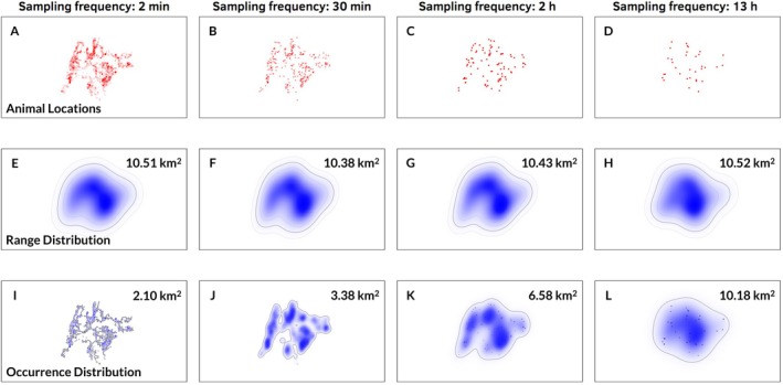 FIGURE 1
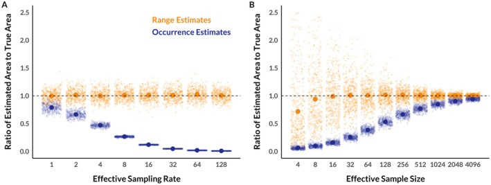 FIGURE 2
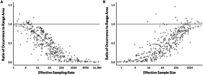 FIGURE 3
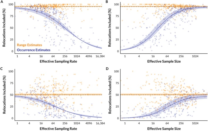 FIGURE 4
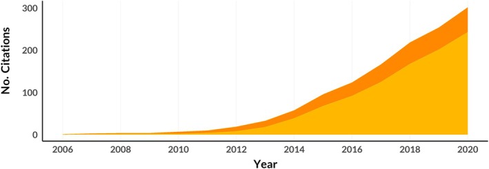 FIGURE 5
| Movement model | Position autocorrelation | Velocity autocorrelation | Range residency |
|---|---|---|---|
| IID | No | No | Yes |
| BM | Yes | No | No |
| OU | Yes | No | Yes |
| IOU | Yes | Yes | No |
| OUF | Yes | Yes | Yes |
| Range distribution | Occurrence distribution | |
|---|---|---|
| Distribution type | Marginal | Conditional |
| Finite coverage area | Arises only when the stochastic movement process being modeled has a finite coverage area | Arises when the sampling rate is finite, regardless of whether the stochastic movement process being modeled has a finite coverage area |
| Statistical operation | Extrapolation (Over what area is an animal likely to range in the future?) | Interpolation (At which locations might an animal have occurred in the past?) |
| Sampling dependence | No (If its statistical assumptions are met, an estimator of range distributions will estimate stable coverage areas even as a movement track is sampled more frequently) | Yes (If its statistical assumptions are met, an estimator of occurrence distributions will estimate smaller coverage areas as a movement track is sampled more frequently) |
| Appropriate questions & examples | How large is an animal's home range?1–3 How do environmental and social factors influence animal area requirements?4–6 Where are individual animals likely to interact over time?7 What area is available to an animal in studies of third‐order habitat selection?8–10 | How likely is it that an animal visited a location of interest?11–14 Where might an animal have crossed a linear feature?15–17 When and where could two individual animals have interacted?18 In which areas of a landscape did an animal visit high‐priority resources (e.g., migratory corridors, stopover sites, or feeding grounds)?19–21 |
- —Bundesministerium für Forschung, Technologie und Raumfahrt10.13039/501100002347
- —Natural Sciences and Engineering Research Council of Canada10.13039/501100000038
- —National Science Foundation10.13039/100000001
- —Deutsche Forschungsgemeinschaft10.13039/501100001659
- —Sächsisches Staatsministerium für Wissenschaft, Kultur und Tourismus
Peer Reviews
No public reviews on file for this paper yet. If you reviewed it on a platform where reviews are public (OpenReview, ICLR, NeurIPS, ICML), you can paste yours below so the community can read it here.
Videos
No videos yet. Explain this paper in a talk, walkthrough, or lecture? Add one.
Taxonomy
TopicsDiffusion and Search Dynamics · Species Distribution and Climate Change · Wildlife-Road Interactions and Conservation
INTRODUCTION
Understanding how and why animals use the areas they inhabit is a core goal in the fields of ecology and conservation biology (Jeltsch et al., 2013; Nathan et al., 2008; Schick et al., 2008; Sutherland et al., 2013). The attributes of the areas where animals live shape their fitness, and knowledge of relationships between movement and fitness can inform our understanding of how animals interact with each other and their environments, as well as our ability to implement effective conservation interventions (Allen & Singh, 2016). For these reasons, the importance of quantifying space use was recognized early in the development of ecology and led to the concepts of “home ranges” and “utilization distributions.” The conceptual definition of home ranges provided by Burt (1943) is still the most widely cited and targeted for estimation. Burt defined an animal's home range as “…that area traversed by the individual in its normal activities of food gathering, mating, and caring for young. Occasional sallies outside the area, perhaps exploratory in nature, should not be considered as part of the home range.” Two and a half decades after Burt offered this definition, Jennrich and Turner (1969) coined the term “utilization distribution” as the probabilistic representation of a home range, providing a foundation for translating Burt's conceptual idea into statistical estimators that can be applied to animal location data (Horne et al., 2020). Together, these ideas have served as the foundation of research on animal movement and resource use over the past half a century.
Movement and resource use, however, are multifaceted aspects of animal behavior. Consequently, the home range concept has broadened substantially over time and there now exists a very large literature describing different approaches to home range estimation (Fieberg & Börger, 2012; Heit et al., 2021; Horne et al., 2020; Kie et al., 2010). Many of these approaches cluster around two distinct spatial probability distributions that arise from stochastic movement processes and can be estimated from animal location data. Fleming, Fagan, et al. (2015), and Fleming et al. (2016) referred to these as “range” and “occurrence” distributions, and others have begun to adopt this terminology (Horne et al., 2020; Keith et al., 2019; Scharf et al., 2018; Schlägel et al., 2019; Signer & Fieberg, 2021). Specifically, range distributions—which are most commonly estimated using minimum convex polygons (Dalke & Sime, 1938) and (autocorrelated) kernel density estimation (Fleming, Fagan, et al., 2015; Worton, 1989)—describe the long‐run behavior of a movement process that features restricted space use and are consistent with Burt's classic definition of the home range. In contrast, occurrence distributions—which are most commonly estimated using (dynamic) Brownian bridge movement models ([d]BBMMs; Horne et al., 2007; Kranstauber et al., 2012)—quantify uncertainty in the movement path of an individual during a period of observation and are not directly related to Burt's definition of the home range. If considering a random point along the sampled movement path as a prediction target, the occurrence distribution and range distribution are analogous to confidence intervals and prediction intervals, respectively, though both distributions are based on predictions. Both distributions can serve as estimation targets for which specific statistical estimators can be derived, but estimators of range distributions quantify fundamentally different phenomena than estimators of occurrence distributions: estimators of range distributions answer the question: “How much space is an animal likely to use over the long term?,” while estimators of occurrence distributions answer the question: “Where did an animal travel during a defined period of observation?” Although these questions may appear similar, range and occurrence distributions have very different biological and mathematical interpretations.
In this paper, we argue that range and occurrence distributions can serve as focal points around which to organize concepts, models, statistical estimators, and research questions. We use theoretical arguments, simulations, and empirical examples to demonstrate similarities and differences between these distributions, as well as consequences that can arise from conflating them (most commonly by using BBMMs to estimate home ranges). We then link estimators of range and occurrence distributions to the ecological questions each can answer.
CONCEPTS AND DEFINITIONS
By explicitly separating the discrete‐time and often arbitrary sampling schedule from the underlying continuous‐time movement process, continuous‐time movement models offer a number of advantages over the more traditional approach of assuming a discrete‐time movement process (Kareiva & Shigesada, 1983; Langrock et al., 2012; Morales et al., 2004). These advantages include the ability to estimate scale‐invariant parameters, the ability to model movement using irregularly sampled data, and freedom from the assumption of serial independence among datapoints (Fleming et al., 2014b; Gurarie et al., 2017; Johnson et al., 2008). Defining movement in this way provides a framework that facilitates the derivation of rigorous statistical procedures for quantifying movement (Blackwell, 1997; Dunn & Gipson, 1977; Fleming, Fagan, et al., 2015; Hanks et al., 2015; Johnson et al., 2011; Michelot, Blackwell, & Matthiopoulos, 2019), including many non‐random behaviors such as migration, territoriality, patrolling, trap‐lining, collective movement, and habitat‐ or condition‐specific movement (e.g., Brennan et al., 2018; Moriarty et al., 2017; Papageorgiou & Farine, 2020; Péron et al., 2017; Sawyer et al., 2019). In this framework, we may consider an animal's trajectory collected from a telemetry movement track, with coordinates, rt=xtyt, to be a realization from a continuous‐time stochastic process, Rt, that is observed at discrete times t1,t2,t3,⋯,tn. From this realization, we can predict and estimate quantities related to the animal's movement patterns, conditional upon stochastic movement models that can be used to generate movement trajectories (Table 1). Some, but not all, stochastic movement models are range‐resident and feature finite coverage areas, in that their coverage areas—the smallest area in which a given percentage of an animal's locations is predicted to occur—converge to a finite extent as t approaches infinity (Table 1). This property manifests as an asymptote in semi‐variance function of a stochastic process as the time lag between observations of the process increases (Fleming et al., 2014a). Brownian motion (Einstein, 1905; Horne et al., 2007) and the integrated Ornstein–Uhlenbeck (IOU) process (Gurarie et al., 2017; Gurarie & Ovaskainen, 2011; Johnson et al., 2008) are endlessly diffusing processes and thus do not have finite coverage areas (i.e., their coverage areas expand forever). In contrast, models such as the Ornstein–Uhlenbeck (OU; Dunn & Gipson, 1977; Uhlenbeck & Ornstein, 1930) and Ornstein–Uhlenbeck foraging processes (OUF; Fleming et al., 2014a; Fleming, Subaşı, & Calabrese, 2015) are range‐resident and feature finite coverage areas. The OU and OUF processes can be thought of as range‐resident versions of Brownian motion and IOU processes, respectively. Another key distinction among movement models arises from the types of autocorrelation they can accommodate. Brownian motion and OU movement produce autocorrelated positions but uncorrelated velocities, while IOU and OUF movement produce both autocorrelated positions and autocorrelated velocities. In contrast, the independent and identically distributed (IID) process, while having a finite coverage area, produces—as the name implies—completely uncorrelated data. With these movement models in mind, we can define two key families of distributions that capture many (but not all) conceptions of “space use” in the ecological literature.
The range distribution
Movement processes that feature finite coverage areas, including the IID, OU, and OUF processes, allow the possibility of a marginal probability density function prt=pRtrt at each time t, which is the probability density of a location rt at time t for the stochastic process Rt, without conditioning on any previous or subsequent locations. In the most general sense, a range distribution is a marginal distribution focused on a particular time frame or suite of movement behaviors—possibly averaged over times or behavioral states—to enable predictions of an animal's locations in future periods. In other words, a range distribution describes the probability of an animal being in a location at a given time, taking into account all of the locations in a movement track simultaneously. The range distribution is simplest to define for stationary processes, which describe unchanging movement behaviors:
for any time t. Non‐stationary processes, which describe movement behaviors that change over time (e.g., migrations, drifting home ranges), may further require an appropriate time average to weight the relevant marginal distributions (e.g., Fleming et al., 2018, S1). Because prangestationaryr denotes the relative frequencies of different locations of an animal in space, the range distribution provides a prediction of space use, in that 95% of future locations will fall within its 95% coverage area, so long as the underlying movement process does not change (a testable assumption; see Noonan et al., 2019).
Range distributions therefore quantify the long‐run (asymptotic) behavior of a movement process. They are generated by running a single realization of the movement process forward into the future while keeping movement behavior fixed. The coverage areas of the range distribution are not estimates of what space the animal has used during the observation period, but predictions of what space will eventually be used, given a sufficient amount of time for the movement process to continue. All else being equal, an IID process will very quickly enable accurate estimation of a range distribution as the sample size is increased, whereas highly autocorrelated processes such as OUF will take longer to enable accurate estimation of a range distribution, because their effective sample sizes will be much smaller than their nominal sample sizes. However, the autocorrelation in the resulting data contains information about the long‐run behavior of the process, and thus the estimate of the range distribution that accounts for autocorrelation in the data may contain a considerable amount of space that is not visited during a period of study. The range distribution corresponds closely to Burt's conceptual definition of home range because it quantifies the area that the animal typically uses, not including exploratory forays. Estimators of range distributions are thus the appropriate tools for answering the question: “How large is an animal's home range?”
Range distributions are part of a larger class of distributions called “limiting distributions” that describe the long‐run behavior of a stationary stochastic process. Although the value of limiting distributions for conceptualizing and characterizing animal movement processes has not been widely appreciated among movement ecologists, there has been some recent methodological development around this idea. Barnett and Moorcroft (2008) described a limiting distribution for resource selection models that can be used to inform mechanistic home range analysis (Moorcroft et al., 2006). Whitehead and Jonsen (2013) and Wilson et al. (2018) described limiting distributions of discrete‐space continuous‐time Markov chain processes that produce range distributions. Michelot, Gloaguen, et al. (2019) used the limiting distribution of a Langevin diffusion process to create utilization distributions, and also used Markov chain Monte Carlo sampling to construct a movement model whose limiting distribution is a known utilization distribution (Michelot, Blackwell, & Matthiopoulos, 2019).
When data are statistically independent, and thus consistent with the IID assumption, the range distribution can be estimated using a variety of methods including minimum convex polygons (MCPs), conventional kernel density estimation (KDE), and mechanistic home range analysis. For the autocorrelated data provided by modern technologies such as GPS and ATLAS (Kays et al., 2015; Nathan et al., 2022), the range distribution is most accurately estimated by autocorrelated Gaussian density estimation (Dunn & Gipson, 1977; Fleming et al., 2014b) if the home range is Gaussian, or autocorrelated kernel density estimation (AKDE; Fleming, Fagan, et al., 2015, Noonan et al., 2019) if the home range is not Gaussian. In other words, the estimation target of all of these estimators is the range distribution, but each estimator differs in the assumptions made about the data that underlie it. A given estimator must therefore be used only when the data are consistent with the movement model that underlies that estimator's assumptions (as is standard statistical practice).
Finally, we note that there is no dependence in the definition of the range distribution on the particular sampling regime chosen by an investigator. The range distribution is a property of the movement process that is independent of the sampling process. However, estimators of the range distribution are subject to a number of biases, some of which can be related to the sampling process (Silva et al., 2022). First, uncertainty in the size and shape of an estimated range distribution decreases in proportion to its “effective sample size,” which is approximately the number of times a focal animal moved far enough to cross its home range during an observation period. If the animal has not yet moved far enough to cross its range in an observation period, it is not possible to estimate an accurate range distribution, and if an animal has not crossed its range very many times in an observation period, it is difficult to accurately or precisely estimate range distributions. Uncertainty in estimates of range distributions can be in part represented by confidence bands around estimated coverage areas, as the coverage areas are often the key parameters of interest. Second, different estimators of range distributions may exhibit either positive or negative biases that decrease asymptotically as sampling duration increases. Third, estimators that assume IID data (e.g., conventional KDE, MCP, mechanistic home range analysis) tend to underestimate the size of home ranges when applied to autocorrelated tracking data by an extent that depends, all else equal, on the strength of autocorrelation in the sampled locations (Noonan et al., 2019). Again, this is not an inherent property of the range distribution per se, but, instead, results from using estimators for which a core assumption has been violated. As with any statistical procedure, violating a key assumption of a home range estimator can produce biased results.
The occurrence distribution
Whereas range distributions are based on the marginal probability density functions, prt, and can predict future locations, occurrence distributions are based on the conditional probability densities prtdata and are focused on interpolating the specific movement path that an animal took during an observation period and that connected a series of sampled locations. Such conditional distributions exist for all stochastic movement processes, even when those processes do not have finite coverage areas in the long run and do not describe range‐resident movement behaviors (e.g., Brownian motion and IOU movement). The simplest occurrence distribution that we can construct involves uniformly averaging these conditional densities over the observation period for times sampled between t1 and tn:
which summarizes the full information on the unknown path contained in the time‐indexed conditional densities, prtdata, into a single probability density, poccurrencer. This corresponds to the prediction of an unknown location rt at a random time t within the observation window, given the observed data. Missing observations are often skipped to avoid oversmoothing (e.g., Bedrosian et al., 2018; Coe et al., 2015; Sawyer et al., 2009), but weighting or imputation schemes that maintain a balance between detail and continuity (e.g., Buderman et al., 2016; Hooten & Johnson, 2017; Scharf et al., 2017) are available. In the limit of very coarse, uncorrelated data, and with some gap‐skipping heuristic applied, the occurrence distribution reduces to the empirical distribution of the data. This means that there must be detectable autocorrelation in the movement process for estimators of occurrence distributions to produce informative predictions of movement between observed locations—estimating an occurrence distribution using data that are so coarse as to be IID, or nearly so, will provide little information on unobserved locations.
Occurrence distributions quantify where an animal may have traveled during a given period of time, conditional on observed locations sampled within that period, and rely on autocorrelated movement models to interpolate the data between observed locations. They are not well estimated by the range distribution estimators outlined in the prior subsection, and occurrence distribution estimators have not been around nearly as long as range distribution estimators—the first estimator of occurrence distributions was introduced in the peer‐reviewed ecology literature less than 20 years ago (Horne et al., 2007). Occurrence distributions are calculated via model‐based time‐series Kriging, and Fleming et al. (2016) presented the general case. Earlier approaches to estimating occurrence distributions in the literature assumed specific movement models, such as Brownian motion (Horne et al., 2007; Kranstauber et al., 2012) or integrated Ornstein–Uhlenbeck motion (Johnson et al., 2011). Occurrence distributions exist for any autocorrelated movement process, however, whether or not the focal process assumes range‐resident movement. This means that the Brownian motion, IOU, OU, and OUF continuous‐time processes all admit occurrence distributions. For an IID process, the occurrence distribution is simply the empirical distribution, given some heuristic to account for gaps in the data. If large gaps are not skipped, then the effectively unconditioned predictions within those gaps will be as widespread as the underlying range distribution (infinite for Brownian and IOU motion) and will oversmooth the occurrence distribution into a large normal distribution.
Importantly, an estimator of occurrence distributions does not predict a movement path itself (because the movement path is a random variable, it is predicted rather than estimated), but uncertainty around that movement path—the movement path itself is best predicted by Kriging the most likely path, and occurrence distributions are the time‐average of that Kriging process' uncertainty distributions (i.e., the average predictive uncertainty around the most likely path); (Fleming et al., 2016). Estimates of the coverage areas of occurrence distributions are generated by considering all possible trajectories that are consistent with the data, weighted by their probability density. As the movement path of an animal becomes more finely and more accurately resolved, these coverage areas become smaller and smaller, eventually limiting to zero, even though the actual space used has not changed. Estimated coverage areas of occurrence distributions therefore do not directly measure space use—even during the observation period—but are, instead, a reflection of our uncertainty regarding where an animal was located during an observation period. In other words, if we have complete knowledge of the animal's locations during an observation period (i.e., infinite sampling rate and no location error), estimates of the occurrence distribution collapse to the animal's movement path and have zero area. The occurrence distribution is thus appropriate for answering questions such as “Where might an animal have traveled during an observation period?” and “What landscape features might an animal have visited along its movement path?”
Transitioning from marginal distributions that are independent of specific observations to conditional distributions that are conditional upon preceding and subsequent observations has a dramatic effect on the meaning and operation of occurrence distributions. Range distributions and their constituent marginal distributions are parameters of the movement process that exist independently from the sampling process (though estimators of the range distribution may exhibit some sampling dependence). In contrast, occurrence distributions are conditional upon samples of data and are explicitly defined in terms of the sampling schedule. This means that a different sampling schedule applied to the same movement process will correctly yield a different occurrence distribution: all else equal, increasing the sampling rate will result in a narrower, more concentrated occurrence distribution. This happens because more frequent sampling more fully resolves the animal's true movement path, and thus uncertainty in the animal's locations decreases concomitantly. It is important to realize that this is not due to sampling‐dependent bias of estimators of occurrence distributions: occurrence estimators in the time‐series Kriging family, including the BBMM, can be unbiased. Instead, the uncertainty decreases because the estimation target itself (i.e., the occurrence distribution) is a function of the sampling schedule. Figure 1 shows this process occurring for data from a fisher (Pekania pennanti) tracked for 19 days in New York, USA, at a roughly 2‐min sampling interval.
Demonstration of sampling dependence of estimated occurrence and range distributions using location data from a GPS‐tracked fisher (Pekania pennanti) from New York, USA. The fisher was tracked for 19 days at 2‐min intervals. The top row (panels A–D) features individual locations along the fisher's movement track as the movement track is progressively thinned from ca. 720 locations per day to ca. 2 locations per day. The second row (panels E–H) features estimated 95% coverage areas generated using autocorrelated kernel density estimation on these GPS locations. While the contours of the estimated range distribution change as the data are more finely resolved, the size of estimated coverage areas (labeled in the upper right of each panel) remains largely stable. The third row (panels I–L) features estimated 95% coverage areas by Kriging the same GPS location. In contrast with the estimated coverage areas of the range distributions, the size of estimated coverage areas of the occurrence distributions (also labeled in the upper right of each panel) decreases rapidly as the data are sampled more frequently and uncertainty in the fisher's movement path decreases. With the coarsest samples (panels H and L), estimated coverage areas for the two methods are similar. With the finest samples (panels E and I), however, the estimated coverage area of the occurrence distribution is only ca. 20% of the size of the estimated coverage area of the range distribution.
While the occurrence distribution itself is a reflection of uncertainty in the unknown movement path, its parameter uncertainty has not been historically propagated. In fact, parameter uncertainty has only recently been propagated even among range distributions (Fleming & Calabrese, 2017), where the key parameters of interest are the coverage areas. However, for occurrence distributions, the key predictions of interest are expected values of spatial covariate functions. For instance, the expected value with respect to a vegetation cover index is the point prediction for the average of percent vegetation cover sampled along the unknown movement path (e.g., 70%). For these expected values, there is both the predictive uncertainty, reflecting the unknown movement path, and estimation uncertainty, reflecting the unknown movement parameters.
Relationships between range and occurrence distributions
As detailed above, range and occurrence distributions are based on different biological and statistical definitions, have different interpretations and statistical estimators, and respond differently to variation in sampling schedules. We now consider two key limits defined by data amount and quality that highlight the conditions under which range and occurrence distributions either converge or diverge completely, and reiterate a conceptual difference between the two distributions.
Convergent limit: Infinite observation period
Given an infinite observation period, the occurrence distribution will converge to the range distribution for range‐resident movement processes. This happens because an animal visits more and more of its home range over time. Differences in estimated range and occurrence distributions can still arise from estimation error caused by gaps in data and measurement error. Decreasing location error and increasing the sampling rate will reduce this estimation error, but increasing the sampling rate will also slow down convergence because coverage areas of occurrence distributions limit to zero if the sampling rate is infinite while the observation period is finite.
Divergent limit: Infinite sampling rate
For the occurrence distribution of any realistic movement process that is continuous in both location and velocity, holding the sampling duration constant while increasing the sampling rate with either no location error or uncorrelated location error yields the limit:
where δr is the Dirac delta function—a singular distribution with probability mass concentrated at r, and where rt is the realized location. In other words, as sampling becomes finer and finer, the occurrence distribution collapses to the movement path with zero coverage area, even in the presence of (uncorrelated) location error. This limit is easiest to see in the case of a BBMM, where the width of the bridge is at its most proportional to dt. The range distribution is not subject to this limit and estimates of its coverage areas remain the same, though estimators of the range distribution may exhibit varying dependence on sample size. Increasing the rate of sampling results in increasingly strong autocorrelation in the data, so estimators of range distributions that do not account for this autocorrelation perform worse as sampling rate increases, all else being equal. Such estimators are increasingly negatively biased by increasing autocorrelation strength and will also limit to zero area. However, estimators of range distributions that properly model autocorrelation will be unaffected by this limit, and estimated coverage areas will remain consistent.
Extrapolation versus interpolation
Range and occurrence distributions can also be conceptualized in terms of two common categories of statistical inference: extrapolation and interpolation, respectively. Given a sample of tracking data of finite duration, an estimate of the range distribution represents an extrapolation of the long‐run behavior of the movement process, as inferred from the data, and quantifies the variance of the movement process. In contrast, an estimate of the occurrence distribution interpolates within the observation period, conditional on the data and an autocorrelated movement model, and quantifies uncertainty in the interpolation. This is why the general framework for estimation of occurrence distributions is based on Kriging, which is a statistically optimal method of model‐based interpolation (Fleming et al., 2016).
To illustrate this more concretely, consider the differences in how cross‐validation of estimators of home range distributions and cross‐validation of estimators of occurrence distributions are performed. If an estimator accurately quantifies the areas of home ranges (sensu Burt, 1943), 95% coverage areas of home ranges generated over some observation periods T1 should contain, on average, 95% of those same animals' locations over subsequent observation period T2, provided those animals' movement behaviors do not meaningfully change between training (T1) and test (T2) sets, and provided that T1 and T2 begin far enough apart to be uncorrelated. If 95% coverage areas of home ranges consistently include more than 95% of the locations in test sets, then estimators are overestimating the sizes of home ranges; if those coverage areas consistently include fewer than 95% of locations in test sets, then estimators are underestimating the sizes of home ranges. Similarly, 50% coverage areas generated over T1 should contain 50% of animals' locations, on average, over T2. In other words, the relevant test set for an estimator of range distributions is a set of locations sampled from an animal's movements in the future, extrapolated from past locations (half‐sample cross‐validation; e.g., Noonan et al., 2019). Cross‐validation of estimators of occurrence distributions should operate differently. If an estimator quantifies occurrence distributions accurately, 95% coverage areas estimated using locations sampled from T1 should contain 95% of those animals' unobserved locations occurring within T1. In other words, the relevant test set for an estimator of occurrence distributions is holdout data from within an observation period (and not a subsequent period).
SIMULATED EXAMPLES
The two limits described above are crucial for understanding the differences between occurrence and range distributions. We now demonstrate the importance of these limits with both simulated and real data. For the simulated data, we can specifically model processes where both types of distributions exist: processes that are (1) autocorrelated (so that estimators of the occurrence distribution can interpolate the data) and (2) range‐resident (so that a range distribution exists). Simulation also allows us to set known parameters for the home range (range distribution). We can then manipulate the sampling schedule of the simulated processes to explore the effects of sampling rate and sampling duration on the sizes of estimated range and occurrence distributions. To do this, we simulated movement paths from an OUF process while varying the sampling rate and sampling duration systematically to illustrate differences between estimates provided by estimators of range and occurrence distributions. For each dataset, we estimated the range distribution via autocorrelated Gaussian density estimation conditioned on a fitted OUF model with daily autocorrelation timescales. Similarly, we estimated the occurrence distribution for each dataset by Kriging with an OUF model with daily autocorrelation timescales. The process that generated the simulated data exactly matches the statistical assumptions of these estimators, so any differences in size between estimates of the two distributions reflect differences in the distributions rather than differences in data used to estimate them.
Figure 2A shows the estimated coverage areas of the occurrence distribution decreasing in size as the sampling rate increases from one observation per day to 128 observations per day. Note that the estimated 95% coverage areas of the occurrence distribution start substantially smaller than the estimated 95% coverage areas of the range distribution, because the sampling duration is finite (256 days, in this case), and then rapidly collapses to zero as the sampling rate increases. Ongoing technological advances that facilitate ever finer and more accurate location sampling are driving movement studies closer to the limit where estimated occurrence distributions collapse to zero area. It is therefore inevitable that the differences between range and occurrence distributions will become more obvious in the future, even though these distributions have been frequently conflated in the past.
Bias in estimated home range size provided by coverage areas of range (orange) and occurrence (indigo) distributions estimated using data with different sampling rates (i.e., GPS fixes per range crossing; panel A) and effective sample sizes (i.e., number of range crossings in a dataset; panel B). A point at 1 indicates that home range size was estimated correctly for a simulated movement track with a known home range size. Small points represent a single simulation result (jittered on the x‐axis to ease visualization), while larger points represent the mean simulation result among 400 replicates. Divergence of estimated range distributions from the line at 1 at small durations of sampling arise from known patterns of bias that can be improved by bootstrapping (Fleming et al., 2019), while bootstrapping does little to change the size of estimated occurrence distributions.
Figure 2B shows the estimated coverage areas of the occurrence distribution increasing as the sampling duration increases from 4 to 4096 days. Again, the estimated 95% coverage areas of the occurrence distribution are still substantially smaller than the estimated 95% coverage areas of the range distribution even when the effective sample size (i.e., the number of range crossings) is >4000, and rapidly collapse to zero as the duration of the observation period decreases. This is a major real‐world problem because it can take weeks or months on average for an animal to cross its range (depending on species), and the lifespan of tracking devices (or even animals) is unlikely to enable an effective sample size of anywhere near 4000 (i.e., 11 years with daily range crossings). This demonstrates that while occurrence distributions tend toward range distributions as the sampling duration increases, using an estimator of occurrence distributions to quantify the size of home ranges will yield a substantial underestimate unless data are collected for a very long period of time—periods of time that are likely logistically and/or biologically impossible. Although technological advances are increasing the battery lifespan of animal tracking devices, and thus the potential duration of animal tracking studies, the duration of tracking data for an individual animal is often limited in practice by mortality or equipment failure. Estimators of occurrence distributions will therefore tend to provide estimated home ranges that are substantially smaller than the true size of home ranges in most real‐world situations.
EMPIRICAL EXAMPLES
Using empirical data, we now show how profoundly estimates of range and occurrence distributions can diverge in real‐world datasets. As outlined above, this happens when the data are sampled frequently enough that the occurrence distribution collapses toward the movement path and for long enough that estimating the range distribution is possible. Such datasets are already common and their availability will only increase as tracking technology improves (Gupte et al., 2022; Kays et al., 2015; Nathan et al., 2022). Using a dataset of 369 individual animals across 27 species (Noonan et al., 2019), we estimated both the range and occurrence distributions for each animal. We estimated the range distribution via autocorrelated kernel density estimation (AKDE) conditioned on a fitted movement model according to the workflow described in Silva et al. (2022). In short, we used variogram analysis (Fleming et al., 2014a) to ensure that animals were range‐resident, fit and selected an autocorrelated movement model that best described the animal's movements using perturbative hybrid residual maximum likelihood (phREML; Fleming et al., 2019) and Akaike's information criterion corrected for small sample sizes (AICc; Hurvich & Tsai, 1989), and estimated weighted AKDE utilization distributions for each animal (Fleming et al., 2018) using the ctmm R package (v0.6.2; Calabrese et al., 2016) in the R statistical software environment (v3.6.2; R Core Team, 2020). We estimated the occurrence distribution for each animal based on Kriging (Fleming et al., 2016) with the same movement model used for the corresponding AKDE estimate. Figure 3 shows that the estimated 95% coverage areas of occurrence distributions are smaller than estimated 95% coverage areas of range distributions for the vast majority of individuals in the dataset (and usually much smaller). This occurs because the effective sample size of real‐world datasets—which typically depends more on the duration of sampling than on the frequency of sampling—is rarely large enough to approach the theoretical limit where the occurrence distribution would converge with the range distribution.
The ratio of the size of estimated 95% coverage areas of occurrence distributions to the size of estimated 95% coverage areas of range distributions for a dataset containing 369 individuals across 27 species, as a function of the effective sampling rate (i.e., GPS fixes per range crossing; panel A) and effective sample size (i.e., number of range crossings in a dataset; panel B). Points represent individual animals, while dashed lines represent regressions demonstrating the overall trend. Solid horizontal lines indicate a ratio of 1:1, where estimated range and occurrence distributions are the same size. Distance below the solid line indicates the extent to which estimators of occurrence distributions are negatively biased in their estimates of home range size.
The smaller coverage areas of estimated occurrence distributions compared to estimated range distributions consistently lead to underestimation of the size of animal home ranges. To illustrate this, we performed half‐sample cross‐validation on the same animal location dataset. We subset data from each individual animal into halves, used the first half of the data to generate estimates of range distributions (via AKDE) and occurrence distributions (via Kriging), and then used the second half to assess the percentage of future animal locations that were within the estimated range and occurrence distributions. All data fit the assumptions of range‐resident animals with movement processes that remained consistent between the two halves. We then fit regression lines (linear for AKDE estimates, logistic for Kriged estimates) for the influence of effective sampling rate (roughly the number of GPS locations per range crossing) and effective sample size on the percentage of locations in the test set that fell within estimates generated using the training set.
As these results show (Figure 4), estimated home ranges produced by estimators of occurrence distributions do not merely fit the data more tightly—they inaccurately represent the size of home ranges. Estimated home ranges produced by estimators of occurrence distributions are nearly always too small, and this negative bias is exacerbated at high sampling rates and low effective sample sizes. This is not merely a hypothetical problem, nor is it only an issue that will arise in the future as technology continues to improve. Instead, it is pervasive in the animal movement data that wildlife biologists currently collect and analyze (Noonan et al., 2019; Noonan et al., 2020).
Half‐sample cross‐validation of estimated range and occurrence distributions. Points represent the percentage of locations from the second half of the data (test set) included in home ranges estimated using the first half of the data (training set). Orange points represent range (autocorrelated Kernel density estimation) estimates, while indigo points represent occurrence (Kriging) estimates. The dashed line represents the target 95% (top row) or 50% (bottom row) quantile, while the solid line represents a regression model fit to the cross‐validation results with shading to indicate the 95% confidence interval. The left column demonstrates the influence of effective sampling rate on cross‐validation results, while the right column demonstrates the influence of effective sample size on cross‐validation results. On average, estimated range distributions contain roughly the correct percentage of relocations, and this remains true across all effective sampling rates and effective sample sizes. Estimated occurrence distributions, however, tend to contain too few relocations, and this problem is exacerbated at high effective sampling rates and low effective sample sizes.
DISCUSSION
Ecologists often conflate estimators of occurrence distributions with estimators of range distributions, a much older and more familiar class of statistical tools. The first widely used estimators of occurrence distributions (Horne et al., 2007; Johnson et al., 2011) were landmark advances in movement ecology and enabled more statistically rigorous analyses of many research questions related to animal movement. Nevertheless, although they have been widely used in movement ecology, their novelty and unique statistical properties have still gone unrecognized all too often. As we have demonstrated, estimators of range and occurrence distributions have radically different properties and should therefore be used for different purposes (Table 2). Ecologists and conservation biologists should use estimators of range distributions to estimate home ranges, and estimators of occurrence distributions to answer other questions, such as the following: How likely is it that an animal visited a location of interest (Johnson et al., 2011; Noonan et al., 2018; Pagès et al., 2019; Scharf et al., 2017)? Where might an animal have crossed a linear feature (Find'o et al., 2018; Hooker et al., 2020; Zeller et al., 2018)? When and where could two individual animals have interacted (Schlägel et al., 2019)? Which areas of a landscape contain high‐priority resources (e.g., migratory corridors, stopover sites, and feeding grounds; Johnson et al., 2011, Sawyer et al., 2009, 2019)?
Estimation of animal home ranges is foremost among our concerns on the conflation of range and occurrence distributions—estimators of occurrence distributions consistently and substantially underestimate the size of home ranges under a broad array of real‐world conditions (Figures 3 and 4). In recent years, there has been a slow but steady drift in preference among wildlife biologists toward estimators that fit more tightly to animal location data (Figure 5; Crane et al., 2021, Laver & Kelly, 2008, Walter et al., 2015). We believe that this preference has largely been driven by the intuitive notion that areas within estimated home ranges where an animal does not travel during a study are not actually “used” (Cumming & Cornélis, 2012; Getz et al., 2007; Kie, 2013; Walter et al., 2015). This preference can be observed in the transition over time from home range estimates using minimum convex polygons to local convex hull (LoCoH; Getz et al., 2007, Getz & Wilmers, 2004) to time local convex hull (T‐LoCoH Lyons et al., 2013) methods, an emphasis on KDE bandwidth optimizers that fit tightly to location data (Cohen et al., 2018; Downs & Horner, 2008; Kie, 2013), and most recently, rapid growth in use of BBMMs to estimate home ranges (Figure 5). Cross‐validation frameworks that seek to backtest estimator performance (e.g., Getz & Wilmers, 2004; Kie, 2013; Silva et al., 2020; Walter et al., 2015), which are appropriate for assessing estimators of occurrence distributions but not estimators of range distributions, have also provided a false impression that range estimators that generate smaller home ranges perform better. While understandable, seeking home range estimates that fit tightly to an animal's past locations adheres neither to Burt's widely cited definition nor the mathematical properties underlying the range distribution. Researchers typically aim to capture the amount of space an animal needs to survive and reproduce in the long run, not simply the level of uncertainty in an animal's movement path during an observation period limited by study design, technology, or animal mortality. When comparing multiple estimators, smaller home range estimates are only better if coverage areas provide predictions of future animal locations that are at least as unbiased as the estimator that produces the larger estimate.
Number of peer‐reviewed journal articles from 2006 to 2020 that either used Brownian bridge movement models (BBMMs) to estimate the size of animal home ranges (light orange) or labeled BBMMs as a home range estimator (dark orange). Although the BBMM is an estimator of occurrence distributions and therefore poorly suited for estimating home ranges, the use of BBMMs to estimate home ranges is growing rapidly.
The most common estimator of occurrence distributions used to estimate home ranges is the BBMM (Horne et al., 2007), which has even been championed as a “third generation home range estimator” due to its ability to account for some autocorrelation in tracking data (Walter et al., 2015). Figure 5 shows the cumulative number of peer‐reviewed journal articles between 2007 (when the BBMM was introduced to ecologists) and 2020 that either label it a home range estimator or use it to estimate the sizes of animal home ranges. However, Fleming et al. (2016) formally proved that the BBMM is an estimator of the occurrence distribution (rather than the range distribution) that arises as a special case of the more general time‐series Kriging family of estimators of occurrence distributions. Specifically, Kriging a movement track conditional on a Brownian motion movement model is equivalent to the BBMM. Beyond being an estimator of occurrence distributions, and thus only suited to the task of home range estimation in the (unrealistic) infinite data limit, the BBMM is also based on an endlessly diffusing Brownian motion process, which does not have a finite coverage area. Note that this is not a critique of the validity of the BBMM as an analytical tool per se. Other estimators of occurrence distributions, such as time‐series Kriging conditional on an OUF movement process, are also inappropriate for estimating the sizes of home ranges (as demonstrated in Figures 1, 2, 3), and BBMMs are the best tool currently available for quantifying where an animal might have been during an observation period if the Brownian motion model accurately characterizes the animal's movement process. Furthermore, when BBMMs were developed, the issue of underestimation of home ranges as outlined above was not as apparent because animal location data were coarser than they are today. However, as animal tracking technology improves and the resolution of datasets increases, the discrepancy between the coverage areas that BBMMs estimate and proper coverage areas for range distributions will continue to widen, and repeated studies of the same species with improved technology will lead to progressively smaller estimates of home ranges if these estimates are generated using estimators of occurrence distributions like BBMMs.
Using estimators of occurrence distributions to quantify home ranges can therefore have pernicious consequences for area‐based conservation strategies and for ecological inference. For example, many protected areas (e.g., the Attwater Prairie Chicken National Wildlife Refuge, Kirtland's Warbler Wildlife Management Area, and the National Key Deer Refuge in the USA, the Arawale National Reserve in Kenya, and the Blackbuck Conservation Area in Nepal) are designed to protect a focal species. For these protected areas, understanding how much space is required to maintain populations that are viable over the long term is vital for ensuring their effectiveness (Brashares et al., 2001; Pe'er et al., 2014). When protected areas are too small relative to their focal species' area requirements, the probability of population declines or extirpation increases significantly (Brashares et al., 2001; Gaston et al., 2008). Undersized protected areas also force a greater proportion of individuals into human–wildlife conflict at protected area boundaries (van Eeden et al., 2018) as relatively more animals must forage outside of protected areas (Farhadinia et al., 2018). It is thus critical that policy actions be well informed on area requirements of target species. To ensure that protected areas are adequately sized, estimates of the area required for an individual of a given species to persist and reproduce are often quantified via home range analysis (Martins et al., 2013; Rechetelo et al., 2016; Tédonzong et al., 2018). Because estimators of occurrence distributions underestimate the future area traversed by GPS‐tracked animals (often dramatically so; Figure 4), using estimators of occurrence distributions to estimate area requirements can result in protected areas that do not accomplish their intended purpose.
Conflating range and occurrence distributions when quantifying space use is also dangerous in its implications for basic inference in ecology. For example, the distinction between range and occurrence distributions is particularly salient for studies of resource use and selection by animals. Resource selection is generally studied using resource selection functions—which compare environmental covariates at the locations where animals were present (i.e., “used” locations) to covariates at locations taken from an area assumed to be available for selection (i.e., “available” locations; Manly et al., 2007)—or resource utilization functions, which compare intensity of use among an animal's used locations (Marzluff et al., 2004; Millspaugh et al., 2006). Estimators of range distributions are appropriate tools for quantifying availability for resource selection functions, because they characterize the area an animal is likely to travel over the long term. In contrast, estimators of occurrence distributions are appropriate for quantifying resource use in resource utilization functions, because they characterize an animal's likely presence on the landscape during a study period. In practice, ecologists typically (and correctly) use estimators of range distributions to sample availability in resource selection functions, but often use estimators of range distributions rather than occurrence distributions to quantify habitat use in resource utilization functions (e.g., Berry et al., 2019; Johnston et al., 2020; Koizumi & Derocher, 2019; Prince et al., 2016; Winder et al., 2017; but see Eckrich et al., 2020; Marques et al., 2020; Petroelje et al., 2021). This may be because the initial papers on resource utilization functions (Marzluff et al., 2004; Millspaugh et al., 2006) used estimators of range distributions to generate utilization distributions (understandable because estimators of range distributions were the only tools available at the time—estimators of occurrence distributions had not been popularized yet). Nevertheless, an increasing number of methods for estimating occurrence distributions have become available over the past two decades (Fleming et al., 2016; Horne et al., 2007; Johnson et al., 2011), and we encourage ecologists to use these estimators of occurrence distributions—rather than range distributions—to quantify resource use in resource utilization functions.
Tracking data can and should be a resource for informing our understanding of animal ecology. Although we are now better positioned than ever to use tracking data to estimate different aspects of space use by animals, capturing maximal value from tracking data requires ecologists to understand and use the most rigorous statistical tools and definitions currently available. In this paper, we have highlighted the distinction between range and occurrence distributions, delineated the conditions under which they will behave similarly and differently, mapped ecological questions and statistical estimators to each distribution, and demonstrated the negative consequences of continuing to conflate these two distributions. Estimators of both range and occurrence distributions are readily available today in free and open source software (Calabrese et al., 2016; Calenge, 2006; Johnson et al., 2008; Nielson et al., 2013; Signer et al., 2019), and we encourage readers to explore the important distinction between range and occurrence distributions themselves.
AUTHOR CONTRIBUTIONS
Justin M. Calabrese conceived the idea; Christen H. Fleming developed the mathematical theory and arguments; Jesse M. Alston, Justin M. Calabrese, Christen H. Fleming, Michael J. Noonan, and Inês Silva conducted the analyses; and Jesse M. Alston and Justin M. Calabrese led the writing of the manuscript. Thomas S. B. Akre, Abdullahi H. Ali, Jerrold L. Belant, Dean Beyer, Niels Blaum, Katrin Böhning‐Gaese, Rogério Cunha de Paula, Jasja Dekker, Jonathan Drescher‐Lehman, Nina Farwig, Christen H. Fleming, Adam T. Ford, René Janssen, Florian Jeltsch, Peter M. Kappeler, Scott D. LaPoint, A. Catherine Markham, E. Patricia Medici, Ronaldo Gonçalves Morato, Ran Nathan, Kirk A. Olson, Bruce D. Patterson, Tyler R. Petroelje, Emiliano Esterci Ramalho, Sascha Rösner, Luiz Gustavo Rodrigues Oliveira‐Santos, Dana G. Schabo, Nuria Selva, Agnieszka Sergie, Orr Spiegel, Wiebke Ullmann, Filip Zięba, and Tomasz Zwijacz‐Kozica contributed data for empirical analyses. All authors contributed critically to drafts of the manuscript and gave final approval for publication.
CONFLICT OF INTEREST STATEMENT
The authors declare no conflicts of interest.
Supporting information
Appendix S1.
The reference list from the paper itself. Each links out to its DOI / PubMed record.
- 1Allen, A. M. , and N. J. Singh . 2016. “Linking Movement Ecology with Wildlife Management and Conservation.” Frontiers in Ecology and Evolution 3: 155.
- 2Alston, J. 2025. “Code and Metadata for: Clarifying Space use Concepts in Ecology: Range vs. Occurrence Distributions.” Dataset. Zenodo. 10.5281/zenodo.17676444.PMC 1296695441793168 · doi ↗ · pubmed ↗
- 3Barnett, A. H. , and P. R. Moorcroft . 2008. “Analytic Steady‐State Space Use Patterns and Rapid Computations in Mechanistic Home Range Analysis.” Journal of Mathematical Biology 57: 139–159.18064464 10.1007/s 00285-007-0149-8 · doi ↗ · pubmed ↗
- 4Bedrosian, B. E. , R. Domenech , A. Shreading , M. M. Hayes , T. L. Booms , and C. R. Barger . 2018. “Migration Corridors of Adult Golden Eagles Originating in Northwestern North America.” P Lo S One 13: e 0205204.30462652 10.1371/journal.pone.0205204 PMC 6248900 · doi ↗ · pubmed ↗
- 5Berry, L. E. , F. A. L'Hotellier , A. Carter , L. Kemp , R. P. Kavanagh , and D. A. Roshier . 2019. “Patterns of Habitat Use by Three Threatened Mammals 10 Years after Reintroduction into a Fenced Reserve Free of Introduced Predators.” Biological Conservation 230: 1–9.
- 6Bista, D. , G. S. Baxter , N. J. Hudson , and P. J. Murray . 2023. “Seasonal Resource Selection of an Arboreal Habitat Specialist in a Human‐Dominated Landscape: A Case Study Using Red Panda.” Current Zoology 69: 1–11.36974152 10.1093/cz/zoac 014PMC 10039176 · doi ↗ · pubmed ↗
- 7Blackwell, P. G. 1997. “Random Diffusion Models for Animal Movement.” Ecological Modelling 100: 87–102.
- 8Brashares, J. S. , P. Arcese , and M. K. Sam . 2001. “Human Demography and Reserve Size Predict Wildlife Extinction in West Africa.” Proceedings of the Royal Society B: Biological Sciences 268: 2473–2478.10.1098/rspb.2001.1815 PMC 108890211747566 · doi ↗ · pubmed ↗