The functional gait deviation index
Sajal Kaur Minhas, Morgan Sangeux, Julia Polak, Michelle Carey

TL;DR
Researchers developed a new index to measure gait abnormalities by considering smoothness and joint interactions, which can be used to assess walking disorders more effectively.
Contribution
The FGDI introduces a novel method that accounts for smoothness and co-variation in gait analysis.
Findings
FGDI scales with overall gait function and provides a consistent measure of gait abnormality.
FGDI is implemented as an interactive web app for easy use.
FGDI improves upon existing benchmarks by incorporating joint/plane smoothness and co-variation.
Abstract
A typical gait analysis requires the examination of the motion of nine joint angles on the left-hand side and six joint angles on the right-hand side across multiple subjects. Due to the quantity and complexity of the data, it is useful to calculate the amount by which a subject’s gait deviates from an average normal profile and to represent this deviation as a single number. Such a measure can quantify the overall severity of a condition affecting walking, monitor progress, or evaluate the outcome of an intervention prescribed to improve the gait pattern. The gait deviation index, gait profile score, and the overall abnormality measure are standard benchmarks for quantifying gait abnormality. However, these indices do not account for the intrinsic smoothness of the gait movement at each joint/plane and the potential co-variation between the joints/planes. Utilizing a multivariate…
Genes, proteins, chemicals, diseases, species, mutations and cell lines named across the full text — each resolved to its canonical identifier and authoritative record.
Click any figure to enlarge with its caption.
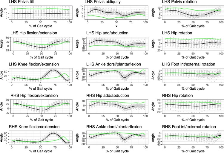 Figure 1
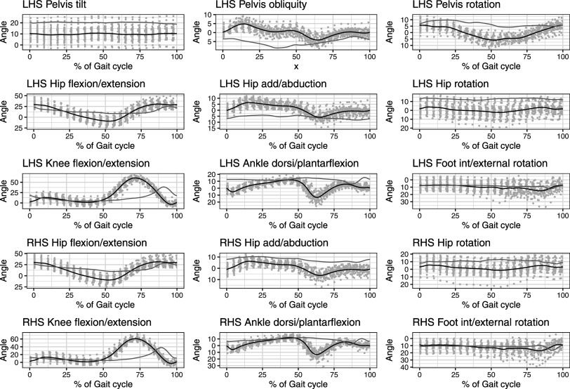 Figure 2
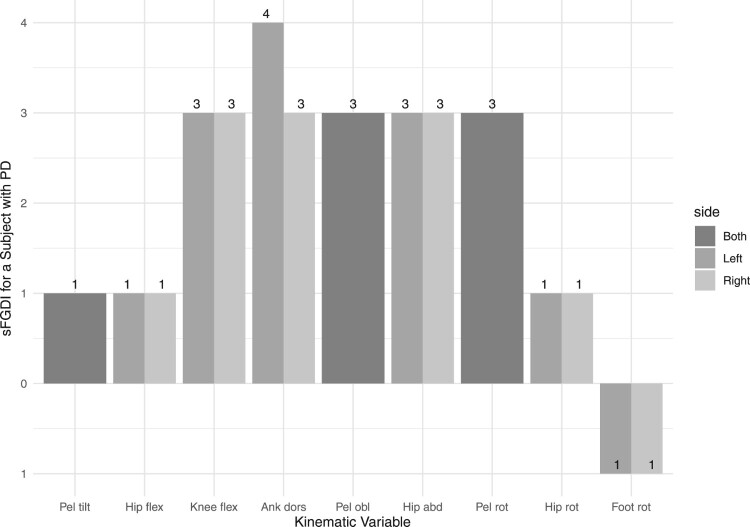 Figure 3
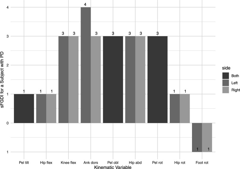 Figure 4
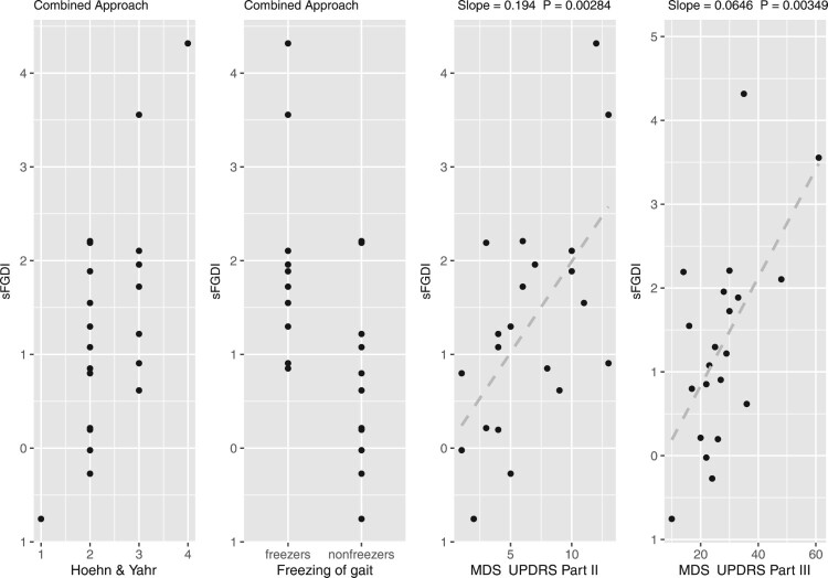 Figure 5
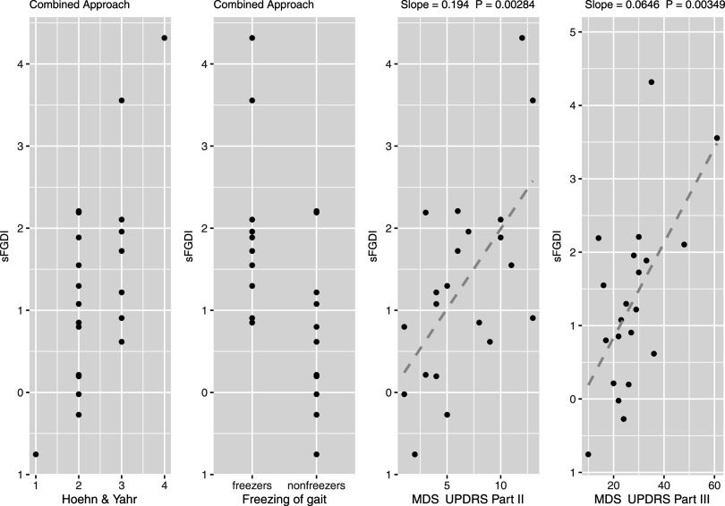 Figure 6
 Figure 7
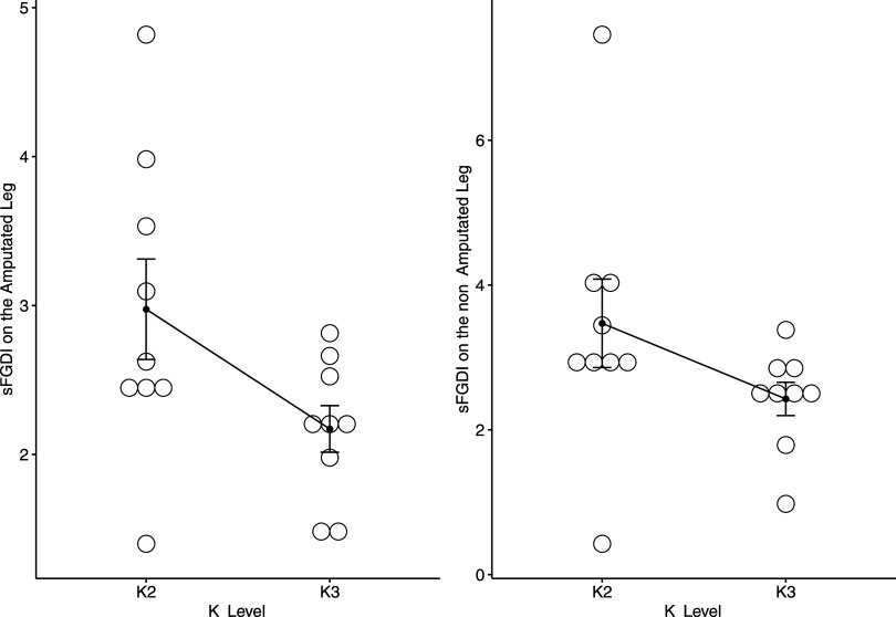 Figure 8
 Figure 9
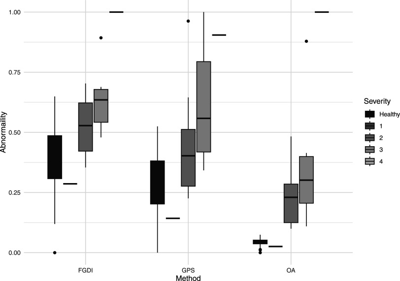 Figure 10
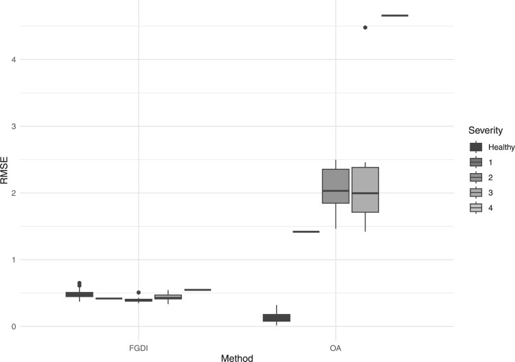 Figure 11
 Figure 12
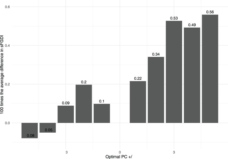 Figure 13
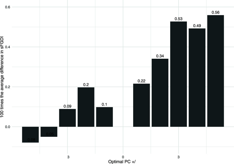 Figure 14
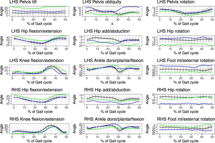 Figure 15
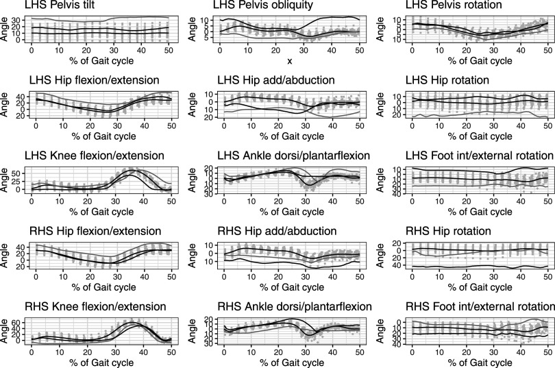 Figure 16
 Figure 17
 Figure 18
 Figure 19
 Figure 20
 Figure 21
 Figure 22
 Figure 23
 Figure 24
 Figure 25
 Figure 26
 Figure 27
 Figure 28
 Figure 29
 Figure 30
 Figure 31
 Figure 32
 Figure 33
 Figure 34
 Figure 35
 Figure 36
 Figure 37
 Figure 38
 Figure 39
 Figure 40
 Figure 41
 Figure 42
 Figure 43
 Figure 44
 Figure 45
 Figure 46
 Figure 47
 Figure 48
 Figure 49
 Figure 50
- —Science Foundation Ireland10.13039/501100001602
Peer Reviews
No public reviews on file for this paper yet. If you reviewed it on a platform where reviews are public (OpenReview, ICLR, NeurIPS, ICML), you can paste yours below so the community can read it here.
Videos
No videos yet. Explain this paper in a talk, walkthrough, or lecture? Add one.
Taxonomy
TopicsBalance, Gait, and Falls Prevention · Gait Recognition and Analysis · Diabetic Foot Ulcer Assessment and Management
Introduction
Typical gait data capture the movement of key kinematic variables throughout an individual’s stride. These variables encompass pelvic and hip angles across all three planes, knee flexion/extension, ankle dorsiflexion/plantarflexion, and foot internal/external rotation. Measurements are taken at 1% intervals throughout the entire 100% gait cycle. A prevalent objective in this analysis is to determine the extent to which an individual’s gait pattern deviates from the average gait pattern observed in a group of healthy subjects.
Figure 1 presents an illustrative example, displaying the gait patterns of 42 healthy subjects (depicted in grey) and their mean (shown in black), alongside the gait pattern of a subject with Parkinson’s disease (highlighted in green). This figure includes nine joint angles on the left-hand side and six on the right-hand side1. It is important to note that since the pelvis is common to both sides, it is appropriate to include pelvic kinematics from only one side.
As illustrated in Figure 1, the gait data are highly interdependent, with many kinematic variables exhibiting similar behavior across the gait cycle, planes, and joints. However, subjects with conditions affecting their walking patterns show significant differences, primarily due to variations in the timing and amplitude of their gait waveforms. Given the substantial amount and complexity of the data, there is a preference for employing a single metric to assess the extent of deviation in an individual’s walking pattern from the average pattern observed in a control group. This metric can be useful for assessing the overall severity of a walking impairment, tracking improvements over time, or evaluating the effectiveness of interventions aimed at enhancing walking patterns. Figure 1.The gait patterns of 42 healthy subjects (represented in grey) and their mean (shown in black), alongside the gait pattern of a subject with Parkinson’s disease (highlighted in green).
The Gait Deviation Index (GDI) and the Gait Profile Score (GPS) are established indices for assessing gait abnormalities, as detailed in Schwartz (2008) and Baker (2009), respectively. The GDI employs singular value decomposition on kinematic data from a reference database that includes all children who received gait analysis at the Gillette Children’s Specialty Healthcare Center between February 1994 and April 2007. This decomposition generates fifteen independent gait features that form the basis for projecting the kinematic variables of the subjects within any independently collected gait data sample. The GDI is calculated by measuring the distance between a subject’s projected kinematics and the average projected kinematics of the control group. GDI provides a metric for ranking individuals based on their deviation from the average behavior of the control group, offering distinct severity measures for the left and right legs.
The GPS is derived directly from the collected gait data sample as the root mean square difference between a subjects’s kinematic data and the average kinematic data of a control group. This measure provides an evaluation of gait abnormalities for both legs combined, each leg separately, and at the individual joint level. Such a detailed breakdown enhances understanding of which specific legs or joints contribute to gait abnormalities, thereby facilitating more targeted and effective treatment planning.
Although the GDI and GPS have been effective in assessing common gait pathologies such as cerebral palsy [17,21], rheumatoid arthritis [5], and Parkinson’s disease [8], they present inherent challenges. Kinematic variables for any individual are often highly correlated; the motion of one joint can significantly influence the motion of adjacent joints. Furthermore, the position of a joint at one point in the gait cycle strongly influences its position in later instances. This interdependence of kinematic data may result in biased assessments of overall abnormality when using the GDI and GPS indices, as demonstrated in [16].
The Overall Abnormality (OA) approach, introduced by Marks et al. [16], addresses the limitations inherent in the GDI and GPS. In contrast to the GDI, which derives its gait features from a historical reference database, the OA method applies principal component analysis (PCA) to kinematic data collected for the study’s control group, thereby deriving K independent gait features. A subject’s kinematic variables are then projected into this feature space, and the OA metric calculates the distance between the subject’s projected kinematics and the average of the projected kinematics for the control group. This method assesses severity across both legs, individually for each leg, and at each joint. However, utilizing PCA solely on the control group may lead to biased abnormality estimates, as the control group’s gait features might not adequately represent the patterns observed in subjects with significantly abnormal gaits. Moreover, while PCA recognizes the high interdependence of kinematic data, it does not fully address the essential structure of this dependence. The temporal sequence of kinematic data throughout the gait cycle is crucial in gait analysis and should be preserved. The interconnectedness across joints and planes often leads to multicollinearity, which can introduce bias in the measurement of overall abnormality.
In gait analysis, measurements are denoted by , where j ranges from 1 to 18, covering the pelvis and hip angles across all three planes, knee flexion/extension, ankle dorsiflexion/plantarflexion, and foot internal/external rotation for both the left and right sides. The index i represents individual subjects, numbered from 1 to N, and l indicates the observed points throughout the gait cycle, from 1 to T. To encapsulate the temporal ordering and the continuous nature of movement, a commonly employed approach [4,12,23,25] treats the set of discrete measurements as noisy realizations of a unified entity, a curve , representing the movement across the entire gait cycle t for each individual i and kinematic variable j. By aggregating these curves, we obtain a multivariate functional data set, so that for each individual a set of 18 functions is observed representing the movement for each of the 18 kinematic variables.
Multivariate Functional Principal Components Analysis (MFPCA) identifies the principal modes of variation within the covariance structure of the multivariate functional data set, accounting for potential covariations among the multiple kinematic variables. These modes represented as eigenfunctions of the covariance operator, capture significant deviations from the mean behavior of each kinematic variable. The principal component scores derived from these eigenfunctions provide insights into individual deviations from typical behavior. MFPCA effectively addresses potential multicollinearity issues due to interdependencies between joints or planes while preserving the temporal ordering throughout the gait cycle.
Applying MFPCA to the functional dataset yields independent gait features, into which any subject’s kinematic variables can be projected. Similar to the GDI and OA approaches, the proposed FGDI is calculated by measuring the distance between a subject’s projected kinematics and the average of the projected kinematics of the control group. Recently, Roach et al. [24] and Yoshida et al. [29] performed MFPCA on kinematic data and examined the resulting functional principal component scores to gain insight into the differences between two cohorts of individuals. These approaches differ from the proposed approach as they do not provide a single measure that can be used to quantify the overall severity of a condition or a means to rank the subjects based on gait pathology.
FGDI combines the advantages of the existing GDI, GPS and OA approaches. As the FGDI index is easy to interpret and can provide a measure of severity on both legs, as well as on each leg and at each joint separately. Additionally, the proposed approach accounts for the structure of the dependence of human gait leading to a more accurate quantification of gait pathology which can improve clinical decision-making.
Quantifying gait abnormalities
As discussed in the introduction, the conventional metrics used to quantify gait abnormalities include the GDI [26], the GPS [2], and the OA approach [16]. For more details on these approaches, please consult Sections A.1, A.2, and A.3 in Appendix 1.
In this section, we will begin by demonstrating how to apply the MFPCA technique, as described in [11], within the context of gait data. MFPCA is employed to identify the dominant modes of variation among individuals functions representing gait at each joint and within each plane. Subsequently, we will discuss the utilization of results from the MFPCA to compute the FGDI.
In gait analysis, data collection typically involves the recording of all 18 kinematic variables. However, subsequent analyzes focus only on specific subsets of these variables, tailored to the particular objectives of the study. For the computation of the FGDI, we concentrate on three distinct subsets of these variables, which are outlined as follows:
- Combined Approach: The first method involves using the combined observations from nine kinematic variables for the left side and six kinematic variables for the right side. Given that the pelvis is common to both sides, we include pelvic kinematics from one side only. This procedure results in the selection of fifteen kinematic variables, designated as . This approach yields a measure of severity by collectively considering both legs, thereby providing an overall assessment of gait abnormality.
- Individual Leg Approach: The FGDI can be calculated separately for each leg by utilizing the observations from the nine kinematic variables specific to that leg, designated with indices . This method provides a measure of gait pathology for each leg individually, facilitating a detailed assessment of gait abnormality in each leg.
- Joint/Plane Specific Approach: The FGDI can be computed for each kinematic variable separately, resulting in a measure of severity for each joint or plane, denoted by . This method offers a detailed evaluation of gait abnormalities at the individual level of each joint or plane.
Let the specific subset of kinematic variables be denoted by , where U represents either 15, 9, or 1, as described above.
Multivariate functional principal component analysis
2.1.
For each subject i, and kinematic variable u, the movement throughout the entire gait cycle can be expressed as follows:
where denotes the curve describing the movement of the uth kinematic variable for subject i evaluated at point within the gait cycle. The term represents the measurement error, which is presumed to follow a normal distribution with a mean of zero and constant variance . The function represents the inherent smoothness of gait movement throughout the entire gait cycle t. Let represent the centered gait data for the ith subject and the uth kinematic variable, observed at the T points over the gait cycle . Here, denotes the mean of across all subjects for the uth kinematic variable. The algorithm for obtaining the multivariate functional principal components, as outlined in [11], then proceeds with the following two steps:
- Calculate a univariate functional PCA on for each kinematic variable u. Here we use the functional PCA with fast covariance estimation attributable to [28]. This results in principal component functions and principal component scores, for each subject and each kinematic variable . The truncation lag for each variable, is chosen as the number of components that have a proportion of variance explained greater than ω, where ω is typically 0.99. When implementing the Joint/Plane Specific Approach, proceeding to step two is not necessary, as this method involves considering only a single joint or plane.
- Find the dominant modes of variation across multiple joints/planes: Combine all the principal component scores from each joint/plane into one big matrix with having rows and estimate the joint covariance matrix Perform a matrix eigen-analysis on to determine the eigenvectors and eigenvalues of for for some truncation lag . Here the truncation lag W is selected by the number of components that have a proportion of variance explained greater than ω, where ω is typically 0.99. The estimated multivariate orthonormal principal component scores are then given by:
for The MFPCA takes the co-variation between the different joints/planes into account by weighting the univariate functional principal component scores by the eigenvector of the covariance of the scores, representing the dependence across joints/planes, see [11] for further details.
The functional gait deviation index
2.2.
Denote the matrix of estimated principal component scores by . If we are interested in calculating an index representing the gait abnormality at each joint/plane (the joint/plane specific approach) then we use the univariate principal component scores in Step 1 in Section 2.1. That is for which implies . If we are interested in calculating an index representing the gait abnormality across multiple joints/planes accounting for the co-variation between the joints/planes (i.e. the individual leg or combined approach) then we use the multivariate principal component scores in Step 2 of the algorithm provided in Section 2.1. That is for which implies P = W.
First, calculate the average of the principal component scores from all healthy subjects, for . Then calculate the squared distance from the principal component score for the subject, , to the average principal component scores of all healthy subjects, which we denote by For details concerning the distribution of , please refer to Appendix 2. The FGDI for subject i is then given by the logarithm of the square root of the sum of the distances
The FGDI can be used in its raw format as a measure of gait pathology. Akin to GDI, to improve interpretation, we can scale the . Compute the sample mean and standard deviation of the FGDI for the healthy subjects denoted by and respectively. Then determine the z-score with respect to the healthy subjects
The scaled FGDI, in (2) can be interpreted as:
- Higher values of signify greater gait pathology.
- An value around 0 suggests a gait similar to that of an average healthy individual, indicating minimal or no gait pathology.
- Each unit deviation from 0 in the score represents an additional standard deviation from the average FGDI of healthy subjects. A positive deviation implies that the subject’s gait abnormality surpasses the typical level found in healthy individuals. Conversely, a negative deviation suggests that the subject’s gait does not exhibit abnormalities exceeding those typically observed in healthy individuals.
Assessing the severity of gait impairment in Parkinson’s disease patients
Parkinson’s disease (PD) is a widely prevalent, progressive neurodegenerative disorder characterized by substantial motor control impairments, including bradykinesia, tremors, rigidity, and gait instability. Global estimates in 2019 indicated that over 8.5 million individuals are affected by PD, representing a doubling of prevalence over the past 25 years [22]. Gait analysis is routinely utilized in clinical practice for severity stratification, treatment evaluation, and management of the condition.
The PD dataset is publicly accessible, as detailed in [27]. It includes data from 21 right-handed idiopathic PD individuals (5 females and 16 males), characterized by the following demographics: average age of 65 ± 10 years, average height of 166.5 ± 7.1 cm, and average mass of 71.89 ± 12.37 kg. Additionally, a healthy control dataset is available from [6], comprising 42 adults (18 females and 24 males). All participants were free from orthopedic or neurological diseases that could affect their gait. Their demographics are an average age of 43 ± 19 years, height of 167.1 ± 11 cm, and mass of 67.7 ± 11.2 kg.
The Hoehn and Yahr scale [13] is an established method for assessing the progression of PD, integrating medical evaluations with reports from patients and caregivers. The scale comprises four stages: Scale 1 is characterized by unilateral symptoms with minimal impact; Scale 2 involves bilateral symptoms without balance impairments; Scale 3 denotes moderate bilateral symptoms with some postural instability, though independence is retained; Scale 4 indicates severe disability, yet the ability to walk or stand is preserved. In the PD dataset, the distribution includes one subject at Scale 1, twelve at Scale 2, seven at Scale 3, and one at Scale 4.
The Movement Disorder Society’s Unified Parkinson’s Disease Rating Scale (MDS-UPDRS) [9] offers an alternative assessment for Parkinson’s Disease. This scale includes Part II, which evaluates motor experiences during daily activities, and Part III, which assesses motor functions including rigidity and agility. Higher scores on this scale reflect greater impairment. In the PD dataset, MDS-UPDRS Part II ranges from 1 to 13, and Part III ranges from 10 to 61.
Freezing of gait represents a notable motor symptom in PD, characterized by brief, episodic interruptions or significant reductions in the forward progression of the feet despite the intention to walk. This symptom can lead to falls and diminished independence. The dataset comprises ten patients experiencing freezing of gait (referred to as freezers) and eleven who do not exhibit this symptom (referred to as non-freezers).
For each subject, measurements of nine kinematic variables were recorded on both the left and right sides. These variables include pelvic tilt, pelvic obliquity, pelvic rotation, hip flexion/extension, hip abduction/adduction, hip rotation, knee flexion/extension, ankle dorsiflexion/plantarflexion, and foot internal/external rotation. The measurements consist of 101 equally-spaced time points throughout a single gait cycle, allowing the motion of each kinematic variable to be described in 1% increments of the gait cycle.
FGDI: the joint/plane specific approach
3.1.
The FGDI index is calculated using univariate principal component scores as described in Subsection 2.2 with the percentage of variation explained by the univariate principal components set to . This index quantifies the relative abnormality of a subject’s gait across each kinematic variable. The Movement Analysis Profile (MAP) displays the in (2) for the ith subject and uth kinematic variable. The height of each bar in the MAP represents the number of standard deviations by which the subject’s deviates from the average FGDI of healthy subjects. For illustrative purposes, Figure 2 depicts the MAP for a subject with PD, corresponding to the kinematic data presented in Figure 1. Figure 2.The MAP for a subject with Parkinson’s disease.
Figure 2 illustrates that the subject’s left-hand side ankle dorsiflexion/plantarflexion exhibits a significant deviation, measuring 4 standard deviations from the average FGDI of individuals without gait abnormalities. Conversely, the subject’s foot internal/external rotation aligns closely with standard gait patterns, as indicated by an FGDI value that is one standard deviation below the average for individuals without gait abnormalities.
It is well-established that unilateral motor symptoms are characteristic of PD, as underscored by Miller-Patterson et al. [20], Djaldetti et al. [3]. Correspondingly, most joints display comparable FGDI scores on both the left-hand side and right-hand side, except for notable discrepancies in ankle dorsiflexion/plantarflexion. This asymmetry in ankle gait patterns is consistent with recent research findings presented in [1].
Furthermore, the kinematic data presented in Figure 1 corroborates the values of the MAP, with higher values indicating trajectories, highlighted in green, that exhibit greater discrepancies from the mean of healthy individuals, shown in black. Conversely, lower values correspond to smaller discrepancies.
Table A1 in Appendix 4 demonstrates the optimal number of principal components required to account for 99% of the variance in the kinematic data, as well as 100 times the average difference in the FGDI across individuals when varying the number of principal components by plus or minus two. This analysis reveals that the FGDI remains highly stable, exhibiting minimal variations in FGDI values relative to the number of principal components.
FGDI: the combined leg approach
3.2.
We conducted an MFPCA on both legs, extracting 50 multivariate functional principal components. These components account for 99% of the variance in the kinematic data. Following this, we calculated the scaled FGDI in (2) using the MFPCA scores as described in Subsection 2.2.
Figure 3 presents the scaled FGDI values for all PD subjects in the sample. These values are categorized according to the subjects’ Hoehn and Yahr scale classifications, their designation as either freezers or non-freezers and their scores on the MDS-UPDRS Parts II and III. Figure 3.The scaled FGDI values for all PD subjects in the sample, grouped according to their Hoehn and Yahr scale, their status as either freezers or non-freezers and their scores on the MDS-UPDRS Parts II and III.
The subject exhibiting the highest scaled FGDI corresponds to the highest level on the Hoehn and Yahr scale, while the subject with the lowest scaled FGDI matches the scale’s lowest level. A Kruskal-Wallis rank sum test was conducted to evaluate whether median differences in scaled FGDI values are statistically significant relative to the Hoehn and Yahr scale, resulting in a p-value of 0.08. Subjects identified as freezers demonstrate higher scaled FGDI values compared to non-freezers, as confirmed by a Wilcoxon rank sum test with a continuity correction, which yielded a p-value of 0.007. Additionally, scaled FGDI values exhibit a linear increase with respect to the scores on Parts II and III of MDS-UPDRS, with slopes of 0.19 and 0.06 and corresponding p-values of 0.002 and 0.003, respectively.
Figure A1 in Appendix 4 demonstrates 100 times the average difference in the FGDI across individuals when varying the optimal number of principal components by five. This indicates that the FGDI remains highly stable across different numbers of principal components, with minimal differences in the average values.
Assessing the severity of gait impairment in individuals with lower-limb amputations
In 2017, an estimated 57.7 million individuals worldwide were living with limb amputations resulting from traumatic causes [18]. The lower-limb amputation data are publicly accessible and can be found in [14]. This dataset includes 18 individuals with unilateral above-knee amputations, comprising 3 females and 15 males, with the following demographics: average age of 52 ± 16 years, height of 175.8 ± 9 cm, and mass of 88.85 ± 22.61 kg. A healthy control dataset, consisting of 18 females and 24 males, is publicly available from [6] and detailed in Section 2.
The Medicare Functional Classification Level, also known as K-levels, is a scale employed by private insurers to evaluate rehabilitation potential in individuals with lower limb loss. This scale ranges from 0 (lowest mobility potential when using a prosthesis) to 4 (highest mobility potential when using a prosthesis) and categorizes functional mobility and rehabilitation prospects [7,19]. Within the study cohort, nine subjects were classified as full community ambulators (K3), and nine as limited community ambulators (K2).
For each subject, measurements were recorded on both the left and right sides for nine kinematic variables: pelvic tilt, pelvic obliquity, pelvic rotation, hip flexion/extension, hip abduction/adduction, hip rotation, knee flexion/extension, ankle dorsiflexion/plantarflexion, and foot internal/external rotation. These measurements comprised 101 equally-spaced time points throughout a single gait cycle, enabling the motion of each kinematic variable to be detailed in 1% increments of the gait cycle.
FGDI: individual leg approach
4.1.
We conducted a separate MFPCA for each leg individually (left and right). This analysis yielded 24 multivariate functional principal components for the left leg and 22 multivariate functional principal components for the right leg. These components account for 99% of the observed variability in the respective kinematic data. Subsequently, we calculated the scaled FGDI for both the left and right legs, utilizing their respective multivariate functional principal component scores as described in Section 2.2.
Figure 4 displays the scaled FGDI values for all amputees in the sample, categorized by their K-Level. A Wilcoxon rank sum exact test confirms that the median scaled FGDI values are significantly higher for individuals classified as K2 compared to those classified as K3, resulting in p-values of 0.03 for the amputated side and 0.009 for the non-amputated side. Figure 4.The scaled FGDI on the Amputated Leg and non Amputated Leg with respect to the K-Level.
A comparison of the FGDI with existing approaches
To facilitate comparison with the GDI approach, we recalculated the FGDI at 51 equally-spaced time points within a single gait cycle, corresponding to increments of 2%.
The combined leg approach
5.1.
The FGDI, GPS, and OA indices are utilized to assess gait abnormalities in PD patients, considering both legs collectively. Kendall’s rank correlation coefficient is employed to quantify the association between any pair of indices. The correlation coefficients for the indices are as follows: scaled FGDI vs GPS is 0.54, scaled FGDI vs OA is 0.42, and GPS vs OA is 0.34. The scaled FGDI demonstrates a moderate correlation with both GPS and OA, indicating that while these indices similarly measure gait pathology, they differ in their specific rankings of gait abnormalities. The weaker correlation between GPS and OA suggests a more pronounced difference in their assessment of gait pathology.
Figure 5 presents boxplots that depict the abnormality in both legs for all subjects relative to the Hoehn and Yahr scale, utilizing the FGDI, GPS, and OA methods. To facilitate direct comparisons among these indices, each severity measure is rescaled to have values ranging from 0 to 1. On this scale, a score of 0 indicates the least abnormal gait, and a score of 1 represents the most abnormal gait. Figure 5.Gait abnormality on both legs relative to the Hoehn and Yahr scale for the FGDI, GPS and OA methods respectively.
Consistent with expectations, all methods show increased gait abnormality at higher levels of the Hoehn and Yahr scale. A one-way Kruskal-Wallis rank sum test was implemented to determine if the median values for different Hoehn and Yahr scale levels significantly differ for each method, with p-values of 0.08, 0.09 and 0.09 for FGDI, GPS, and OA respectively. It is anticipated that the subject with the most severe gait abnormality corresponds to the highest Hoehn and Yahr scale level, i.e. level 4. Both the FGDI and OA methods correctly identify the subject at the highest Hoehn and Yahr level as having the most abnormal gait. However, the GPS method assigns a subject with a Hoehn and Yahr scale of 3 as having the most abnormal gait and gives a disproportionately high score to a subject with a Hoehn and Yahr scale of 2.
The OA and FGDI methodologies both utilize an independent gait feature space to calculate their respective measures of gait pathology. To assess the suitability of this space, the accuracy of gait movement approximations, achieved through basis function expansion within this space, can be evaluated. The OA and FGDI must accurately reflect the severity of walking conditions; hence, the corresponding gait movement approximations should capture essential aspects of gait, including significant timing differences, substantial level shifts, and pattern alterations. If the gait movement approximations fail to encompass these critical features, the corresponding measures of gait pathology will also lack this crucial information. The accuracy of each gait movement approximation is assessed by calculating the average root-mean-squared error (RMSE) between the kinematic data and the approximated curve for each subject. See Appendix 3 for details on the calculation of this metric. Figure 6 illustrates the boxplots of the average of the RMSE across each kinematic variable relative to the Hoehn and Yahr scale for all subjects. Figure 6.The approximation error relative to the Hoehn and Yahr scale for all subjects for the FGDI and OA methods.
Figure 6 illustrates that the FGDI method produces a low approximation error across all stages of the Hoehn and Yahr scale. In contrast, the OA method displays significant differences in the approximation error of healthy individuals and those with PD. In addition, the average RMSE for all joints/planes in PD subjects is 0.46 for FGDI and 0.83 for OA. Consequently, the FGDI method enhances the accuracy of gait movement approximations in PD patients compared to the OA method.
The individual leg approach
5.2.
To individually assess the severity of gait abnormalities in both the left and right legs, methodologies such as the scaled FGDI, GDI, GPS, and OA can be employed. These methods are utilized to evaluate gait abnormalities in individuals with lower-limb amputations. Kendall’s rank correlation coefficients for these indices are provided in Table 1. Table 1.Kendall’s rank correlation for each pair of rankings for the left and right leg separately. sFGDI vs GDIsFGDI vs GPSsFGDI vs OAGDI vs GPSGDI vs OAGPS vs OALeft−0.930.950.55−0.93−0.540.57Right−0.940.950.54−0.93−0.510.55
The sFGDI demonstrates a strong correlation with both the GDI and GPS, while the OA method reveals a more pronounced disparity in the ranking of gait abnormalities. The scaled FGDI, GDI, and GPS consistently identify the same individual as having the most severe gait abnormalities on both the left and right sides, corresponding with their K2 classification. Conversely, the OA approach inaccurately identifies an individual with a K3 classification as exhibiting the most abnormal movement on the left side. Figure A2 in Appendix 5 illustrates the gait patterns of 42 healthy subjects (represented in grey) alongside their mean (depicted in black). Additionally, it highlights the gait pattern of the subject identified as having the most abnormal gait by the scaled FGDI, GDI, and GPS (in green), as well as the gait pattern of the subject identified by the OA method (in blue). A detailed examination of the gait data on the left-hand side clearly shows that the green curves exhibit less similarity to the black curves than the blue curves.
A Wilcoxon rank sum test indicates that for the Amputated side, the median values of the GDI, GPS, and OA do not show significant variation between K-Levels (GDI p-value: 0.09, GPS p-value: 0.06; OA p-value: 0.17), but they do on the non-Amputated side (GDI p-value: 0.03; both GPS and OA p-value is 0.01). For the FGDI the corresponding p-values are 0.02 for the amputated side and 0.01 for the non-amputated side.
The FGDI interactive web app
A free R Shiny application has been developed to serve as a graphical user interface (GUI) and is accessible at the following URL: https://michelle-carey-ucd.shinyapps.io/FGDI_ShinyApp/. This GUI enables users to upload their gait data and computes the scaled FGDI, presenting several outputs:
- The scaled FGDI for the left, right, and both legs for a user-selected subject.
- A comparison of the average typically developing gait versus the gait of a user-selected subject, akin to that shown in Figure 1.
- A comparison between observed and approximated gait for a user-selected subject, allowing the user to visually assess the quality of the gait approximation.
- The MAP summarizing the abnormality of each of the 15 kinematic variables for a user-selected subject, similar to Figure 2.
- A comparison of the MAP between two subjects for a pair of user-selected subjects.
Conclusion
The GDI and GPS are well-established indices for measuring gait abnormalities. However, as discussed in [16], the non-independent nature of kinematic data can lead to biased assessments of gait pathology using these indices. While the OA approach was developed to address this issue, it fails to account for the inherent dependence structure. The time-ordered nature of kinematic data throughout the gait cycle is crucial in gait analysis and must be preserved. It is the interdependence across joints and planes that contributes to multicollinearity, and thus biases measures of gait pathology.
We introduce the FGDI, which utilizes MFPCA to establish an independent gait feature space. The FGDI calculates the distance between a subject’s projected kinematics and the control group’s average projection within this space. This index captures the intrinsic smoothness of gait movements across each joint and plane, and it accounts for potential covariation among them. FGDI is correlated with overall gait function, providing a reliable measure of gait abnormality. Furthermore, it is readily accessible through an interactive web application and R package.
The key distinctions between the GDI and the FGDI are as follows: (i) The GDI derives its independent feature space from a PCA of a large gait database, whereas the FGDI employs MFPCA on sampled data to construct its feature space. (ii) The GDI’s PCA identifies primary modes of variation by simultaneously considering time and kinematic variables. In contrast, the FGDI treats the movement of each kinematic variable as distinct curves. By applying MFPCA to these curves, the FGDI specifically aims to capture key variations in movement patterns throughout the gait cycle while accounting for any co-variation between the kinematic variables.
The FGDI, GPS, and OA indices are used to evaluate gait abnormalities in PD patients, considering both legs collectively. The scaled FGDI aligns well with the Hoehn and Yahr scale, it also effectively distinguishes between individuals classified as freezers or non-freezers and shows an increasing trend relative to Parts II and III of the MDS-UPDRS. In contrast, the GPS method does not consistently align with the Hoehn and Yahr scale. For instance, it incorrectly identifies a subject with a Hoehn and Yahr scale of 3 as having the most abnormal gait and assigns an unusually high score to a subject with a Hoehn and Yahr scale of 2.
For the scaled FGDI approach, the average RMSE across all joints shows relative consistency with respect to the the Hoehn and Yahr scale, with values of 0.58 for the healthy group, 0.41 for scale 1 individuals, 0.39 for scale 2, 0.43 for scale 3, and 0.54 for scale 4. However, the OA approach demonstrates a significant increase in gait approximation error with advancing Hoehn and Yahr scales. The average RMSE values are 0.13 for the healthy group, escalating to 1.42 for scale 1, 2.06 for scale 2, 2.30 for scale 3, and reaching 4.66 for scale 4 individuals. The OA method, which relies on a gait feature space constructed solely from individuals without gait abnormalities, faces challenges in accurately capturing the complex gait patterns of individuals with higher Hoehn and Yahr scales. This limitation in the gait feature space means that the principal component scores derived from the OA method lack critical information about the movement of individuals with higher Hoehn and Yahr scales, resulting in a biased assessment of gait pathology.
To evaluate the severity of gait abnormalities in both the left and right legs individually, methodologies such as the scaled FGDI, GDI, GPS, and OA can be employed. Given that PD typically manifests with unilateral motor symptoms, we focus on assessing gait abnormalities in individuals with lower-limb amputations for each leg separately. The scaled FGDI values are notably higher for K2 compared to K3, both on the amputated and non-amputated sides. The scaled FGDI, GDI, and GPS consistently identify individuals with the most severe gait abnormalities, aligning with their K2 classification on both the left and right sides. Conversely, the OA approach inaccurately identifies an individual with a K3 classification as having the most abnormal movement on the left side.
Providing the scaled FGDI alongside standard measures of gait abnormalities (e.g. the Hoehn and Yahr scale, MDS-UPDRS Parts II and III, K-Level) offers multiple advantages. The scaled FGDI provides a quantitative measurement of gait quality, enabling more precise and detailed assessments of gait abnormalities compared to the ordinal scales typically employed by standard measures. Additionally, the scaled FGDI is sensitive enough to detect subtle changes in gait quality over time, making it useful for monitoring progress and evaluating the effectiveness of interventions or treatments. The FGDI approach yields specific information about affected joints, facilitating the development of tailored treatment plans. Moreover, the scaled FGDI is more objective as it relies on recorded kinematic data of the patient’s movement, in contrast to clinical observations or patient-reported severity, which introduce subjectivity into the assessment process.
Future research will involve incorporating covariates such as the individual’s sex and age into the MFPCA approach. This inclusion aims to determine if there are discernible differences in the scaled FGDI relative to these variables and to develop a metric that incorporates these variables when quantifying the severity of an individual’s gait pattern.
The reference list from the paper itself. Each links out to its DOI / PubMed record.
- 1F. Arippa, B. Leban, M. Monticone, G. Cossu, C. Casula, and M. Pau, A study on lower limb asymmetries in Parkinson’s disease during gait assessed through kinematic-derived parameters, Bioengineering 9 (2022), pp. 120.35324809 10.3390/bioengineering 9030120 PMC 8945156 · doi ↗ · pubmed ↗
- 2R. Baker, J.L. Mc Ginley, M.H. Schwartz, S. Beynon, A. Rozumalski, H.K. Graham, and O. Tirosh, The gait profile score and movement analysis profile, Gait. Posture. 30 (2009), pp. 265–269.19632117 10.1016/j.gaitpost.2009.05.020 · doi ↗ · pubmed ↗
- 3R. Djaldetti, I. Ziv, and E. Melamed, The mystery of motor asymmetry in Parkinson’s disease, Lancet Neurol. 5 (2006), pp. 796–802.16914408 10.1016/S 1474-4422(06)70549-X · doi ↗ · pubmed ↗
- 4O.A. Donoghue, A.J. Harrison, N. Coffey, and K. Hayes, Functional data analysis of running kinematics in chronic achilles tendon injury, Med. Sci. Sports Exerc. 40 (2008), pp. 1323–1335.18580414 10.1249/MSS.0b 013e 31816 c 4807 · doi ↗ · pubmed ↗
- 5A. Esbjörnsson, A. Rozumalski, M. Iversen, M. Schwartz, P. Wretenberg, and E. Broström, Quantifying gait deviations in individuals with rheumatoid arthritis using the gait deviation index, Scand. J. Rheumatol. 43 (2014), pp. 124–131.24090053 10.3109/03009742.2013.822095 · doi ↗ · pubmed ↗
- 6C.A. Fukuchi, R.K. Fukuchi, and M. Duarte, A public dataset of overground and treadmill walking kinematics and kinetics in healthy individuals, Peer J 6 (2018), pp. e 4640.29707431 10.7717/peerj.4640 PMC 5922232 · doi ↗ · pubmed ↗
- 7R.S. Gailey, K.E. Roach, E.B. Applegate, B. Cho, B. Cunniffe, S. Licht, M. Maguire, and M.S. Nash, The amputee mobility predictor: An instrument to assess determinants of the lower-limb Amputee’s ability to ambulate, Arch. Phys. Med. Rehabil. 83 (2002), pp. 613–627.11994800 10.1053/apmr.2002.32309 · doi ↗ · pubmed ↗
- 8M. Galli, V. Cimolin, M.F. De Pandis, M.H. Schwartz, and G. Albertini, Use of the gait deviation index for the evaluation of patients with Parkinson’s disease, J. Mot. Behav. 44 (2012), pp. 161–167.22455905 10.1080/00222895.2012.664180 · doi ↗ · pubmed ↗