Tomato Multi-Angle Multi-Pose Dataset for Fine-Grained Phenotyping
Yujie Zhang, Sabine Struckmeyer, Andreas Kolb, Sven Reichardt

TL;DR
TomatoMAP is a new dataset for tomato plant analysis that reduces observer bias and improves accuracy in phenotyping.
Contribution
TomatoMAP introduces a large annotated dataset and benchmarks AI models for fine-grained tomato phenotyping.
Findings
TomatoMAP includes 68,080 images with detailed annotations for plant regions and growth stages.
AI models trained on TomatoMAP achieve comparable accuracy to human experts in phenotyping.
Benchmarking shows trade-offs between model accuracy and efficiency for real-time applications.
Abstract
Observer bias and inconsistencies in traditional plant phenotyping methods limit the accuracy and reproducibility of fine-grained plant analysis. To address these limitations, TomatoMAP is introduced as a comprehensive dataset for Solanum lycopersicum. The dataset contains 68,080 RGB images: 3,616 high-resolution macrophotographs (3648 × 5472) with semantic annotations, and 64,464 moderate-resolution images (1080 × 1440) captured from 12 plant poses at four camera elevations. Each image is accompanied by manually annotated bounding boxes for seven regions of interest (leaves, panicle, flower clusters, fruit clusters, axillary shoot, shoot, and whole-plant area) and by labels spanning 50 BBCH classes representing phenologically growth stages. A general cascading structure is proposed. For real-time applicability, models emphasizing the accuracy-efficiency trade-off (MobileNetv3, YOLOv11,…
Genes, proteins, chemicals, diseases, species, mutations and cell lines named across the full text — each resolved to its canonical identifier and authoritative record.
Click any figure to enlarge with its caption.
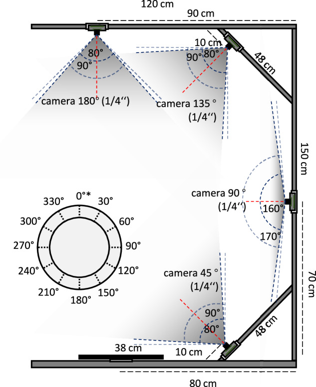 Figure 1
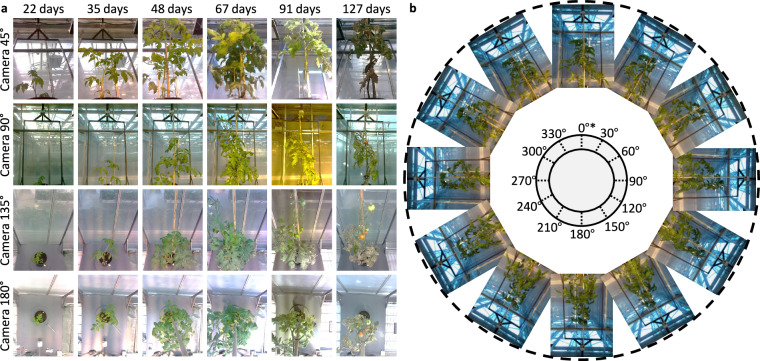 Figure 2
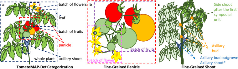 Figure 3
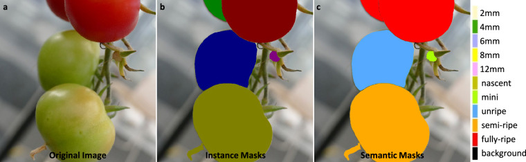 Figure 4
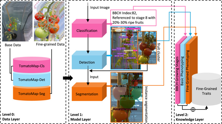 Figure 5
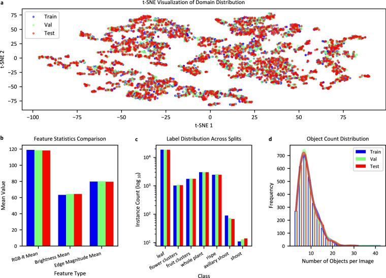 Figure 6
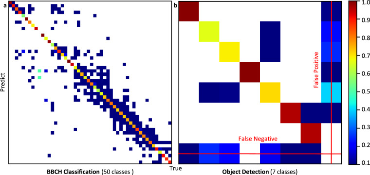 Figure 7
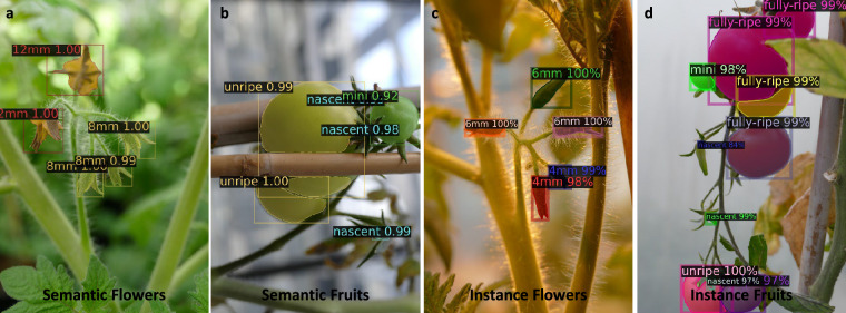 Figure 8
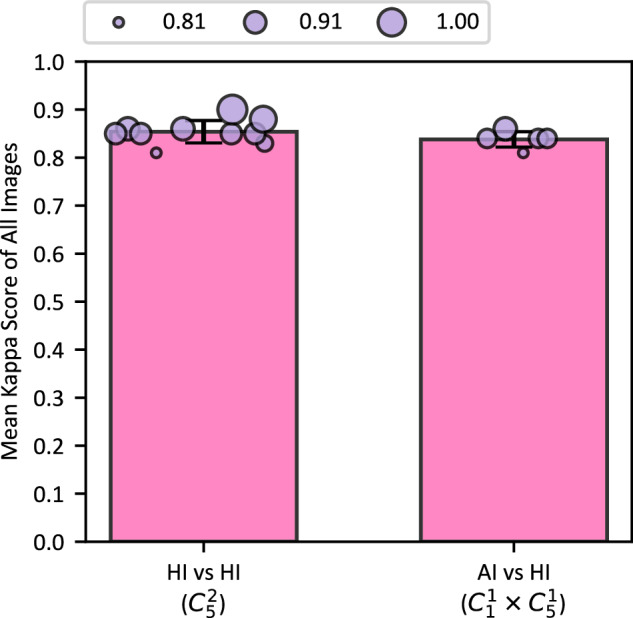 Figure 9
Peer Reviews
No public reviews on file for this paper yet. If you reviewed it on a platform where reviews are public (OpenReview, ICLR, NeurIPS, ICML), you can paste yours below so the community can read it here.
Videos
No videos yet. Explain this paper in a talk, walkthrough, or lecture? Add one.
Taxonomy
TopicsSmart Agriculture and AI
Background and Summary
Solanum lycopersicum (tomato), originating in the Andean region, constitutes a crop of agronomic and economic importance. Following its introduction to Europe in the 16th century, it has reached global dissemination and is now widely cultivated in various agroecological zones^1^. Worldwide, S. lycopersicum is important in the food supply chain and has significant implications for developmental biology, stress biology, and food science^2^. In 2024, the total production of S. lycopersicum for fresh consumption in Europe is 6,671,000 tonnes^3^. Moreover, S. lycopersicum has been firmly established as a model organism within the Solanaceae family and is widely recognized in the field of plant physiology^4^. This status is based on the availability of the fully sequenced and annotated genome along with an extensive repository of genetics, physiological and biochemical data^5^.
As a widely studied model plant, the accurate and high-resolution phenotyping is crucial for hypothesis-driven inquiries and the selection of agronomically desirable genotypes based on traits such as fruit quality, plant architecture, and disease resistance^2,6^. It also supports the dissection of complex trait architectures and advances marker-assisted and genomic selection, as well as the evaluation of responses to abiotic stresses, including drought, heat, and nutrient deficiencies^7^. Additionally, S. lycopersicum exhibits a remarkable degree of phenotypic plasticity^8^, reflected in the extensive variability observed across several agronomical important traits such as fruit size and coloration, flower development, leaf morphology, and sympodial shoot structure^9^. For example, the variation in fruit coloration serves as an optimal trait that provides an ideal feature for developing algorithms capable of accurate color segmentation, the diversity in fruit size and flower stage offers a resource for researching statistics models focused on robust size recognition and classification^10^. This phenotypic diversity provides exceptionally rich and varied scientific information for research aimed at improving fruit productivity, fruit quality^11^, and resilience to environmental stress^12^.
Due to subtle phenotypic variation in S. lycopersicum, advanced imaging and AI-driven phenotyping are essential for reducing observer bias (see Supplementary Fig. 1), enhancing data accuracy, and expediting breeding through high-throughput, standardized datasets. In recent years, there has been growing interest and demand in using artificial intelligence (AI) to automate the phenotyping process, as traditional methods are often labor intensive, subjective, and unable to scale for large datasets^13^. For example, Tian et al.^14^ reported a lightweight detection method for real-time tomato monitoring using edge computing devices and modified different structures of the “You Only Look Once” (YOLO) model. Lee et al.^15^ proposed a clip-type IoT camera based tomato phenotyping system for tracking and detecting tomato flowers and fruits using convolutional neural network (CNN). Rahman et al.^16^ presented a Bayesian network based context estimation algorithm for tomato growth phenotyping combining with CNN. Islam and Hatou^17^ established an AI-assisted five-stage tomato growth monitoring system based on CNN. Statistically, Baar et al.^18^ predicted fruit growth based on tomato diameter from 2D image and environment data with the sigmoid function and its extensions.
Monitoring data acquisition is integral to research involving S. lycopersicum. This species presents several advantages for the generation of high-resolution, fine-grained scientific datasets. Although structures such as buds, flowers, and axillary shoots may be smaller and less visually distinct, tomato plants remain favorable for imaging under controlled conditions. This can be attributed to the complex structure of their compound leaves^19^ and the agronomic characteristics of fruits^20^, which offer clear features. In recent years, numerous stable and reliable datasets have been published, contributing to plant phenotpying research, shown in Table 1.Table 1. Comparison of published image datasets for tomato research.Dataset NameAuthorResearch ObjectsNumber of Images (in total)Number of Instances (by annotation)Categories (in total)Tomato-Village^21,22^Gehlot et al., 2023Leaf Disease5,067166,8868TomatoOD^23,24^Tsironis et al., 2020Fruit Growth2772,4183PlantVillage^25–27^Hughes and Salathe, 2015Leaf Disease54,30654,30638Laboro Tomato^28^Trigubenko, 2020Fruit Growth8049,7776Tian, Kai Tomato Leaves^29,30^Tian et al., 2022Leaf Disease1,0001,0003Taiwan Tomato Leaves^31^Huang and Chang, 2020Leaf Disease4,9764,9766Maharashtra “Tomato Leaf”^32^Khan et al., 2020Leaf Disease1061065TomatoMAPFine-Grained68,080720,93867
The “Tomato-Village” dataset^21,22^ comprises 5,067 images with subsets for disease detection (variation (a)), multi-class classification (variation (b)), and multi-label classification (variation (c)) tasks. Another notable dataset is the “TomatoOD”^23,24^, which contains 277 images with 2,418 annotated tomato fruit samples of unripe, semi-ripe and fully-ripe classes, enabling the tomato fruit localization and growth stage classification. A published large-scale datasets like the “PlantVillage”^25–27^ contain 54,306 classified instances with 38 classes focuses on leaf disease classification and detection, and the “Laboro Tomato” dataset^28^ contains 804 images of different tomato growth stages for detection and instance segmentation tasks. Kai Tian et al. published a tomato leaf disease dataset and trained three different deep learning network architectures^29,30^. Mei-Ling Huang et al. proposed a dataset “Taiwan tomato leaves” with data augmentation technique^31^. Saiqa Khan et al. presented “Tomato Leaf Dataset” generated with different mobile camera models for leaf disease detection purpose^32^.
However, most existing datasets contain single-pose, single-angle images with varying objects and low average labeled instances per class, limiting their use for high-accuracy model training and restricting analysis to 2D spatial features, see Table 2.Table 2. Statistics of published image datasets for tomato research.Dataset NameMulti-View InformationClassificationDetectionSemantic SegmentationInstance SegmentationTomato-Village^21^^22^× ✓**✓× × TomatoOD^23^^24^× ✓**✓× × PlantVillage^25–27^× ✓**✓× × Laboro Tomato^28^× × ✓✓✓Tian, Kai Tomato Leaves^29,30^× ✓× ✓× Taiwan Tomato Leaves^31^× ✓× ✓× Maharashtra “Tomato Leaf”^32^× ✓× × × TomatoMAP✓✓✓✓✓
In contrast, multi-view information demonstrates significant potential. It facilitates the comprehensive characterization of the 3D phenotypic traits of S. lycopersicum^33,34^, preserving critical structural features such as interleaf distances, stem-leaf angles, and shooting topology. Traditional phenotyping faces challenges such as bias, labor intensity, and inefficiency^35^, especially under complex greenhouse conditions with limited class instances and no 3D structure^34^. To address these limitations, TomatoMAP is introduced as a fine-grained, multi-pose, multi-angle time-series dataset of S. lycopersicum. The resource comprises three subsets: (i) TomatoMAP-Cls for BBCH stage classification^36,37^, (ii) TomatoMAP-Det for object detection across key botanical regions of interest (ROIs), and (iii) TomatoMAP-Seg for pixel-wise semantic and instance segmentation.
Methods
Data Acquisition System and Data Generation
Plant samples are cultivated under standardized conditions (see Supplementary Information 1). To enable multi-angle multi-pose imaging of S. lycopersicum, a scalable data acquisition station is first developed. It integrates a synchronized multi-camera array with a rotational platform, facilitating systematic and repeatable image capture across both spatial and temporal dimensions, see Fig. 1.Fig. 1. Data acquisition system, using an imaging array comprising four camera modules. The array provides a composite field of view, incorporating three modules with a 90° diagonal field of view and one module with a 170° diagonal field of view, positioned at vertical inclination angles of 45°, 90°, 135°, and 180° respectively. A turntable with 30° rotational increments is used for multi-pose purpose. To ensure consistent imaging poses for the same plant at different time points, an initial imaging pose position is marked on the tray (denoted as “*” in the figure).
The imaging station comprises four OV5647 color CMOS 5-megapixel image sensors: three are equipped with 90^°^ lenses and one is equipped with a 170^°^ fisheye lens. These cameras are mounted at vertical inclination angles of 45^°^, 90^°^, 135^°^, and 180^°^, each with manual focus and an aperture of f/2.2. The three 90^°^ lenses provide fields of view of 90^°^ (diagonal) and 72^°^ (horizontal), while the 170^°^ fisheye lens offers ultra-wide 170^°^ (diagonal) coverage, allowing comprehensive coverage of the entire plant structure at close range (≈80c**m)^38^.
In total, the modest resolution subset contains phenotypic imaging data gathered over a 163-day period, from August to January. Data acquisition is performed with irregular intervals ranging from 1 to 13 days to adapt to different tomato growth rates and growth dynamics. The dataset comprises images from 101 individual plants, with a total of 32 acquisition time points. At each acquisition time point, plants are placed on the turntable and imaged at 30^°^ rotational increments, resulting in a comprehensive 360^°^ visual dataset. This yields 48 images per plant at each time point, covering multiple poses and angles. All camera modules record images at a resolution of 1080 × 1440 pixels and are synchronized to capture frames at each rotational step (see Fig. 2). This configuration ensures consistent sparse posed multi-view imaging, showing potential for 3D reconstruction and high-fidelity morphological analysis. Using this data acquisition system, a total of 64,464 images are captured and annotated for classification (TomatoMAP-Cls) and object detection (TomatoMAP-Det). The image and annotation files are formatted as Supplementary Information 2. Camera calibration is conducted using a planar chessboard pattern to estimate intrinsic and extrinsic parameters, including lens distortion coefficients. Calibration relied on the detection of 2D corner points and the formation of 3D-to-2D correspondences, following established photogrammetric methods^39^.Fig. 2. Dataset overview. (a) Multi-angle time series protocol of 101 plants subjected to varying lighting conditions within a greenhouse environment. Images are captured by cameras with a vertical inclination angles of 45°, 90°, 135°, and 180°, including different time points covering S. lycopersicum growth stages. (b) Multi-pose protocol utilizing a turntable. Sequential imaging of plant poses is achieved by every 30°. A plastic tray with marked initial point (as “*” in figure) is mounted on the turntable.
For semantic and instance segmentation tasks (TomatoMAP-Seg), 3,616 high-resolution macrophotographs are acquired using a Panasonic Lumix DMC-FZ1000 digital camera (Kadoma, Japan) at 3648 × 5472 pixel resolution.
Annotation for Classification, Detection, and Segmentation
For labeling objectives, multiple annotation techniques are employed in parallel to support different computer vision tasks, including image classification, object detection, and semantic and instance segmentation. A comprehensive overview of the annotated categories and the corresponding number of labeled instances is presented in Table 3.Table 3. Labeled instances and fine-grained class summary of TomatoMAP.a) Classification & Detection Label InformationTaskFine-Grained ClassInstance NumberClassification60 ≤ BBCH < 7010,56070 ≤ BBCH < 8029,32880 ≤ BBCH < 9091,120Detectionwhole plant64,626leaf402,763flower clusters23,127fruit clusters37,684panicle53,137axillary shoot1,761shoot319b) Segmentation Label InformationFlower Stages2mm bud2534mm bud6696mm bud6968mm flower31312mm flower296Fruit Stagesnascent588mini266unripe943semi ripe354fully ripe2,135**(a)** TomatoMAP-Cls and TomatoMAP-Det label information. (b) TomatoMAP-Seg label information. BBCH scale^36,37^ is used for fine-grained stage classification. The BBCH index^36,37^ table can be found in Supplementary Table 1.
BBCH-Based Classification
The BBCH scale^36,37^ provides a standardized and widely applicable framework for describing the phenological development of plants, encompassing all stages from germination to senescence. Supplementary Table 1 shows the BBCH scale^36,37^ used for S. lycopersicum. This scale facilitates precise communication in agronomic research, supports the formulation of crop management strategies, and guides the timing of agrochemical interventions. The BBCH scale^36,37^ is adopted as the primary framework for class-label assignment, providing a systematic and biologically consistent representation of developmental stages. Progression between BBCH stages^36,37^ does not necessarily require the complete cessation of the preceding stage; rather, stages may overlap temporally. Features shared across multiple stages should therefore not be interpreted as redundant. Instead, their recurrence enables the model to learn phenological trajectories and to incorporate temporal dynamics of trait expression. This developmental continuity underscores the need for temporally aware classification strategies. The final distribution of the 50 annotated BBCH classes^36,37^ for key phenological stages of S. lycopersicum is presented in Supplementary Table 2.
Progressive Labeling Workflow for Object Detection
A progressive, AI-assisted annotation protocol is implemented to efficiently label the TomatoMAP-Det subset. The workflow began with a manual labeling phase in Label Studio^40^, which is applied to an initial subset of 1,780 images captured from different camera perspectives. This manually annotated dataset is used to train a first assistive deep learning model. That model is then deployed to produce preliminary labels for an additional 2,504 images; all predictions are rigorously reviewed and corrected by domain experts and merged with the initial set to train a second assistive model. The second model is applied to a further subset drawn from a larger pool of 6,000 images, after which manual expert validation is again performed. The final assistive model, representing the third iteration, is trained using the cumulative annotations from all previous subsets. As a final quality-control step, all annotation files are cross-checked by five experts. At every phase, the image subsets are balanced across camera perspectives to ensure representation consistency.
To ensure high-quality annotations, a rigorous quality-control protocol is implemented. Bounding boxes tightly enclose each target object. For partially visible objects, annotators draw boxes that cover all visible regions together with the morphologically plausible occluded extent, providing consistent representations under varying degrees of occlusion. Objects with extremely limited visible regions, where the structural outline cannot be reliably inferred, are left unannotated, even if they are observable from other viewpoints.
Given the structural complexity of plants, overlap between different classes is permitted, whereas intra-class overlap exceeding 70% is prohibited to avoid redundancy. Adjacent independent objects are individually annotated to maintain granularity. Annotation consistency is maintained across the entire dataset through a three-step verification process: self-inspection by annotators covering all samples, random sampling review of at least 10% of annotations by senior annotators, and cross-validation among different annotators to minimize subjective bias and ensure inter-annotator agreement.
All annotations strictly adhere to predefined class taxonomies. They are defined according to botanical principles in consultation with domain experts.
For fine-grained object detection, the annotation mainly focused on seven biologically relevant ROIs: whole plant, leaf, panicle, flower clusters, fruit clusters, shoot, and axillary shoot. The biological definitions are shown in Fig. 3. Significantly, the axillary shoot grows out of an axillary bud, which also has the potential to develop a flower and fruit clusters. Given the structural complexity of tomato plants, especially in the context of overlapping reproductive structures, annotations for panicle-related classes may involve intersecting regions when multiple fruit or flower clusters coexist within the same inflorescence.Fig. 3. TomatoMap-Det annotation protocol. (a) TomatoMAP-Det categorization. Different ROIs are labeled using rectangular bounding boxes. It’s important to note that certain classes may have overlapping relationships. The pot is excluded from the “whole plant”. (b) Fine-grained panicle. The panicle class encompasses the flower cluster class and the fruit cluster class. The bounding box can overlap in the situation when multiple clusters of flower or fruit grow on the same panicle. (c) Fine-grained shoot phenotypes, including the difference of an axillary shoot, an axillary bud, and a side shoot. Axillary buds have the potential to develop into new shoots, maturing into either axillary shoot or a flower cluster, marked in figure with (*).
Annotation for Fine-Grained Semantic and Instance Segmentation
To facilitate the development of high accuracy model for fine-grained semantic and instance segmentation, a comprehensive annotation protocol is implemented. This protocol involves the labeling of TomatoMAP-Seg, using pixel-wise masks. The annotation process is structured according to the semantic index depicted in Supplementary Fig. 2. This index is referenced from the developmental stages of S. lycopersicum flowers and fruits^41^.
The semantic classes for floral structures are defined based on length measurements, with categories corresponding to 2 mm, 4 mm, 6 mm, 8 mm, and 12 mm. The fruit development stages are categorized based on colorimetric and morphological criteria, comprising five classes: nascent, mini, unripe, semi-ripe, and fully ripe. Following these criteria, the domain experts have been engaged in the interactive annotation workflow that integrates automated segmentation proposals with manual refinement to ensure high labeling fidelity across TomatoMAP-Seg. The annotation is performed using the Interactive Semi-Automatic Annotation Tool (ISAT)^42^ with Segment Anything Model 2 (SAM2)^43^.
An overview of the annotation workflow is shown in Fig. 4. Each labeled instance includes pixel-wise segmentation masks and unique instance identifiers, supporting both semantic and instance segmentation tasks.Fig. 4. TomatoMap-Seg annotation. Semantic and instance masks showing in different colors following the semantic protocol. A pixel-wise labeling process is proposed. Masks are also labeled by instance IDs and class IDs. (a) The original image. (b) Visualization of labeled instance segmentation masks, each individual color references an individual instance. (c) Visualization of labeled semantic segmentation masks, same color instances belong to same class.
Cascading Structure
A three-level cascading structure is proposed to support efficient fine-grained phenotyping, comprising data layer cascading (Level 0), model layer cascading (Level 1), and knowledge layer cascading (Level 2). At the data layer, TomatoMAP is structured in a sequential pipeline. Data are progressively refined according to the granularity requirements and task specifications at each stage. At the model layer, a progressive specialization strategy is introduced, whereby increasingly refined models are employed to enhance specificity and efficiency. This design enables effective resource utilization and facilitates parallel processing of multiple images. At the knowledge layer, comprehensive fine-grained phenotypic data are integrated and centrally validated. The overall structure is depicted in Fig. 5. The cascading strategy mitigates performance degradation across the phenotyping pipeline by limiting error propagation between stages^44^. Furthermore, the modular structure allows each component to be validated independently, thereby improving robustness and maintainability.Fig. 5. TomatoMAP cascading structure. Level 0 shows the upstream cascading data structure. In detail, TomatoMAP-Cls is the subset for classification, TomatoMAP-Det is the subset for detection, and TomatoMAP-Seg for instance and semantic segmentation. Level 1 shows the streamline of cascading model structure. A progressive specialization strategy is introduced, employing increasingly refined models. The input for segmentation model is cascaded with the output from detection model, the detection model select the ROI from interested plants’ growth stages based on the BBCH index classified by classification model. Finally, all the knowledge forms the final fine-grained phenotypic traits at level 2.
FAIR Principles and Domain Shift Analysis
In contrast to many current efforts that focus primarily on scholar-centered data access, the FAIR guiding principles^45^ underscore the importance of machine-friendly data, allowing automated discovery, access, interoperability, and reuse. Such capabilities are essential in our cascading structure, where layered processing is highly dependent on efficient data flow and reusability. Accordingly, the dataset is designed in alignment with these principles to support the requirements of automated, cascading workflows and to maximize its utility within such environments.
To ensure full experimental reproducibility, TomatoMAP-Cls (classification), TomatoMAP-Det (detection), and TomatoMAP-Seg (segmentation) are partitioned into training (70%), validation (20%), and test (10%) subsets using a fixed random seed. For TomatoMAP-Cls, stratified sampling at the class level is employed prior to random selection, yielding 45,099 training, 12,870 validation, and 6,495 test images. TomatoMAP-Det is split using simple random mixed sampling, resulting in 45,124 training, 12,892 validation, and 6,448 test samples. TomatoMAP-Seg, which currently contains 727 annotations, is proportionally divided into 508 training, 146 validation, and 73 test samples. To mitigate class and stage imbalance during dataset construction, images are acquired across diverse developmental stages.
To evaluate the balance of the resulting splits, 3,000 images are randomly sampled from each subset and a t-SNE based domain distribution analysis is conducted over color (RGB), brightness, edge statistics, texture, frequency-domain descriptors, label distributions, and object-count distributions, shown as Fig. 6.Fig. 6. Domain shift analysis across 3,000 standardized samples from training, validation, and test splits with fixed random seed. (a) t-SNE visualization of feature space distribution showing the relationship between train (blue), validation (green), and test (red) splits (perplexity: 30, max optimization iteration: 1,000). (b) Statistical comparison of selected examples of visual features (RGB-R mean, brightness mean, edge magnitude mean) across splits. (c) Class instance distribution on logarithmic scale, showing relative frequencies of all seven tomato plant classes, as well as their balance across spilts. (d) Distribution of objects per image across splits.
In Fig. 6a, the t-SNE visualization demonstrates substantial overlap among the three splits, indicating minimal domain shift and consistent data distribution. Fig. 6b shows the statistical analysis of visual features reveals comparable values for RGB-R, brightness, and edge magnitude across all splits, confirming uniform image characteristics. Fig. 6c presents a balanced representation of all seven tomato plant organ classes across splits, despite an overall class imbalance. The object count distribution exhibits nearly identical patterns across splits, as shown in Fig. 6d.
Data Records
Dataset is deposited in e!DAL (electronic data archive library) of IPK (Leibniz Institute of Plant Genetics and Crop Plant Research): 10.5447/ipk/2025/14^46^. The repository contains two main folders:
- “metadata” contains supporting information of TomatoMAP, including comprehensive manual and semi-automatic phenotypic data for 101 tomato plant samples as well as hardware meta data in CSV files. The dataset includes growth measurements, developmental stage tracking, imaging metadata, and related information.
- “TomatoMAP” folder contains the image data and annotations. The image data is organized into time-series groups. We recommend using our preprocessing scripts to construct the classification and detection datasets. Segmentation annotations can be found directly under the subfolder “TomatoMAP-Seg”.
Technical Validation
TomatoMAP is validated across three computer vision tasks: fine-grained BBCH-based phenological stage classification^36,37^, multi-object detection for ROI localization, and instance segmentation for precise pixel-level delineation.
Given the generic cascading structure described in section Cascading Structure, models balancing high accuracy with computational efficiency are prioritized to enable real-time inference, a primary objective for TomatoMAP. Accordingly, the stage-wise selections are as follows: for BBCH-based classification, MobileNetv3 Large is employed^47,48^ as a lightweight CNN backbone optimized for efficient and fast feature extraction. For object detection, YOLOv11 Large is adopted^49^, leveraging the CSPDarknet backbone^50^ for efficient multi-scale feature extraction. For instance segmentation, Mask R-CNN with a ResNet-50 backbone and Feature Pyramid Network (FPN) is used^51–53^ to achieve precise pixel-level delineation via deep hierarchical features. To support alternative application objectives, evaluation results for additional classification, detection, and segmentation models, as well as reference results using an inverse-frequency data-balancing method, are provided in the Supplementary Information 7 (see also Fig. 5).
To evaluate the model performance, normalized confusion matrices are generated for both classification and detection tasks, using the validation subsets of TomatoMAP-Cls and TomatoMAP-Det (see Fig. 7). The hyperparameter fine-tuning for YOLOv11 Large^49^ and technical details are shown in Supplementary Information 8. The matrices provide a visible quantitative evaluation of the model’s ability to classify between BBCH-based phenological stages and to detect multiple ROIs.Fig. 7. Normalized confusion matrix from MobileNetv3^47,48^ and YOLOv11 Large^49^ on TomatoMAP-Cls and TomatoMAP-Det. (a) Validation of BBCH classification for MobileNetv3 Large model^47,48^ with 50 classes^36,37^. Since the BBCH scale^36,37^ is originally designed as a general plant growth stage index, for some plants, certain stages may be skipped. Consequently, the BBCH index^36,37^ shown in this figure does not exhibit a linear relationship with phenological distances between growth stages, since TomatoMAP-Cls includes only a partial representation of the original BBCH scale^36,37^, for example the seedling stage. Based on the data annotation, where only 50 indexes are used, index jumping can appear. White areas inside the matrix refer to 0. Error fluctuation occurs due to the similarities between classes. (b) Validation of object detection for fine-tuned YOLOv11 Large^49^ for seven classes. By column normalization, the last bottom row shows the false negative detections, and the last right column shows the false positive detections.
In Fig. 7a, class imbalance and subtle differences between classes lead to misclassifications that appear near the diagonal, reflecting the biological complexity and visual similarity of adjacent BBCH stages. A manual classification of such stages is labor-intensive and prone to error. Fig. 7b shows strong diagonal dominance in the detection results, particularly for the leaf, whole plant, and shoot categories. However, classes such as flower and fruit clusters, as well as panicles, show elevated rates of false positives and false negatives, indicating areas requiring further refinement.
Figure 8 visualizes segmentation outcomes at the flowering and fruiting stages: Subfigures (a) and (b) present semantic segmentation results. Items of the same mask color belong to the same semantic category. Subfigures (c) and (d) present instance segmentation outputs. Each instance is color-coded individually, with its confidence score and category label displayed in the top-left corner of the bounding box. The model performance is particularly strong for unripe, semi ripe and fully ripe fruits, as well as flowers exceeding 4 mm in length. In contrast, the performance declines for early-stage classes such as nascent fruits and 2 mm buds, highlighting the challenge of detecting smaller, low-contrast objects.Fig. 8. Examples from the prediction results with 0.5 confidence under different scenes. Sub-figures (a) and (b) display semantic segmentation results for clusters of flower and fruit, respectively, with the class name and confidence labeled at the top-left of each bounding box. Items of the same mask color belong to the same semantic category. Sub-figures (c) and (d) present instance segmentation results, where individual flowers and fruits are masked in different colors. The confidence score for each instance is displayed in the top-left corner of its corresponding bounding box.
Overall, these results highlight TomatoMAP-Seg’s effectiveness in capturing fine-grained morphological traits throughout reproductive development, supporting its utility for downstream phenotypic analysis in plant research.
To quantitatively evaluate the inter-rater agreement^54^ between human annotators and AI, two complementary methods are employed: Cohen’s Kappa^55^ and inter-rater agreement heatmaps^54^. Cohen’s Kappa^55^ is utilized to measure the statistical agreement between pairs of annotators, while inter-rater agreement heatmaps^54^ provide an intuitive visualization of spatial annotation consistency across the pixel domain (see Supplementary Information 3).
Cohen’s Kappa^55^ is calculated for each pairwise combination of annotators, including comparisons between human experts and AI model, where Po is the observed agreement and Pe is the expected agreement due to chance. The kappa score is defined as:
\documentclass[12pt]{minimal} \usepackage{amsmath} \usepackage{wasysym} \usepackage{amsfonts} \usepackage{amssymb} \usepackage{amsbsy} \usepackage{mathrsfs} \usepackage{upgreek} \setlength{\oddsidemargin}{-69pt} \begin{document}$$\kappa =\frac{{P}_{o}-{P}_{e}}{1-{P}_{e}},$$\end{document}The value of kappa score ranges from -1 (complete disagreement) to 1 (perfect agreement), where 0 indicating no better agreement than random chance. The interpretation of the κ values follows established guidelines^56,57^, as detailed in Supplementary Table 6. The analysis pipeline starts with pre-processing and deduplication. Each annotator’s YOLO-format labels are preprocessed first by iterating over all the bounding boxes. Highly overlapping bounding boxes of semantically related classes (e.g. flower clusters, fruit clusters, and panicle) are merged to reduce inter-rater redundancy. To accommodate minor spatial discrepancies in object localization and to associate bounding boxes produced by different annotators, for example, slight positional offsets for the same semantic instance, an Intersection-over-Union (IoU) based matching algorithm is employed. Box pairs are matched only if their IoU threshold θ exceeds a given threshold, e.g. θ ≥ 0.5. Then Cohen’s Kappa^55^ is computed between five domain experts for human intelligence (HI) comparison (HI vs HI, \documentclass[12pt]{minimal} \usepackage{amsmath} \usepackage{wasysym} \usepackage{amsfonts} \usepackage{amssymb} \usepackage{amsbsy} \usepackage{mathrsfs} \usepackage{upgreek} \setlength{\oddsidemargin}{-69pt} \begin{document}$${C}_{5}^{2}$$\end{document} ) and between AI model and each expert (AI vs HI, \documentclass[12pt]{minimal} \usepackage{amsmath} \usepackage{wasysym} \usepackage{amsfonts} \usepackage{amssymb} \usepackage{amsbsy} \usepackage{mathrsfs} \usepackage{upgreek} \setlength{\oddsidemargin}{-69pt} \begin{document}$${C}_{1}^{1}\times {C}_{5}^{1}$$\end{document} ) for 295 images external to TomatoMAP. Results are shown in Fig. 9.Fig. 9. Comparison between human and an AI model trained with TomatoMAP. Mean Cohen’s kappa score for all images for each experimental pair. By calculating the Cohen’s kappa between five domain experts (HI vs HI, \documentclass[12pt]{minimal} \usepackage{amsmath} \usepackage{wasysym} \usepackage{amsfonts} \usepackage{amssymb} \usepackage{amsbsy} \usepackage{mathrsfs} \usepackage{upgreek} \setlength{\oddsidemargin}{-69pt} \begin{document}$${C}_{5}^{2}$$\end{document} ) and between AI model and each expert (AI vs HI, \documentclass[12pt]{minimal} \usepackage{amsmath} \usepackage{wasysym} \usepackage{amsfonts} \usepackage{amssymb} \usepackage{amsbsy} \usepackage{mathrsfs} \usepackage{upgreek} \setlength{\oddsidemargin}{-69pt} \begin{document}$${C}_{1}^{1}\times {C}_{5}^{1}$$\end{document} ) for 295 images external to TomatoMAP, we feature the mean Cohen’s kappa based on each experiment pair. The “HI vs HI” group exhibit “almost perfect agreement” between experts, while the “AI vs HI” group shows the same agreement.
Based on Cohen’s Kappa coefficient^56,57^, “HI vs HI” groups exhibit “almost perfect agreement” between experts, while the “AI vs HI” group shows the same agreement. The inter-rater agreement heatmaps (see Supplementary Fig. 1) further demonstrated the concordance of human annotations in regions of biological relevance. Moderate disagreement in peripheral regions is likely attributable to subjectivity in boundary delineation, particularly in the absence of clear anatomical landmarks. Without importing stochastic layers, augmentation, and other random parameters, YOLOv11^49^ model trained with TomatoMAP demonstrated high internal consistency across inference replicates, offering a significant advantage over human annotators, whose performance typically exhibits variability.
The result proves the high alignment of AI and human in phenotyping task and underscore the potential of AI-assisted phenotyping in eliminating bias, reducing the time and labor costs of manual phenotyping.
Limitations
Owing to intrinsic biological characteristics of tomato plants, specifically the lower prevalence of flower and fruit clusters relative to leaves, achieving balanced annotations and AI-human performance comparison across organ classes are challenging. Although the inverse frequency weighting algorithm improves overall model performance, certain classes remain undertrained. Moreover, within the proposed cascading structure, practical criteria for selecting models that optimally balance performance against constraints of real time deployment remain insufficiently established. Future research will focus on developing models constrained by GFLOPs and computational resources of individual edge devices, while enhancing parallel processing efficiency and obtaining high-quality fine-grained phenotypic data.
Supplementary information
Supplementary information
The reference list from the paper itself. Each links out to its DOI / PubMed record.
- 1European Commission, Eurostat. Production of tomatoes for fresh consumption. European Commissionhttps://agridata.ec.europa.eu/extensions/Dashboard Fruit And Veg/Fruitand Vegetable Production.html (Accessed 28 April 2025).
- 2Kimura, S. & Sinha, N. Tomato (Solanum lycopersicum): A Model Fruit-Bearing Crop. CSH Protocols 2008, pdb.emo 105 10.1101/pdb.emo 105 (2008).10.1101/pdb.emo 10521356708 · doi ↗ · pubmed ↗
- 3Jana, S. & Parekh, R. Shape-based Fruit Recognition and Classification. In Computational Intelligence, Communications, and Business Analytics (eds Mandal, J. K., Dutta, P. & Mukhopadhyay, S.) Communications in Computer and Information Science 776, 184–196 (Springer Singapore, 2017).
- 4Gehlot, M., Saxena, R. K. & Gandhi, G. C. “Tomato-Village”: a dataset for end-to-end tomato disease detection in a real-world environment. Githubhttps://github.com/mamta-joshi-gehlot/Tomato-Village.
- 5Tsironis, V., Bourou, S. & Stentoumis, C. tomat OD: Evaluation of object detection algorithms on a new real-world tomato dataset. Githubhttps://github.com/up 2metric/tomat OD.
- 6Hughes, D. P. & Salathé, M. An open access repository of images on plant health to enable the development of mobile disease diagnostics through machine learning and crowdsourcing. ar Xiv preprint https://arxiv.org/abs/1511.08060 (2015).
- 7Mohanty, S. P., Hughes, D. P. & Salathé, M. Using deep learning for image-based plant disease detection. Frontiers in Plant Science 710.3389/fpls.2016.01419 (2016).10.3389/fpls.2016.01419 PMC 503284627713752 · doi ↗ · pubmed ↗
- 8Mohanty, S. P., Hughes, D. P. & Salathé, M. Using deep learning for image-based plant disease detection. Githubhttps://github.com/sp Mohanty/Plant Village-Dataset.10.3389/fpls.2016.01419 PMC 503284627713752 · doi ↗ · pubmed ↗