Mortality risk during the COVID-19 pandemic is shaped by human development
Kolja Nenoff, Sarah Habershon, Miguel D. Mahecha, Sabine Attinger, Khalil Teber, Guido Kraemer

TL;DR
The study shows that socioeconomic factors, not just reported cases, strongly influence pandemic mortality, using machine learning to uncover hidden patterns.
Contribution
A novel framework using compressed National Framework Conditions (cNFCs) better explains pandemic mortality than traditional metrics.
Findings
The machine learning model explained nearly half of global excess mortality variance.
cNFCs had a stronger impact on mortality predictions than reported case numbers.
Socioeconomic factors like labor force age and health spending shaped mortality outcomes.
Abstract
During the global COVID-19 pandemic (2020–2021), excess mortality varied substantially across countries. Notably, upper-middle-income countries experienced greater variability in excess mortality than both low- and high-income countries, despite reporting fewer COVID-19 cases than high-income countries but more than low-income countries. This disconnect between case numbers and mortality suggests more complex structural vulnerabilities. Socioeconomic conditions and healthcare system performance, collectively referred to as National Framework Conditions (NFCs), are likely key determinants of pandemic outcomes. However, the specific relationship between these factors and excess mortality remains poorly understood. We constructed a predictive model of excess mortality using reported COVID-19 case counts and a wide array of NFCs derived from the World Development Indicators (WDI),…
Genes, proteins, chemicals, diseases, species, mutations and cell lines named across the full text — each resolved to its canonical identifier and authoritative record.
Click any figure to enlarge with its caption.
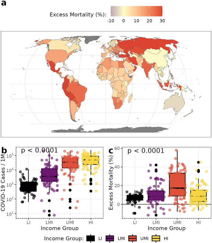 Figure 1
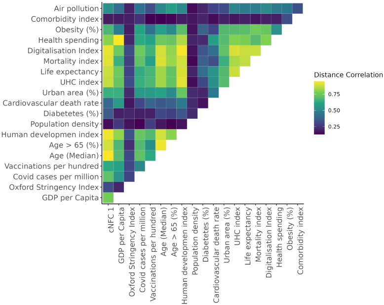 Figure 2
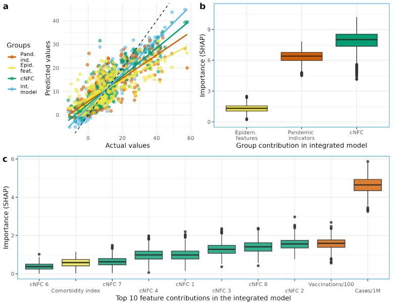 Figure 3
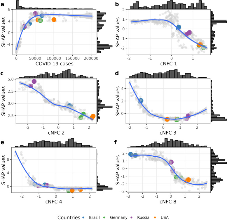 Figure 4
- —https://doi.org/10.13039/501100001656Helmholtz-Gemeinschaft
- —Universität Leipzig (1039)
Peer Reviews
No public reviews on file for this paper yet. If you reviewed it on a platform where reviews are public (OpenReview, ICLR, NeurIPS, ICML), you can paste yours below so the community can read it here.
Videos
No videos yet. Explain this paper in a talk, walkthrough, or lecture? Add one.
Taxonomy
TopicsCOVID-19 epidemiological studies · COVID-19 and healthcare impacts · COVID-19 Clinical Research Studies
Background
The COVID-19 pandemic’s impact on excess mortality varied widely across countries and regions, often showing patterns that did not align with reported case numbers. By the end of 2021, the number of deaths directly attributed to COVID-19 reached approximately 5.4 million globally, while estimates of excess mortality ranged from 12 to 22 million [1–5]. These excess deaths were unevenly distributed, with particularly high rates observed in Latin America and countries of the former Soviet bloc, and comparatively lower rates in Oceania and parts of Africa (Fig. 1a).
Reported COVID-19 cases in 2020–2021 followed a gradient corresponding to countries’ income group (Fig. 1b). However, excess mortality in upper-middle-income countries was higher than in low- or high-income countries (Fig. 1c) [6, 7]. The reasons behind cross-country differences in COVID-19 health outcomes remain the subject of ongoing debate [8, 9]. Neither viral exposure measured through reported COVID-19 cases nor containment policies, such as non-pharmaceutical interventions, adequately account for the observed variation in excess mortality across countries [10, 11]. Excess mortality refers to the difference between the total number of observed deaths and the number expected under normal conditions. The World Health Organization (WHO) provides globally harmonized estimates of excess mortality based on this definition, expressed as the percentage difference between observed and expected all-cause deaths (P-score excess mortality) [1]. It captures both direct deaths from COVID-19 and indirect deaths arising from the broader effects of the pandemic, such as disruptions to healthcare and social systems [12]. As such, excess mortality provides a more robust and comprehensive measure of the pandemic’s true health outcome [13].
In addition to measuring outcomes, we must account for differences in exposure to the virus, which may confound the relationship between socioeconomic conditions and excess mortality. To represent this exposure, a consistent and globally available covariate is required. Readily accessible indicators include reported COVID-19 cases and deaths, both of which are affected by reporting biases arising from different processes. COVID-19 case data are generally compiled using simpler and more standardized criteria, primarily reflecting testing and surveillance capacity, whereas COVID-19 death data depend on cause-of-death certification, medical review, and registration systems that vary widely across countries. The question of how to measure population exposure remains a topic of ongoing debate, with different approaches involving trade-offs between data availability and comparability across countries [14–18]. We use reported COVID-19 cases as a practical proxy for exposure and excess mortality as the outcome variable, acknowledging that both indicators are influenced by underreporting and measurement limitations.
A growing body of evidence suggests that socioeconomic and demographic structure, collectively termed National Framework Conditions (NFCs), were key drivers of this gap, particularly in middle-income countries [19–22]. Yet most studies assess these conditions using individual indicators, such as gross domestic product (GDP), prevalence of respiratory diseases, or healthcare spending without accounting for their interactions or structural configurations, such as the relationship between median population age and healthcare expansion [8, 23–27]. These univariate or additive models may obscure the systemic nature of pandemic vulnerability.
Understanding these systemic vulnerabilities is essential to examine how the risks countries face are structured through their socioeconomic and institutional conditions. The purpose of this analysis is to identify and characterize the coping capacity of countries within this structural context, positioning pandemic response as part of a broader system of national resilience. By linking these conditions to health outcomes, we aim to reveal the underlying configurations that shaped the pandemic’s unequal impact and to provide insights for strengthening resilience and reducing vulnerability to future global risks.Fig. 1. Global Patterns of COVID-19 Cases and Excess Mortality. a Illustrates the geographical distribution of mean annual excess mortality for 2020–2021 (capped at 95^th^ percentile for visualization). b and c show the distribution of COVID-19 cases and excess mortality, respectively, stratified by World Bank income classifications. Statistical differences between income groups were assessed using Kruskal-Wallis tests. Data points in panels b and c represent country-year observations for 173 countries (n = 346 for 2020–2021). Colors correspond to the World Bank country income classifications: low income (LI), lower-middle income (LMI), upper-middle income (UMI), and high income (HI). Data sources: WHO [1] for excess mortality, Our World in Data [6] for COVID-19 cases, and World Bank [28] for income classifications
To overcome the limitations of these models, we propose a new approach. We jointly analyze a broad set of socioeconomic, demographic, and structural indicators from the WDI database comprising 1477 dimensions. Recognizing that development is nonlinear and context-dependent, we use a nonlinear dimensionality reduction method (e-Isomap) to project these variables into a low-dimensional latent space. This latent representation, which we call compressed National Framework Conditions (cNFCs), captures the essential variation in development structures while preserving their non-linear relationships [29, 30].
We use these cNFCs as input to a machine learning model that predicts excess mortality, alongside controls for pandemic exposure and known epidemiological risk factors. SHAP (SHapley Additive exPlanations) values allow us to quantify the relative contributions of socioeconomic structures, pandemic indicators (such as reported cases), and traditional health risk metrics to the model’s predictions of excess mortality. While the model is constrained by data availability and reflects associations rather than causal mechanisms, it provides a coherent and interpretable framework for assessing how national conditions shaped the global toll of the pandemic and may inform preparedness for future health crises.
Methods
This study aims to identify how socioeconomic conditions contribute to the gap between reported COVID-19 case counts and observed excess mortality. To close this gap, we assemble data from three key domains: socioeconomic, pandemic indicators, and epidemiological features.
We begin by introducing excess mortality as our dependent variable, comparing estimates from multiple sources to justify our choice. Next, we present our socioeconomic data, drawn from the WDI, and describe our approach to compressing this high-dimensional dataset into a smaller set of interpretable components referred to as cNFCs. Based on previous work, these latent dimensions are characterized in terms of their thematic and structural properties [30].
In addition, we include a wide set of epidemiological features and pandemic indicators as control variables, including reported COVID-19 cases per million, Vaccinations per hundred, the Oxford Coronavirus Government Response Tracker stringency Index (Oxford stringency index), and other known risk factors (Table 1).
All components are integrated into a predictive machine learning model. This framework allows us to quantify the unique contribution of the cNFCs to excess mortality, while controlling for pandemic factors. We estimate the predictive influence of each variable using interpretable machine learning techniques (SHAP values). This SHAP values reveal which variables are important, providing insight into how structural and dynamic factors jointly shaped pandemic outcomes.
Excess mortality data
We used the P-score of the excess mortality as our outcome variable, as defined by the WHO. The P-score is the percentage difference between observed and expected all-cause mortality. Importantly, it includes both direct deaths from COVID-19 and indirect deaths resulting from disruptions to healthcare systems, social services, and economic activity [1, 12].
As a health outcome metric, excess mortality is robust and less prone to biases than reported COVID-19 deaths, which can vary significantly across countries due to differences in case definitions, diagnostic capacity, reporting infrastructure, and cause-of-death attribution [13, 31–33].
Many excess mortality estimates have been published [1, 2, 7, 9]. The two most prominent, which we compared, show high similarities between the estimated values per country (Supplementary Material 1: Chapter S2 and Supplementary Material 1: Fig. S1). However, they differ in coverage and methods. We choose the WHO’s excess mortality estimates for 2020–2021 due to their broad global coverage (194 countries) and standardized methodology [1].
The WHO’s representation of excess mortality as a P-score (see Eq. 1) allows for meaningful cross-country comparisons by accounting for population size and baseline mortality rates.
\documentclass[12pt]{minimal} \usepackage{amsmath} \usepackage{wasysym} \usepackage{amsfonts} \usepackage{amssymb} \usepackage{amsbsy} \usepackage{mathrsfs} \usepackage{upgreek} \setlength{\oddsidemargin}{-69pt} \begin{document}$$\begin{aligned} P\text {-score}_{c,t} = 100 \cdot \frac{\text {Reported Mortality}_{c,t} - \text {Expected Mortality}_{c,t}}{\text {Expected Mortality}_{c,t}} \end{aligned}$$\end{document}In this representation, c denotes a country and t the year. We aggregated P-scores for 2020 and 2021 for all countries available in both the excess-mortality dataset and the WDI. Extreme outliers were defined as values with an interquartile range (IQR), the difference between the 75th and 25th percentiles, more than four times greater than the median ( \documentclass[12pt]{minimal} \usepackage{amsmath} \usepackage{wasysym} \usepackage{amsfonts} \usepackage{amssymb} \usepackage{amsbsy} \usepackage{mathrsfs} \usepackage{upgreek} \setlength{\oddsidemargin}{-69pt} \begin{document}$$\text {IQR}=12.42$$\end{document} , median = 8.96). Following this criterion, Peru’s data for 2020 (P-score = 91.09) and 2021 (P-score = 102.81) were identified as outliers and excluded from further analysis. The final sample comprised P-scores for 174 countries across 2 years ( \documentclass[12pt]{minimal} \usepackage{amsmath} \usepackage{wasysym} \usepackage{amsfonts} \usepackage{amssymb} \usepackage{amsbsy} \usepackage{mathrsfs} \usepackage{upgreek} \setlength{\oddsidemargin}{-69pt} \begin{document}$$n = 348$$\end{document} ).
World development indicators and NFC
The WDI comprises 1477 socioeconomic, environmental, and health-related indicators indicators from 217 countries (1960–2022) [34]. Many of these variables are highly correlated. For instance, “Access to electricity (% of population)” and “Life expectancy at birth, total (years)” are strongly correlated with \documentclass[12pt]{minimal} \usepackage{amsmath} \usepackage{wasysym} \usepackage{amsfonts} \usepackage{amssymb} \usepackage{amsbsy} \usepackage{mathrsfs} \usepackage{upgreek} \setlength{\oddsidemargin}{-69pt} \begin{document}$$dcor = 0.8$$\end{document} . In fact, it has been shown for the WDI data earlier that these data are highly compressible with methods taking the non-linear structure into account [30]. The compressed data lie in a latent space which we will interpret as the cNFCs.
Linear methods, such as principal component analysis (PCA), do not capture the non-linear relationships present in socioeconomic data. To reduce the high dimensionality of the WDI dataset, we applied a non-linear dimensionality reduction technique (Supplement material chapter S2). We used Isomap, a technique that preserves geodesic distances between data points in a lower-dimensional embedding, thereby maintaining the global structure of the original data [29]. Isomap is sensitive to missing data, which is common in global development datasets. We therefore employed a robust variant known as Ensemble Isometric Feature Mapping (e-Isomap) [30]. This method generates multiple geodesic distance matrices from gap-filled subsets of the data and combines them into a stable embedding. This ensemble approach has previously been applied to an earlier version of the WDI. We successfully extended it to a more recent and expanded WDI dataset, enabling a stable and interpretable compression of 1477 socioeconomic indicators to a set of low-dimensional latent variables (cNFCs) (Supplementary Material 1: Fig. S3).
We limited the dataset’s temporal scope to 1990–2021 to maximize data quality and consistency. We also retained only indicators relative to population size (e.g., “Population, female (% of total population)” instead of “Population, female (total)”) and excluded indicators with more than 50% missing values. Despite maximizing data availability, 16% of values are missing. Only for the most developed countries is the data almost complete, while low- and lower-middle-income countries show a high proportion of missing data. We addressed this by limiting the temporal scope with minimum missing values and applying gap-filling procedures [30]. The final dataset before dimension reduction comprises 503 indicators from 180 countries (1998–2021).
The cNFC dimensions
We compressed the WDI dataset into low-dimensional latent space using e-Isomap, which lowers the redundancy and reveals the main structural components of socioeconomic variation (Supplement material S3). This method preserves both linear and non-linear relationships and enables interpretable components, referred to as cNFCs, that can be traced back to the original indicators using the non-linear correlation method energy distance correlation (dcor) [35, 36].
To identify an appropriate dimensionality reduction approach, we compared several methods, including PCA and e-Isomap using different gap-filling strategies. Specifically, we examined how well the low-dimensional data representations could explain excess mortality across countries measured in terms of \documentclass[12pt]{minimal} \usepackage{amsmath} \usepackage{wasysym} \usepackage{amsfonts} \usepackage{amssymb} \usepackage{amsbsy} \usepackage{mathrsfs} \usepackage{upgreek} \setlength{\oddsidemargin}{-69pt} \begin{document}$$R^2$$\end{document} and residual mean squared error (RMSE). Excess mortality itself was not used to construct or tune the cNFCs themselves. We found that e-Isomap with ten dimensions provided the most stable and interpretable representation, and used it throughout the analysis (Supplement material S4).
The cNFCs reflect distinct aspects of national development. In our model we include the most recent representations of ten cNFCs numbered by their amount of explained variance (Supplement Fig. 2a). For reasons of interpretability we are focusing here on describing the ones that will have the highest importance for predicting excess mortality in the analysis later in the paper. The association with the indicators is traced back with energy distance correlation and visualized Supplementary Material 1: Fig. S3.
- cNFC 1 represents 74% of the variance in the WDI dataset (Supplementary Material 1: Fig. S2a) and represents a classic economic-development gradient in which aging populations and declining fertility accompany a transition from agrarian to service-based economies. Consistent with findings by [30], it is strongly correlated with the Human Development Index, and many of the epidemiological features, as shown in Fig. 2. We find that cNFC 1’s middle-range value countries have the highest excess mortality, reflecting a similar non-linear relationship as the World Bank income classifications.
- cNFC 2, which explains 8% of variance in the WDI, reflects structural economic differences, particularly those associated with trade and labor force composition, and the energy intensity of the economy. High values in cNFC 2 indicate economies driven by diversified service sectors. Lower values suggest reliance on primary sectors and manufacturing. cNFC 2 shows countries on the lower end, which are characterized by primary sector and manufacturing dependence than the service-oriented economies.
- cNFC 3 captures aspects of public sector employment and mortality rates, particularly in lower-middle-income countries. It is moderately correlated with “Death rate, crude (per 1000 people)” ( \documentclass[12pt]{minimal} \usepackage{amsmath} \usepackage{wasysym} \usepackage{amsfonts} \usepackage{amssymb} \usepackage{amsbsy} \usepackage{mathrsfs} \usepackage{upgreek} \setlength{\oddsidemargin}{-69pt} \begin{document}$$dcor = 0.69$$\end{document} ) and “Ratio of female to male labor force participation rate (%)” ( \documentclass[12pt]{minimal} \usepackage{amsmath} \usepackage{wasysym} \usepackage{amsfonts} \usepackage{amssymb} \usepackage{amsbsy} \usepackage{mathrsfs} \usepackage{upgreek} \setlength{\oddsidemargin}{-69pt} \begin{document}$$dcor = 0.63$$\end{document} ).
- cNFC 4 covers aspects of economic profiles but is mostly a gradient between regions. High values are associated with the Gulf states such as United Arab Emirates and Kuwait, while low values such as Paraguay and Bolivia are in Latin America.
- cNFC 8 is associated with indicators of public health vulnerabilities and economic reliance on tourism and external aid. High cNFC 8 values are found in countries like Samoa, Vanuatu, and São Tomé and Príncipe. In contrast, low values in Brazil and Colombia. cNFC 8 correlates with “International tourism, receipts (% of total exports)” ( \documentclass[12pt]{minimal} \usepackage{amsmath} \usepackage{wasysym} \usepackage{amsfonts} \usepackage{amssymb} \usepackage{amsbsy} \usepackage{mathrsfs} \usepackage{upgreek} \setlength{\oddsidemargin}{-69pt} \begin{document}$$dcor = 0.35$$\end{document} ), “Incidence of HIV, ages 15–24 (per 1000 uninfected)” ( \documentclass[12pt]{minimal} \usepackage{amsmath} \usepackage{wasysym} \usepackage{amsfonts} \usepackage{amssymb} \usepackage{amsbsy} \usepackage{mathrsfs} \usepackage{upgreek} \setlength{\oddsidemargin}{-69pt} \begin{document}$$dcor = 0.35$$\end{document} ), and “Trade in services (% of GDP)” ( \documentclass[12pt]{minimal} \usepackage{amsmath} \usepackage{wasysym} \usepackage{amsfonts} \usepackage{amssymb} \usepackage{amsbsy} \usepackage{mathrsfs} \usepackage{upgreek} \setlength{\oddsidemargin}{-69pt} \begin{document}$$dcor = 0.34$$\end{document} ), linking this dimension to economies that are vulnerable to external public health challenges and service-based exports.
Pandemic indicators and epidemiological features as covariates
The covariates are grouped into two categories based on their role in the analysis. They are collected from various sources and described in Table 1. Pandemic indicators reflect reported pandemic-related metrics directly linked to the pandemic experience. Epidemiological features are risk factors potentially associated with the excess mortality.
Pandemic indicators represent the key pandemic trajectories. We selected the Oxford Stringency Index, COVID-19 Cases per million, and Total vaccinations per hundred to incorporate government responses, infection prevalence, and population immunity [6, 37]. We also examined the cumulative infection–fatality ratio (IFR) from the IHME to account for differences in age structure and infection ascertainment across countries. After aggregating IFR estimates to annual values, its inclusion did not materially affect model performance or the ranking of the main feature groups, and IFR exhibited low predictive importance. The additional analysis is published in our Github repository. Table 1. Pandemic indicators and epidemiological features considered in the analysis. Data sources include Our World in Data (OWID), State of Global Air report (SGA) and the World Bank World Development Indicators (WDI). HDI denotes the Human Development Index, GDP denotes gross domestic product, PPP purchasing power parity, UHC Universal Health Coverage, and PM \documentclass[12pt]{minimal} \usepackage{amsmath} \usepackage{wasysym} \usepackage{amsfonts} \usepackage{amssymb} \usepackage{amsbsy} \usepackage{mathrsfs} \usepackage{upgreek} \setlength{\oddsidemargin}{-69pt} \begin{document}$$_{2.5}$$\end{document} fine particulate matter with aerodynamic diameter below 2.5 μmVariablesDescriptionData sourcePandemic indicatorsOxford stringency indexOxford stringency indexOWIDCOVID-19 casesNew reported COVID-19 cases per millionOWIDVaccinations per hundredCOVID-19 vaccine doses administered per 100 peopleOWIDEpidemiological featuresLife expectancyLife expectancyOWIDAge>65 (%)Percentage of population older than 65OWIDObesity (%)Prevalence of obesityOWIDAge (Median)Median age of populationOWIDPop densityPopulation densityOWIDDiabetes (%)Prevalence of diabetesOWIDCardio. death rate (%)Cardiovascular death rate in percentOWIDUrbanizationPercent of urban populationOWIDHandwashing facilities (%)Percent of population with access to basic handwashing facilitiesOWIDHDIHuman Development IndexOWIDGDP per Capita (PPP)GDP per Capita adjusted by purchasing power parityWDIAir pollutionYearly average PM \documentclass[12pt]{minimal} \usepackage{amsmath} \usepackage{wasysym} \usepackage{amsfonts} \usepackage{amssymb} \usepackage{amsbsy} \usepackage{mathrsfs} \usepackage{upgreek} \setlength{\oddsidemargin}{-69pt} \begin{document}$$_{2.5}$$\end{document} exposureSGAUHC indexUniversal Health Coverage indexWDIHealth spendingHealth expenditure per capitaWDIHospital bedsHospital beds per thousandOWIDComorbidity indexBurden of disease indicatorsOWID(1)Digitalization indexDigitalization indicatorsWDI(1)Mortality indexMortality of non-natural causesWDI(1)(1) compressed into a single indicator with PCA
Epidemiological features set comprises established epidemiological risk factors such as obesity prevalence [38]. We also incorporated composed indices that might impact the pandemic resilience analog to previous publication [24]. One example Comorbidity Index, which is constructed out of the first principle component (93% explained variance) of the Global Burden of Disease dataset [39].
Feature selection and data preparation
To identify independent features, we tested the correlation between all ten cNFC dimensions, the Pandemic indicators, and the Epidemiological features
We ensured that retained variables contributed distinct and independent information by calculating distance correlation between all features. We excluded 15 variables with a correlation higher than 0.75 and always the one with he lower coverage. We included as many features as possible while maintaining global coverage. For variables with less than 10% missing data, we applied probabilistic PCA for gap filling [40]. Variables with insufficient observations across countries, such as Handwashing Facilities, Cardiovascular Death Rate, and Air Pollution, were excluded from the analysis.
The final feature set used in the model includes 18 variables: ten cNFC dimensions (ordered by the share of WDI variance they explain), three Pandemic indicators (COVID Cases per million, Oxford Stringency Index, and Vaccinations), and five Epidemiological features (Population Density, Urban Area in %, Diabetes Prevalence, Obesity Prevalence, and the Comorbidity Index).
The ten cNFC dimensions were selected using the most recent available values preceding the corresponding P-score for each country-year pair. Accordingly, excess mortality in 2020 was modeled with cNFC values from 2019, and mortality in 2021 with values from 2020. This 1-year lag ensures that a country’s socioeconomic and institutional conditions reflect the situation prior to the pandemic outcomes, avoiding circularity in the analysis.
Our analysis is structured around the three feature domains: pandemic indicators, epidemiological features, and the cNFCs. To ensure independence among variables, we used pairwise distance correlation as a filter. Features with \documentclass[12pt]{minimal} \usepackage{amsmath} \usepackage{wasysym} \usepackage{amsfonts} \usepackage{amssymb} \usepackage{amsbsy} \usepackage{mathrsfs} \usepackage{upgreek} \setlength{\oddsidemargin}{-69pt} \begin{document}$$dcor>0.75$$\end{document} with any cNFC were removed to avoid collinearity. In total, eight epidemiological features were excluded in this step. Notably, median age ( \documentclass[12pt]{minimal} \usepackage{amsmath} \usepackage{wasysym} \usepackage{amsfonts} \usepackage{amssymb} \usepackage{amsbsy} \usepackage{mathrsfs} \usepackage{upgreek} \setlength{\oddsidemargin}{-69pt} \begin{document}$$dcor = 0.94$$\end{document} ), the Human Development Index ( \documentclass[12pt]{minimal} \usepackage{amsmath} \usepackage{wasysym} \usepackage{amsfonts} \usepackage{amssymb} \usepackage{amsbsy} \usepackage{mathrsfs} \usepackage{upgreek} \setlength{\oddsidemargin}{-69pt} \begin{document}$$dcor = 0.93$$\end{document} ), and digitalization ( \documentclass[12pt]{minimal} \usepackage{amsmath} \usepackage{wasysym} \usepackage{amsfonts} \usepackage{amssymb} \usepackage{amsbsy} \usepackage{mathrsfs} \usepackage{upgreek} \setlength{\oddsidemargin}{-69pt} \begin{document}$$dcor = 0.92$$\end{document} ) were eliminated due to high correlation with cNFC 1 (Fig. 2). This integrated model included 18 features: 10 cNFCs, 3 pandemic indicators, and 5 epidemiological controls.Fig. 2. Heatmap with pairwise energy distance correlation. The map includes epidemiological features, pandemic preparedness indicators, and cNFC dimension 1 for 139 countries. UHC denotes to the Universal Health Coverage, GDP denotes gross domestic product and cNFC 1 is the first dimension of the compressed National Framework Conditions
Evaluating the model and feature importance SHAP values
We used SHAP values to measure the feature importance. SHAP values are based on a concept from game theory and assign each feature a value that reflects its contribution to a specific prediction [41]. SHAP values decompose the model prediction into additive components reflecting the marginal contribution of each feature. The SHAP values show how much each feature increased or decreased the predicted excess mortality. To provide a robust measure feature importance, we used the median absolute SHAP from all runs. SHAP is a well established explainable AI method to quantify marginal contributions of features and the general feature importance [42–45]. Visual outputs of this analysis are shown in Figs. 3 and 4.
Model training and validation
Our model is tailored around the trade-off between exploring the interactive effects of the features and avoiding overt-fitting. We chose a low learning rate ( \documentclass[12pt]{minimal} \usepackage{amsmath} \usepackage{wasysym} \usepackage{amsfonts} \usepackage{amssymb} \usepackage{amsbsy} \usepackage{mathrsfs} \usepackage{upgreek} \setlength{\oddsidemargin}{-69pt} \begin{document}$$\eta =$$\end{document} 0.1) and a low number of rounds ( \documentclass[12pt]{minimal} \usepackage{amsmath} \usepackage{wasysym} \usepackage{amsfonts} \usepackage{amssymb} \usepackage{amsbsy} \usepackage{mathrsfs} \usepackage{upgreek} \setlength{\oddsidemargin}{-69pt} \begin{document}$$\text {rounds}=100$$\end{document} ), and restricted the maximum depth of the trees to three. We evaluated the predictive performance of model components with a tree-based regression model: eXtreme Gradient Boosting (XGBoost) in R [46]. The mean annual excess mortality data was split into training (80%) and test (20%) sets, ensuring that each country was only present in either the train or test set. To avoid over-fitting, we used 10-fold cross-validation and adjusted the hyper-parameter.
We reran the prediction 1000 times with different sub-samples of the data to increase its robustness. Model performance was evaluated using the coefficient of determination ( \documentclass[12pt]{minimal} \usepackage{amsmath} \usepackage{wasysym} \usepackage{amsfonts} \usepackage{amssymb} \usepackage{amsbsy} \usepackage{mathrsfs} \usepackage{upgreek} \setlength{\oddsidemargin}{-69pt} \begin{document}$$R^2$$\end{document} ), commonly employed in similar research, and RMSE. Due to strong variation between each run, we report the median and IQR as summary statistics.
Software and reproducibility
All analyses were conducted in R (v4.2.1) using xgboost, SHAPforxgboost, and custom code based on Kraemer et al. [30]. The code is available on GitHub [47] together with a link to preprocessed cNFC correlation table.
Results
Global predictive model of COVID-19 excess mortality
We introduce the first global-scale model of COVID-19 excess mortality covering a wide range of socioeconomic conditions (cNFCs). Our machine learning model explains nearly half of the observed variance in excess mortality ( \documentclass[12pt]{minimal} \usepackage{amsmath} \usepackage{wasysym} \usepackage{amsfonts} \usepackage{amssymb} \usepackage{amsbsy} \usepackage{mathrsfs} \usepackage{upgreek} \setlength{\oddsidemargin}{-69pt} \begin{document}$$R^2$$\end{document} : median 49.7, IQR: 10.9; Fig. 3a, Supplement S7 and Supplement Fig. S5).
To evaluate model performance, we compared predictions from the integrated cNFC model with those derived from its individual components: cNFCs, pandemic indicators, and epidemiological features. Each component in isolation explains approximately 30–35% of the variance in excess mortality (Supplementary Material 1: Table S1). In contrast, the integrated cNFC model yields markedly superior predictive accuracy. In 1000 runs, the integrated model achieves a higher explained variance ( \documentclass[12pt]{minimal} \usepackage{amsmath} \usepackage{wasysym} \usepackage{amsfonts} \usepackage{amssymb} \usepackage{amsbsy} \usepackage{mathrsfs} \usepackage{upgreek} \setlength{\oddsidemargin}{-69pt} \begin{document}$$R^{2}$$\end{document} ) and lower prediction error (Supplementary Material 1: Fig. S5). Figure 3a illustrates that the predicted excess mortality values are substantially closer to the observed values, demonstrating an overall improvement. Collectively, these results indicate that integrating all feature groups provides a more accurate and robust representation of excess mortality patterns than any individual component alone.Fig. 3. Contributions of different components of variables to the prediction of excess mortality. a Model performance for each component separately (Pand.ind. = pandemic indicators; Epid.feat. = epidemiological features; cNFC = compressed National Framework Conditions) and combined in the integrated model (Int. model). The relationship between estimated and observed excess mortality is illustrated by the scatter points, with the dashed line indicating the 1:1 reference. Performance differences across groups are visualized through the deviation from the reference line and the slope of the group-specific regression fits. b Contribution of all three model components included into the integrated model. c Contribution of each features to the overall performance of the integrated model
We quantify the importance of each feature using SHAP values, a widely used explainable AI method for assessing feature contributions in machine learning models [42, 43, 45]. To ensure robustness, we rely on absolute SHAP values, which provide a stable measure of importance across repeated model runs. As a reference point, the sum of SHAP values across all features remained largely consistent across runs (median: 15.7, IQR: 1.8). We therefore interpret the SHAP values of individual feature groups as their proportional share of this total contribution.
The cNFC feature set had the strongest influence (median: 8.1, IQR: 1.2), followed by pandemic indicators (Median: 6.4, IQR: 0.7) and, far behind, the epidemiological features (median: 1.3, IQR: 0.3; Fig. 3b). This highlights the central role of structural socioeconomic conditions in explaining pandemic-related mortality.
We next examined individual features to evaluate the contribution to the overall performance in a integrated model (Fig. 3c). This integrated model combines the features of all three components as defined in the Methods section. COVID-19 cases contributed the most to the predicted outcome (median: 4.4, IQR: 0.6), followed by Vaccination (median: 1.6, IQR: 2.2), cNFC 2 (median: 1.5, IQR: 0.4), cNFC 8 (median: 1.4, IQR: 0.4), cNFC 3 (median: 1.3, IQR: 0.4), cNFC 1 (median: 1, IQR: 0.3), and cNFC 4 (median: 1, IQR: 0.4). COVID-19 Cases make the strongest contribution to the predicted excess mortality. Vaccination and cNFC 2 are similar, closely followed by the other cNFCs.
These findings suggest that cNFCs effectively capture the structural information embedded in conventional health and demographic indicators. By contrast, the contribution of the epidemiological features was minimal, with only the Comorbidity Index ranking within the 10 most influential features, eighth overall (Fig. 3c). As shown in the feature selection process (Fig. 2), eight out of 18 epidemiological features were removed prior to modeling due to high correlations with cNFC 1. Notably, median age ( \documentclass[12pt]{minimal} \usepackage{amsmath} \usepackage{wasysym} \usepackage{amsfonts} \usepackage{amssymb} \usepackage{amsbsy} \usepackage{mathrsfs} \usepackage{upgreek} \setlength{\oddsidemargin}{-69pt} \begin{document}$$dcor = 0.94$$\end{document} ), the Human Development Index ( \documentclass[12pt]{minimal} \usepackage{amsmath} \usepackage{wasysym} \usepackage{amsfonts} \usepackage{amssymb} \usepackage{amsbsy} \usepackage{mathrsfs} \usepackage{upgreek} \setlength{\oddsidemargin}{-69pt} \begin{document}$$dcor = 0.93$$\end{document} ), and digitalization ( \documentclass[12pt]{minimal} \usepackage{amsmath} \usepackage{wasysym} \usepackage{amsfonts} \usepackage{amssymb} \usepackage{amsbsy} \usepackage{mathrsfs} \usepackage{upgreek} \setlength{\oddsidemargin}{-69pt} \begin{document}$$dcor = 0.92$$\end{document} ) exhibited particularly strong associations. These results indicate that, once cNFCs are included, many traditional health risk indicators contribute little additional predictive value.
Socioeconomic and demographic drivers of pandemic outcomes
Building on the model performance results, we now explore how individual cNFC components shape cross-country risk profiles. Despite their non-linear structure, the contributions of cNFCs can be traced back to underlying socioeconomic indicators (WDI), as described in the Methods and in the Supplementary Material 1: Chapter S5. The cNFCs summarize distinct dimensions of national development: cNFC 1 reflects overall development and demographic transition, cNFC 2 economic structure and labor-force composition (with pronounced differences in the age distribution of the working population), cNFC 3 labor and institutional stability, cNFC 4 regional economic orientation, and cNFC 8 public health vulnerability and external dependence. Corresponding indicator correlations are described in the “Methods” section and Supplementary Material 1: Fig. S3. Using relative SHAP values allows us to identify how specific cNFCs interact with the development context of each country and how they contribute directionally to excess mortality (Fig. 4).Fig. 4. Variable contributions to the estimated excess mortality. The six panels display different features of the integrated model on the x-axis and their marginal contributions to excess mortality on the y-axis, quantified using SHapley Additive exPlanations (SHAP) values. Example countries are highlighted for illustration. Each panel also includes a histogram showing the distribution of the two annual observations per country ( \documentclass[12pt]{minimal} \usepackage{amsmath} \usepackage{wasysym} \usepackage{amsfonts} \usepackage{amssymb} \usepackage{amsbsy} \usepackage{mathrsfs} \usepackage{upgreek} \setlength{\oddsidemargin}{-69pt} \begin{document}$$n = 348$$\end{document} ). The term cNFC refers to compressed National Framework Conditions
In Fig. 4a, we show the relationship between COVID-19 cases per million and their SHAP contributions. The histogram along the x-axis shows a right-skewed distribution of case numbers, with most countries reporting relatively low case rates. However, the SHAP values plateau, indicating that higher reported case numbers do not translate into proportionally higher predicted excess mortality.
Figure 4b reveals a threshold effect for cNFC 1, which encodes a gradient of general development. At lower values characteristic of less developed countries SHAP values are positive, contributing to higher excess mortality. As values increase, SHAP contributions turn negative, suggesting that more developed countries are associated with mortality mitigation.
Figure 4c illustrates a near-linear inverse relationship between cNFC 2 and excess mortality. Countries with low cNFC 2 values show strong positive SHAP contributions, reflecting heightened vulnerability. Figure 4d and e show that cNFC 3 and cNFC 4 exert influence only at the lower end of their value range, affecting a small subset of countries. Figure 4f shows a bimodal SHAP distribution for cNFC 8, suggesting that its contribution is highly context-specific and likely binary in nature.
Country-level risk profiles
To illustrate how cNFC-based patterns manifest in concrete national contexts, we examine four example countries: Germany, Russia, the USA, and Brazil. Their respective positions within the cNFC space provide insight into underlying socioeconomic risk structures (Fig. 4). Looking into the underlying WDIs, we trace key indicators strongly associated with each cNFC dimension and compare representative indicators across the four countries. Table 2 presents a selection of these indicators, chosen for their strong and consistent association with specific cNFCs. Each variable exemplifies broader patterns embedded in the respective dimensions. These comparisons highlight the distinct combinations of socioeconomic characteristics. A more detailed view of the thematic coverage for each component is available in Supplementary Material 1: Fig. S3. Table 2. Comparison of selected WDI for Germany (DEU), Russia (RUS), the United States (USA), and Brazil (BRA)IndicatorMax corDEURUSUSABRALife expectancy (years)cNFC 179.99 (1.96)68.84 (5.65)78.39 (1.15)73.18 (2.55)GDP per capita ppp(log USD)cNFC 14.68 (0.06)4.40 (0.10)4.74 (0.04)4.15 (0.07)Youth labor force rate (%)cNFC 250.42 (1.57)39.38 (2.9)50.81 (5.23)59.36 (5.84)Health spending (log USD)cNFC 23.67 (0.13)2.71 (0.28)3.89 (0.15)2.86 (0.30)CO_2_ damage (% of GNI)cNFC 20.66 (0.09)4.04 (1.71)0.99 (0.09)0.89 (0.33)Death rate (per 1,000)cNFC 310.5 (0.9)14.2 (2.3)8.3 (0.4)6.31 (0.23)Female labor force (%)cNFC 345.95 (1.11)48.81 (0.55)46.05 (0.16)42.6 (0.59)Homicides (per 100k)cNFC 40.99 (0.38)11.65 (13.64)5.12 (0.83)26.63 (2.16)Tourism receipts (% exports)cNFC 83.32 (0.45)3.43 (0.63)9.21 (1.15)2.8 (0.71)HIV incidence (per 1000)cNFC 80.03 (0.01)0.68^1^ (0.19)0.12 (0.01)0.25 (0.01)Median and interquartile range (IQR) values are reported for each indicator from the World Development Indicators (WDI) over the period 2010–2020. Country codes denote Germany (DEU), Russia (RUS), the United States (USA), and Brazil (BRA). The column “Max cor” indicates the compressed National Framework Condition (cNFC) dimension most strongly associated with each indicator. Indicator labels are abbreviated for readability. Gross domestic product (GDP) per capita (purchasing power parity, PPP) and health spending values are log \documentclass[12pt]{minimal} \usepackage{amsmath} \usepackage{wasysym} \usepackage{amsfonts} \usepackage{amssymb} \usepackage{amsbsy} \usepackage{mathrsfs} \usepackage{upgreek} \setlength{\oddsidemargin}{-69pt} \begin{document}$$_{10}$$\end{document} -transformed and reported in US dollars (USD). CO \documentclass[12pt]{minimal} \usepackage{amsmath} \usepackage{wasysym} \usepackage{amsfonts} \usepackage{amssymb} \usepackage{amsbsy} \usepackage{mathrsfs} \usepackage{upgreek} \setlength{\oddsidemargin}{-69pt} \begin{document}$$_2$$\end{document} denotes carbon dioxide, and GNI denotes gross national income. HIV denotes human immunodeficiency virus. ^1^HIV incidence data for Russia are missing in the WDI; for visualization, values were taken from published Global burden of disease data [48]
Russia and Germany reported similar case numbers during 2020–2021 (Russia: 21.8k and 50.7k; Germany: 19.9k and 64.2k per million), yet experienced starkly different mortality outcomes. Russia’s excess mortality reached 20.9% (2020) and 46.4% (2021), compared to Germany’s 7.3% and 14.4%. Both countries scored similarly on cNFC 1, 3, 4, and 8, dimensions generally associated with more developed health systems. Indicators like Life expectancy and GDP per Capita ppp are positively associated with cNFC 1, reflecting similarities in the development state. However, the countries diverge sharply on cNFC 2, which represents structural economic features and Labor force structure and demographics (Supplementary Material 1: Fig. S3). Russia scores lower, corresponding with high positive SHAP values. Underlying indicators include CO_2_ damage (% of GNI)(Russia: 4.04; Germany: 0.89) and Youth Labor force rate (Russia: 39.38%, Germany: 50.42%), highlighting Russia’s structural vulnerability.
Brazil and the USA provide another instructive pair. Although Brazil reported fewer cases (35.1k and 68.2k) than the USA (57.8k and 100.3k), its excess mortality in 2021 was more than double (33.1% vs. 15.0%). The USA’s high values on cNFC 1 and cNFC 2 correspond with lower SHAP values, suggesting resilience. In contrast, Brazil’s elevated mortality is associated with high SHAP contributions from cNFC 3 and cNFC 8, which reflect regionally specific vulnerabilities, particularly in Latin America.
These case comparisons highlight a key insight: while reported pandemic indicators provide part of the picture, structural factors encoded in the cNFCs are essential to understanding excess mortality. SHAP based interpretation allows us to pinpoint which latent dimensions shape each country’s risk profile, making the model not only predictive but interpretable.
Discussion
Our model shows that cNFCs explain more variation in excess mortality during the COVID-19 pandemic (2020–2021) than reported infections, vaccination rates, or classical epidemiological risk factors. With the cNFCs this approach offers a new perspective on structural pandemic vulnerability, particularly illuminating why upper-middle-income countries experienced disproportionately high mortality despite fewer reported cases.
Existing literature underscores that socioeconomic conditions are central determinants of COVID-19 health outcomes, not merely background variables. A large body of work links social and economic inequalities to systematic differences in morbidity and mortality, partly via unequal access to healthcare, differences in occupational exposure, and broader disparities in housing, income security, and living conditions [20, 49]. Macroeconomic and demographic characteristics have further been associated with the severity of pandemic impacts across regions, indicating that structural vulnerabilities shape both patterns of transmission and the capacity of health systems to absorb shocks [22, 27, 50].
However, in the literature the socioeconomic factors are usually studied as isolated, additive variables, which fails to capture their interdependence [9, 24, 25]. The World Bank’s WDI database alone includes nearly 1500 variables. Prior research has shown that socioeconomic indicators lie on a lower-dimensional manifold [30]. By applying non-linear dimensionality reduction, we derived cNFCs that represent these latent structures of development. This supports a shift in focus from individual vulnerabilities to systemic development configurations.
Our results show that cNFC 1 captures much of the same variance as classical indicators like GDP per capita, life expectancy, and HDI but with stronger predictive power for pandemic mortality. This suggests that vulnerability is shaped by a broader non-linear structural context rather than by individual indicators in isolation. Modeling development through integrated components like cNFC 1 avoids overlap and redundancy among socioeconomic and demographic variables and helps explain why several middle-income countries experienced disproportionately high excess mortality despite fewer reported infections.
cNFC 2 emerged as nearly as predictive as vaccination coverage. It reflects economic structure, particularly reliance on manufacturing and primary sectors, and shows regional clustering in countries with post-Soviet or state-controlled economic legacies. These findings align with earlier work highlighting how historical development paths shape pandemic response capacities [51]. Negative values of cNFC 2, which cluster among former Soviet states, are associated with high Shapley values, indicating strong relevance in mortality prediction. This suggests that historical economic legacies, such as those of the Cold War, play a measurable role in pandemic outcomes.
These insights suggest that pandemic vulnerability is systemic and structurally embedded. Our findings emphasize that national resilience is not determined solely by pandemic policies or immediate health capacities but also by broader, historically shaped development conditions. By grouping structurally similar countries through cNFCs, we offer a framework for identifying where and why countries experience elevated risk.
Previous work has shown that cNFCs exhibit regional clustering [30]. This broader structural organization is consistent with the patterns identified in our analysis and is further illustrated in Supplementary Material 1: Chapter S6. The rerun of these representation The cNFCs reveal that countries with shared historical and geographical backgrounds occupy similar positions in the latent space, forming distinct developmental configurations. Because these patterns representing combinations of socioeconomic and institutional characteristics, the model’s predictive power depends on which parts of this structural space are included in training. Randomly excluding countries removes portions of this space and changes the systemic context from which predictions are derived. The resulting variation between runs therefore reflects the uneven global distribution of risk and resilience rather than model instability.
Our study has several limitations. First, the WDI dataset offers only annual data, limiting our ability to track dynamic changes such as shifting government responses or virus waves. This temporal aggregation reduces the total number of observations and may lower the sensitivity of features that vary on shorter time scales. For example, the Oxford Stringency Index captures highly granular shifts in intervention intensity that closely follow wave- and country-specific exposure patterns. When aggregated to the annual level, its contribution to the excess mortality becomes weak (SHAP: median 0.14, IQR 0.15). A related limitation is that the Vaccinations per hundred data were also aggregated annually, even though vaccine availability was minimal in 2020 and increased earlier in upper-middle and high-income countries during [6, 52]. Second, while XGBoost captures non-linear interactions, it trades off interpretability. Though we mitigate this with SHAP values and dimensionality reduction, non-linear models remain less transparent than linear ones. Third, while we used WHO excess mortality estimates for their consistency and global coverage, different estimation methods yield varying results [1–3, 7]. We addressed this by validating our outcome data against Institute for Health Metrics and Evaluation Excess mortality estimates ( \documentclass[12pt]{minimal} \usepackage{amsmath} \usepackage{wasysym} \usepackage{amsfonts} \usepackage{amssymb} \usepackage{amsbsy} \usepackage{mathrsfs} \usepackage{upgreek} \setlength{\oddsidemargin}{-69pt} \begin{document}$$dcor = 0.867$$\end{document} ) [6]. A fourth limitation concerns the cross-country comparability of reported COVID-19 case counts. Such indicators depend strongly on differences in testing capacity and infection ascertainment, i.e., the proportion of infections that are detected through testing and reporting infrastructure, across countries, which may bias international comparisons [53, 54]. Although adjusting for under-ascertainment would be desirable, consistent global estimates are not currently available.
Another challenge lies in interpreting the cNFCs themselves. These components are non-linear and cannot be fully mapped onto traditional variables. While we used distance correlation and regional context to guide interpretation, some components, particularly beyond cNFC 2, appear to encode geographic or historical clusters that are less directly policy-relevant. This makes the framework most suitable for identifying broad structural risk patterns rather than fine-grained national comparisons.
Despite these limitations, our framework provides an empirical basis for understanding structural vulnerability in global health. The finding (Fig. 3b) demonstrate the need to treat socioeconomic resilience as a pillar of pandemic preparedness. Future research can build on this by integrating time-varying data, exploring country clusters, or modeling intervention effectiveness across different structural profiles.
For policymakers, these findings highlight the importance of dual-track preparedness. Structural investments such as healthcare infrastructure, labor protections, and digital systems must complement rapid-response capabilities like vaccination campaigns. The limited success of existing preparedness indices [55, 56] calls for frameworks that reflect underlying structural resilience, not just health sector inputs.
These structural interventions should be tailored to a country’s position in the cNFC space. Preparedness efforts that ignore structural variation may overlook key vulnerabilities. We recommend that global health governance shift toward supporting systemic development in vulnerable middle-income countries, including technical support, economic diversification, and targeted healthcare investment.
Conclusions
Our analysis shows that pandemic outcomes are shaped not only by exposure or response but also by deeply embedded structural socioeconomic conditions. Some of these arise from well-functioning welfare states, while others are rooted in the historical context of specific regions, such as the post-Soviet states. Both types of factors shape national vulnerability and must be addressed in future pandemic preparedness.
Our findings demonstrate that socioeconomic conditions are more than the sum of their parts. The strong correlation of most known risk factors with the first cNFC underscores the need to account for their interconnectedness. By reframing pandemic risk as a function of non-linear socioeconomic development, our approach provides an integrated perspective that goes beyond conventional indicators. The resulting framework offers an interpretable, globally applicable view of resilience and vulnerability from a single data source.
Looking ahead, future work must focus on translating these insights into actionable risk assessment tools. This requires advancing our theoretical understanding of the resources that explain the vulnerability of middle-income countries in particular and tailoring a framework that enables policymakers to identify and address the structural factors that make countries more at risk.
Supplementary Information
Supplementary material 1. Supplementary Methods, Tables, and Figures. This file contains additional analyses and supporting material referenced in the main text. It includes Chapter S1 (Indicators of the pandemic health outcome), which provides correlation analyses between reported COVID-19 cases, deaths, and excess mortality estimates. Chapter S2 (Isomap dimensionality reduction) describes the Isomap algorithm and its application to the WDI dataset. Chapter S3 (Properties of the latent space representation of the WDI) presents comparisons between PCA and Isomap components and illustrates the non-linear structure of development. Chapter S4 (Benchmark performance of different feature sets) reports predictive performance across pandemic indicators, epidemiological features, and WDI-derived feature sets (Table S1). Chapter S5 (Tracing back the indicators: cNFC components and indicator structure) provides a mapping between WDI indicators and cNFC components (Fig. S1). Chapter S6 (Geographical patterns and shared development histories) illustrates regional clustering in the latent socioeconomic space (Fig. S2). Chapter S7 (Predictive performance of the integrated model) reports robustness analyses across 1,000 model runs and includes performance distributions (Fig. S3).
The reference list from the paper itself. Each links out to its DOI / PubMed record.
- 1WHO. Global Excess Deaths Associated with COVID-19: January 2020 - December 2023. 2023. https://www.who.int/data/stories/global-excess-deaths-associated-with-covid-19-january-2020-december-2021. Accessed 9 Jan 2023.
- 2Mathieu E, Ritchie H, Rodés-Guirao L, Appel C, Giattino C, Hasell J, et al. Coronavirus Pandemic (COVID-19). Our World in Data. 2020. https://ourworldindata.org/coronavirus.
- 3The Economist. Coronavirus Excess Deaths Tracker. 2024. https://www.economist.com/graphic-detail/coronavirus-excess-deaths-tracker. Accessed 12 Apr 2024.
- 4Whittaker C, Walker PGT, Alhaffar M, Hamlet A, Djaafara BA, Ghani A, et al. Under-reporting of deaths limits our understanding of true burden of covid-19. BMJ. 2021:n 2239. 10.1136/bmj.n 2239.10.1136/bmj.n 223934642172 · doi ↗ · pubmed ↗
- 5World Bank. World Development Indicators; 2023. https://datahelpdesk.worldbank.org/knowledgebase/articles/906519. Accessed 3 Mar 2023.
- 6World Bank. World Development Indicators; 2023. https://datacatalog.worldbank.org/search/dataset/0037712/World-Development-Indicators. Accessed 3 Nov 2023.
- 7Székely GJ, Rizzo ML. Brownian distance covariance. Ann Appl Stat. 2009;3(4). 10.1214/09-AOAS 312.10.1214/09-AOAS 312PMC 288950120574547 · doi ↗ · pubmed ↗
- 8Roser M, Ritchie H, Spooner F. Burden of Disease. Our World in Data. 2021. https://ourworldindata.org/burden-of-disease.