Efficient Mapping and Tracking the Properties of Micromechanical Resonators Using Phase-Lock Loops with Closely-Spaced Frequencies
Agnes Zinth, Samer Houri, Menno Poot

TL;DR
This paper introduces a fast and efficient method to track and map the properties of tiny mechanical resonators using phase-locked loops with closely spaced frequencies.
Contribution
The novel approach uses three phase-locked tones to monitor mechanical properties without repeated frequency sweeps.
Findings
The method enables rapid tracking of frequency shift, linewidth, and nonlinearity in mechanical resonators.
It eliminates the need for traditional frequency sweeps, improving efficiency in monitoring MEMS and NEMS devices.
The technique allows spatial mapping of resonator properties using closely spaced drive frequencies.
Abstract
Studying the dynamical behavior of micro- and nano-mechanical systems (MEMSs and NEMSs) is essential in various fields from nonlinear dynamics to quantum technologies. Hence, it is important to precisely monitor the mechanical properties of MEMS and NEMS devices. In this work, we show how to track and spatially map various properties of a mechanical resonator, such as frequency shift, linewidth, and nonlinearity, by appropriately selecting three closely spaced drive frequencies and using phase-locked loops. This technique tracks changes in the system quickly and efficiently, without the need for repeated frequency sweeps of the oscillator response, simply by employing three phase-locked tones.
Genes, proteins, chemicals, diseases, species, mutations and cell lines named across the full text — each resolved to its canonical identifier and authoritative record.
Click any figure to enlarge with its caption.
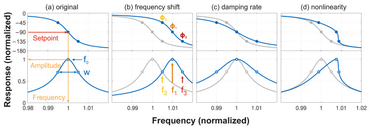 Figure 1
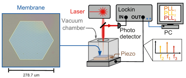 Figure 2
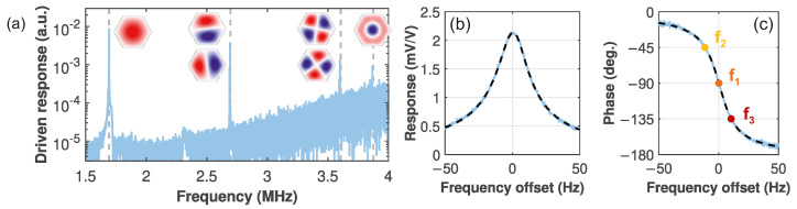 Figure 3
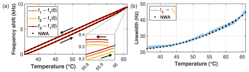 Figure 4
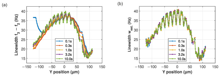 Figure 5
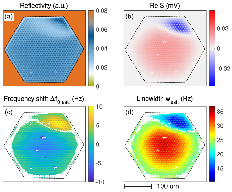 Figure 6
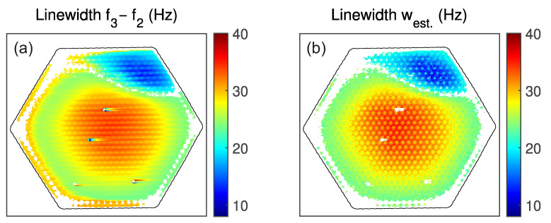 Figure 7
 Figure 8
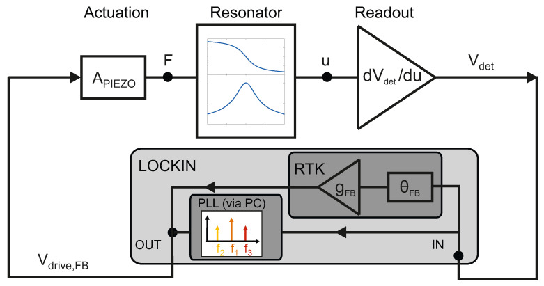 Figure 9
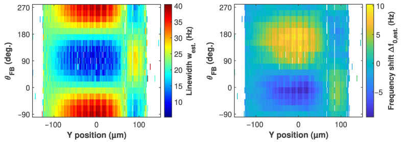 Figure 10
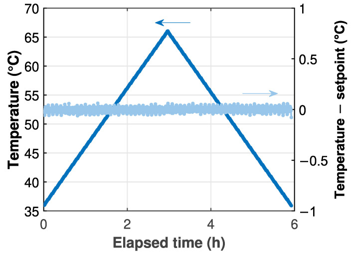 Figure 11
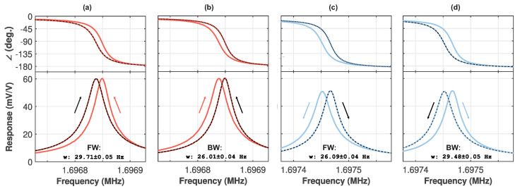 Figure 12
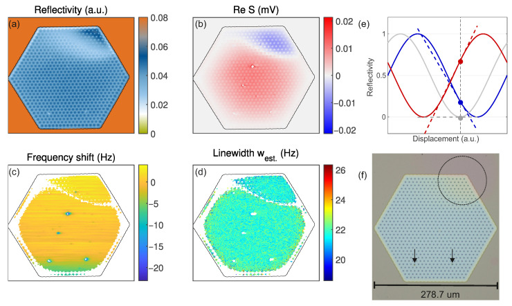 Figure 13
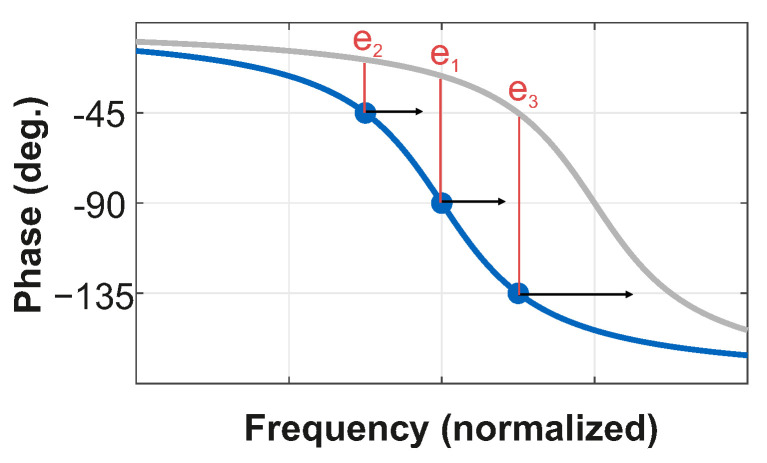 Figure 14
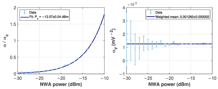 Figure 15
- —German Research Foundation (DFG)
- —TUM-IAS
- —German Excellence Initiative and the European Union Seventh Framework Programme
Peer Reviews
No public reviews on file for this paper yet. If you reviewed it on a platform where reviews are public (OpenReview, ICLR, NeurIPS, ICML), you can paste yours below so the community can read it here.
Videos
No videos yet. Explain this paper in a talk, walkthrough, or lecture? Add one.
Taxonomy
TopicsMechanical and Optical Resonators · Nonlocal and gradient elasticity in micro/nano structures · Advanced MEMS and NEMS Technologies
1. Introduction
Micromechanical systems have become a vital component of various technologies, including sensing. This ranges from gas detection to quantum applications [1,2,3,4,5], and communication systems [6], biomedical instrumentation [7], even to applications such as cancer diagnosis [8]. The performance and reliability of these devices are strongly influenced by their dynamic characteristics, particularly the frequency response, which determines key parameters such as resonance frequency, damping rate, and nonlinearities. Precise frequency-response characterization is therefore essential for monitoring these, but also for the understanding systems’ dynamics and ensuring stable operation under varying conditions. Traditional approaches—like recording linewidth maps of 2D material resonators [9], monitoring magnetic and electronic phase transitions [10] or optimizing a fabrication process, e.g., the influence of annealing on the quality factor [11,12,13]—to characterize mechanical resonators, typically involve sweeping the frequency of the driving force over the resonance to measure the amplitude and phase response. While effective, frequency sweeps are time-consuming and prone to drift over time, which limits their ability to track rapid changes. To overcome these limitations, frequency tracking can be achieved through phase-locked loops (PLLs). This has, e.g., enabled continuous monitoring of resonance frequencies with high precision [5,14,15,16]. Similar to the multi-frequency AFM technique, where either the first two modes [17,18] or higher harmonics [19] are used, our technique also uses several frequencies to gain information about resonators.
Here, we present a method for efficiently mapping and simultaneously tracking multiple properties—specifically, linewidth, frequency, and nonlinearity—of a mechanical resonator. We select three closely spaced frequencies within the width of a resonance peak, then follow them with PLLs and determine the desired quantities from the PLL outputs. First, we cover the concept behind our technique and then present the experimental realization in a micromechanical membrane. We start by tracking the resonators’ properties locally during a temperature sweep, then extend to spatially mapping them. Lastly, the nonlinear regime will be explored.
2. Concept
For tracking properties of a resonator, phase-locked loops (PLLs) are instrumental [14,20,21]. A PLL is locked to its setpoint as upon changes in phase, the frequency is adjusted accordingly, as illustrated in Figure 1a. The information can be in the frequency and/or in the amplitude. For example, we used the latter to record mode maps with high resolution, while remaining stable against external influences [22,23]. There, we chose one frequency per mode to map up to six modes of a membrane simultaneously, but here we use three frequencies within the peak of a single mode, see Figure 1. By choosing three setpoints —indicated by the filled symbols—instead of one per mode, we gain access to properties beyond amplitude and resonance frequency. These are traditionally obtained by taking frequency scans with a network analyzer (NWA) [24], which can be very time consuming.
As we will show in this section, with well-chosen setpoints, not only the frequency shift, but also the damping rate, and even the nonlinearity of the system can be determined straightforwardly. Traditionally, a setpoint of , corresponding to the maximum amplitude, tracks the resonance frequency (Figure 1a). Here, we use two additional PLLs. For a shift in resonance frequency , all three frequencies move in unison as depicted in Figure 1b. The frequency shift can thus be determined directly from . Figure 1c shows an increase in damping. Now, the center frequency remains unchanged, whereas and move apart symmetrically. In addition to the usual setpoint of , we select the two setpoints and strategically, so that directly yields the second parameter, the linewidth w, as we will see now. When driving our resonator at low powers, it behaves as a linear harmonic oscillator. The amplitude is given by the magnitude of the frequency response function , whereas its phase quantifies the delay between the drive and resulting motion. For simplicity, we focus on the case where the linewidth w is much smaller than the natural frequency and so that we can apply the Lorentzian approximation.
Note that, , where is the damping rate. Further, m is the mass of the resonator. The phase under the Lorentzian approximation is given by the following:
As the PLL phase and frequency are the measured quantities in our experiment, we want to utilize them to determine the linewidth and frequency. Rearranging the equation to calculate the linewidth w gives the following:
or
Choosing three setpoints also gives access to three phases, which we can use to determine our resonators’ properties. Specifically, for , . For , and for , so that and .
Still, with three frequencies, an additional property can be determined. Panel (d) shows that for increasing nonlinearity—as quantified by the Duffing parameter [25]—the phase of the response steepens on one side and flattens on the other. Thus, the equality between and no longer persists; this can be used to determine . However, operation in the nonlinear regime is potentially more complex than this simple picture, as we will see later. In the following, we first focus on the experimental realization in the linear regime and then return to investigate the nonlinearity.
3. Results and Discussion
The resonator we use to demonstrate our technique is a hexagonal micromechanical membrane made from high-stress silicon nitride (SiN) [26], as further described in the Methods Section (Appendix A). The sample is mounted on a piezo and excited with a lock-in amplifier, as shown in Figure 2. This particular membrane has a number of (unintentional) features, like thickness variations or particles on the devices, that are instrumental in showing the applicability of our technique in real-life situations, as discussed below.
Figure 3a shows the driven response of the membrane in vacuum. The different drum modes are visible and the insets show the simulated mode shapes of the first six modes. In the following, we focus on the fundamental mode near . The zooms [(b),(c)] display an exemplary resonance that is fitted well by a harmonic oscillator response [Equation (1)] (dashed), yielding a linewidth of .
3.1. Frequency and Linewidth Tracking During Temperature Sweep
The first demonstration of our technique is the tracking of the resonator’s properties during a large temperature ramp. The temperature was swept up and down from 36 to 66 °C over the course of six hours with the PLLs tracking the changes. Figure 4a shows the frequency shifts and (b) the linewidth as a function of temperature. NWA calibrations were taken at fixed intervals (black dots), and these match the results from our PLL well. Overall, the resonance frequency shifts up by : The substrate expands more than the membrane, resulting in a higher resonance frequency. The frequency shift shows hysteretic behavior as the temperature of the sample mount changes, but the chip temperature lags behind. This is also the cause for the offset, visible in the inset: The last point of the upward sweep is recorded, and an NWA measurement is done (≈ ). During this time, the setpoint temperature already drops, but that of the chip still rises. Hence, afterwards the first point of the downward measurement starts at a slightly lower temperature but higher frequency.
The corresponding linewidth in Figure 4b has more than doubled. This is due to increased coupling between the membrane and substrate modes [27]. The determined values again nicely match the NWA measurements, but extracting the linewidth precisely from the NWA traces requires some tricks in the data processing. These and other technical details can be found in Appendix B. Still, the measurement time is far longer than for the PLL technique.
A closer look at the inset in Figure 4a reveals something unexpected: there is an asymmetry in the frequency differences. This is because the PLLs need time to follow rapid changes. The asymmetry of and with respect to arises due to the dependence of the PLL response on the shape of the phase response. This results in a different lag for the different setpoints for a continuous frequency shift. This effect is explained in more detail Appendix D. To compensate for this, we use an estimator in the post-processing of the data, taking into account the tracking error of the PLL. The three phases and corresponding frequencies form a linear system of equations that can be solved, giving more accurate estimations for and w as demonstrated in the next Section.
3.2. Estimator
Up to now, there has been no distinction between the setpoint of the PLL and the actual phase. From the experiment, we know the measured phase consists of the PLL setpoint and its error :
The errors contain both a contribution due to the offset between the current frequency and the ideal one, as well as noise. The latter can be controlled via the bandwidth of the lock-in demodulator. The former may originate from, e.g., the lag of the PLL, but can be compensated for, as we will show now. With the three phases , we can set up a linear equation system based on Equation (4), allowing us to determine the estimated linewidth and frequency . This system of three linear equations and two unknowns is solved (as the least squares solution) by Matlab’s -operator:
The result contains the estimated frequency and linewidth . Note that, absent noise, Equation (6) gives the exact values independently of the PLLs being at their setpoints. Readout noise mainly affects , resulting in deviations in the estimated parameters. The exact effect depends on the setpoints and PLL operations, but, in general, the more noise, the larger the deviations will be. As two parameters are sufficient to determine frequency and linewidth, the third can be used to determine an additional property, or simply for a consistency check.
To demonstrate the benefits of using the estimator, we compare both methods of extracting the linewidth in Figure 5. There, although the spatial dependence will be covered in detail in the next section, we already step over the membrane, recording the three PLLs for different waiting times between movements. Throughout the trace, sharp features from the membrane holes appear, which the PLL has to follow. If the waiting time is long enough, it will be able to adjust and . However, for short waiting times, shows a long distance before settling, and no sharp features are seen. Increasing the wait to 10 s per point sharpens the features in the line trace, but recording a correct map would require long measurement times. Also, the ability to track rapid changes is lost when the PLL needs 10 s per point to follow the changes. The short waits are also shifted to the right, indicating a delay between the changing linewidth and the reaction of the PLL. In contrast, with , all traces coincide and show the sharp features, even for the shortest wait of 0.1 s. The estimator thus enables high-resolution mapping and tracking with short measurement times.
3.3. Mapping of Resonator Properties
From measuring at one position on the membrane, we extend to full spatial mapping of its properties. However, as neither systematic frequency shift nor linewidth change with position is expected in our membrane, we introduce these by implementing a feedback loop that feeds the measured displacement back with a controllable gain and phase shift [28,29] as detailed in Appendix A. A feedback force that is in phase with the displacement shifts the frequency, whereas feedback that is in phase with the velocity alters the damping, i.e., the linewidth w [30]. Since the total loop gain depends on , as well as on the open-loop response (varying on the micrometer scale due to the release holes and slower due to the mode shape and readout), this results in both fine and large-scale features in the local frequency shift and damping rate.
Figure 6 shows the spatial map of various properties in the presence of feedback: (a) shows the reflectivity and (b) the amplitude of PLL 1. The latter deviates from the expected mode shape [Figure 3a], as the membrane has a region with a different SiN thickness where the sign of the readout is reversed. This is explained in more detail in Appendix C Figure A5 [31]. Figure 6c shows the frequency shift; (d) the estimated linewidth. White spots in any of the maps indicate contamination on the membrane where the laser locally heats the membrane, shifting down sharply and reducing the signal. These points are either excluded due to low signal or large errors . Yet, the PLL tracking remains robust to such real-world features, including sign reversal.
In the center of the membrane, the frequency shifts downward relative to the edge, and in the upper-right corner it shifts upward as the loop gain switches sign. Overall, a very fine structure is visible, and even the holes in the membrane can be resolved. A similar pattern occurs in the linewidth (d). There, the linewidth increases at the center of the membrane and decreases in the upper-right corner, again due to the applied feedback. Without it, the linewidth is constant at ≈22 Hz on the whole membrane, as shown in Figure A5. There, the same measurement without feedback is shown.
Also, for the maps, the estimator is applied during data post-processing, highlighting the methods’ benefits. Figure 7 compares the maps of the linewidth in the presence of feedback using the two methods on the same data. Both maps show similar magnitudes and trends, with the largest damping in the center and the smallest in the upper right corner. The map of , also shows a larger linewidth at the lower and right edges. This is, however, because the PLLs need time to settle into the correct frequencies, and the errors are still large. Although the holes are visible, the picture appears rather blurred. In contrast, the map generated using the estimator shows much finer features and does not exhibit artifacts such as unexpected high linewidths at the edges or at the spots where particles are located. Further only needs a short time to settle after the particles, unlike , where streaks are visible on the right side of the particles.
As each point only takes ≲ (mainly limited by stage motion), mapping such fine structures in w and can be done much faster with our three-tone PLL than by recording a whole NWA trace for every single point over the whole membrane [22,32], which would take weeks to complete.
3.4. Operation in the Nonlinear Regime
The final property that can be determined with our technique is the nonlinearity. Thus far, the membrane has been driven in the linear regime; increasing the driving allows access to the nonlinear response. In Figure 8a the driven response for different driving powers with only one tone (“pump”) is shown. When the drive increases, the resonance takes the shape of a Duffing response. Although the amplitude is affected by nonlinear readout, the phase—used by the PLLs—is not [26]. Its slope gets steeper with increasing excitation power, as was shown in Figure 1d so an asymmetry between and could be expected. Unfortunately, the nonlinearity makes the situation more complex: to apply our technique, we require three driving tones, but already adding a second, strong tone gives rise to very complex effects [33,34]. Hence, instead of equally strong tones for all PLLs, we use weak probes [35]. Figure 8b shows the responses of one probe for varying pump powers. Starting with a single relatively weak pump tone ( ) at a fixed frequency, the probe response is only slightly shifted compared to the case with no pump (gray). This one, in turn, closely matches the original linear response. Increasing the pump power leads to more complex probe responses. This is still captured by an analytical expression [36], which also shows that adding another weak probe can be done independently, see Figure A5. For frequencies higher than the pump, the measured amplitude and phase in Figure 8b look like a shifted linear response; the stronger the pump, the larger the shift. For lower frequencies, the response becomes more complex, with the phase developing a peak with positive values. Figure 8c shows a color plot of the calculated probe response phase versus nonlinearity induced by a -locked strong pump. Note that PLLs would follow the contour lines. Like the traces in (b), all setpoints shift towards higher frequencies. The pump at is indicated in blue; the line remains on the right side of the pump, hence we keep that setpoint for . However, the previous would cross the pump relatively quickly as the pump power increases. Hence, in the presence of small nonlinearities, PLL 2’s lock would already be lost since the frequencies approach each other. Therefore, a different setpoint has to be chosen. Indicated in Figure 8c are and . The trend of the former is no longer monotonic and would therefore lead to loss of PLL lock when increasing or decreasing pump power. Contrarily, the setpoint is farther from the pump than , while still being monotonous, and can therefore track higher pump powers.
The measurement with the adjusted values is shown in Figure 8d. The black lines indicate the scaled lines from (c). The different colors represent measured data points that match the theoretical curves well. In the linear regime, for small pump powers, the PLL frequencies evolve in unison. When increasing the pump, they shift upward as the response enters the Duffing regime. Above , a rather sharp transition is reached. There, the setpoint approaches the pump frequency but still matches the calculations. In the experiment, there is a limit on how close two frequencies can get. More importantly, from the scaling of the contour lines, not only and are obtained, but also the amount of nonlinearity. Specifically, we find a critical pump power of . This matches well with the value of that was determined independently from driven responses acquired at different network analyzer powers as discussed in Appendix E. Hence, not only the linear properties but also the nonlinearity of the strongly driven resonator can be determined using our method.
3.5. Discussion
In this final section, we discuss further possibilities of applying and extending the presented method. Until now, we demonstrated single-mode operation. The method can easily be extended to track two modes, as the lock-in we use has six demodulators. This is not a fundamental limitation; with a different measurement device, the number of modes can be increased even further. In general, the operation relies on the steadiness of the phase response. For modes that remain far in frequency, this is usually not an issue. Also, as long as does not change, our method will also work for densely spaced modes. Only when nearly degenerate modes begin to interact does the phase response change, preventing reliable operation.
Currently, the available frequency range is limited by the piezo actuator. It has a resonance frequency of , after which the amplitude decreases. To expand the available range, one could switch to an electrostatic or an optical actuation scheme. Ultimately, the measurement is limited by the signal coming from the resonator, as the phase must be reliable enough to lock to. Further, there are different ways to implement the PLLs. One could, e.g., use dedicated hardware, enabling a faster operation and more deterministic timing. Specifically, using the real-time kit of the lock-in to implement the PLLs is a possibility to track sub-second changes with the current setup.
Finally, we emphasize that our technique is not limited to optomechanical readout of micromechanical membranes and can be applied to various systems. It is generic, i.e., independent of the optical readout and piezo actuation used in our case. The requirements for our method are solely the ability to perform a PLL measurement and a sufficient signal-to-noise ratio, so that the phase remains stable enough to remain locked throughout the measurement. We believe that the method can be straightforwardly applied to a wide variety of resonators, including, e.g., MEMS with capacitive readout and electrostatic actuation.
4. Conclusions
In conclusion, we demonstrate a fast and efficient method for tracking and mapping properties of a mechanical resonator, such as frequency shift, linewidth, and nonlinearity, using three strategically chosen driving frequencies instead of repeatedly recording frequency sweeps. This robust method allows us to investigate a range of unintentional features of our resonator, such as thickness variations, particles on the membrane, and temperature-dependent linewidth. Thus, it enables rapid characterization, spatial mapping, and real-time monitoring of the properties of changing systems.
The reference list from the paper itself. Each links out to its DOI / PubMed record.
- 1Sanz-Jiménez A. Malvar O. Ruz J.J. García-López S. Kosaka P.M. Gil-Santos E. CanoÁ. Papanastasiou D. Kounadis D. Mingorance J. High-throughput determination of dry mass of single bacterial cells by ultrathin membrane resonators Commun. Biol.20225122710.1038/s 42003-022-04147-536369276 PMC 9651879 · doi ↗ · pubmed ↗
- 2Sader J.E. Hanay M.S. Neumann A.P. Roukes M.L. Mass spectrometry using nanomechanical systems: Beyond the point-mass approximation Nano Lett.2018181608161410.1021/acs.nanolett.7b 0430129369636 · doi ↗ · pubmed ↗
- 3Bhattacharya G. Lionadi I. Mc Michael S. Taverne M. Mc Laughlin J. Fernandez-Ibanez P. Huang C.C. Ho Y.L.D. Payam A.F. Two Dimensional-Material-Coated Microcantilevers for Enhanced Mass Sensing and Material Characterization Nanoscale 202517272002721510.1039/D 5NR 03147 H 41235413 · doi ↗ · pubmed ↗
- 4Li T. Zhao P. Wang P. Krishnaiah K.V. Jin W. Zhang A.P. Miniature optical fiber photoacoustic spectroscopy gas sensor based on a 3D micro-printed planar-spiral spring optomechanical resonator Photoacoustics 20244010065710.1016/j.pacs.2024.10065739525924 PMC 11550629 · doi ↗ · pubmed ↗
- 5Bleszynski-Jayich A.C. Shanks W.E. Peaudecerf B. Ginossar E. von Oppen F. Glazman L. Harris J.G.E. Persistent Currents in Normal Metal Rings Science 200932627227510.1126/science.117813919815772 · doi ↗ · pubmed ↗
- 6Bozkurt A.B. Golami O. Yu Y. Tian H. Mirhosseini M. A mechanical quantum memory for microwave photons Nat. Phys.2025211469147410.1038/s 41567-025-02975-w · doi ↗
- 7Arlett J. Myers E. Roukes M. Comparative advantages of mechanical biosensors Nat. Nanotechnol.2011620321510.1038/nnano.2011.4421441911 PMC 3839312 · doi ↗ · pubmed ↗
- 8Kosaka P.M. Pini V. Ruz J.J. Da Silva R. González M. Ramos D. Calleja M. Tamayo J. Detection of cancer biomarkers in serum using a hybrid mechanical and optoplasmonic nanosensor Nat. Nanotechnol.201491047105310.1038/nnano.2014.25025362477 · doi ↗ · pubmed ↗