Biological Functional Class Enrichment Analysis with R, an Annotated Tutorial for Bench Scientists
Kejin Hu

TL;DR
This paper provides an accessible R tutorial for bench scientists to perform biological functional class enrichment analysis using tools like GO, KEGG, and Reactome.
Contribution
The paper introduces an annotated R tutorial with detailed scripts for FunCEA, tailored for biomedical researchers with minimal computational expertise.
Findings
The tutorial covers two popular FunCEA methods: over-representation analysis and functional class scoring.
It provides annotated R code for visualizations such as dot plots, term-gene network plots, and GSEA plots.
The tutorial uses freely available R packages and databases, eliminating the need for commercial software.
Abstract
High-throughput sequencing generally results in a list of genes. Which functional groups of genes among the DEGs are meaningful underlying factors to the differential biological/biomedical conditions under investigation? The process to find answers to this question can be called biological functional class enrichment analysis (FunCEA). R is a robust platform for FunCEA due to its accessibility by general users and availability of well-developed R packages for enrichment analysis and visualization, as well as for knowledge databases. Bench scientists in biomedical sciences need accessible and easy-to-understand protocols for FunCEA. This R tutorial provides detailed R scripts or command lines for FunCEA, as well as for data processing and visualization of the enrichment results. It keeps bench scientists in mind and provides supportive and apprehensible descriptions of the R scripts for…
Genes, proteins, chemicals, diseases, species, mutations and cell lines named across the full text — each resolved to its canonical identifier and authoritative record.
Click any figure to enlarge with its caption.
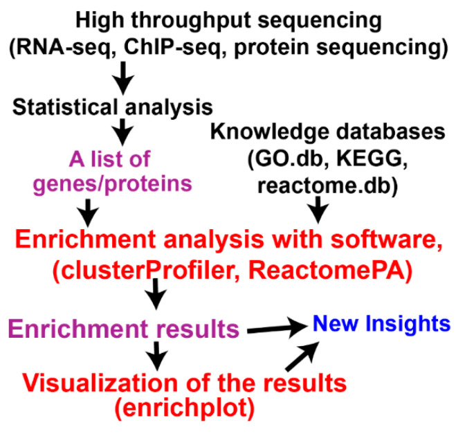 Figure 1
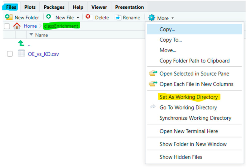 Figure 2
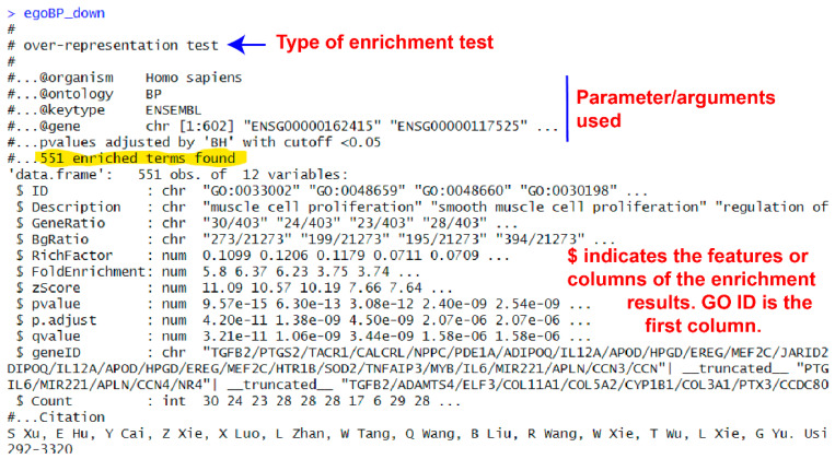 Figure 3
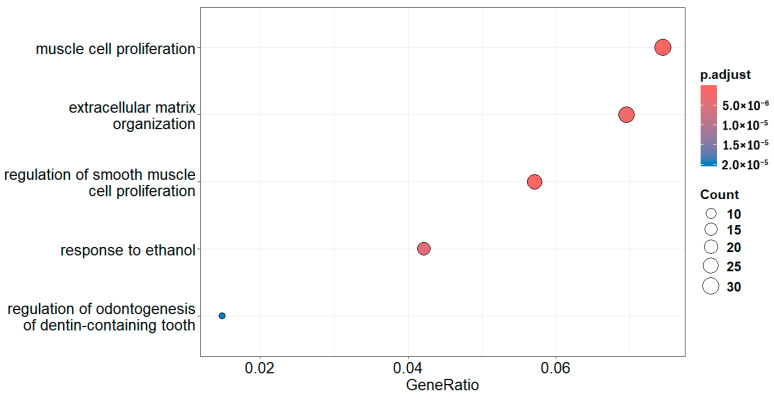 Figure 4
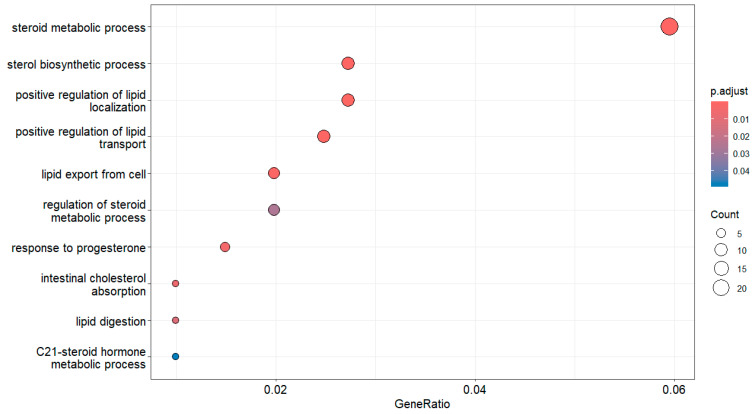 Figure 5
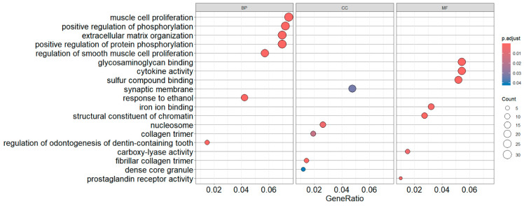 Figure 6
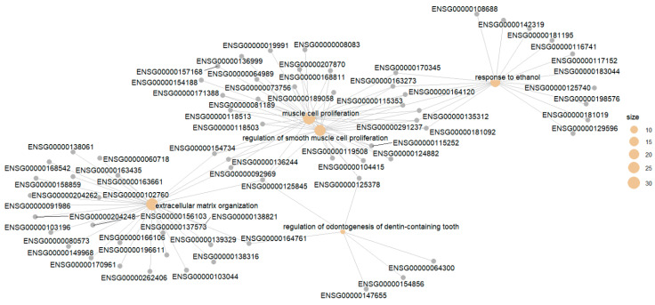 Figure 7
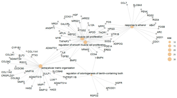 Figure 8
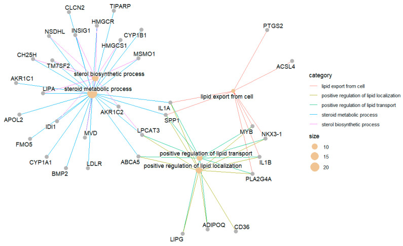 Figure 9
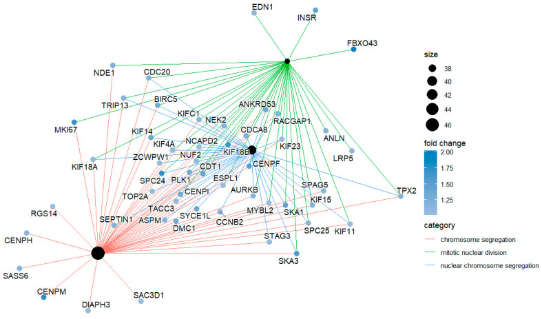 Figure 10
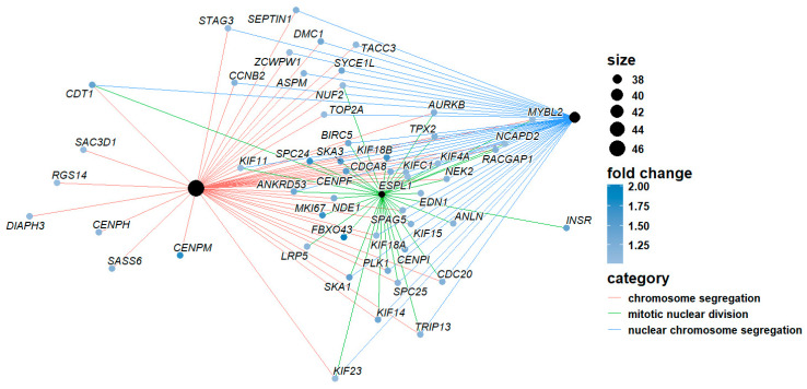 Figure 11
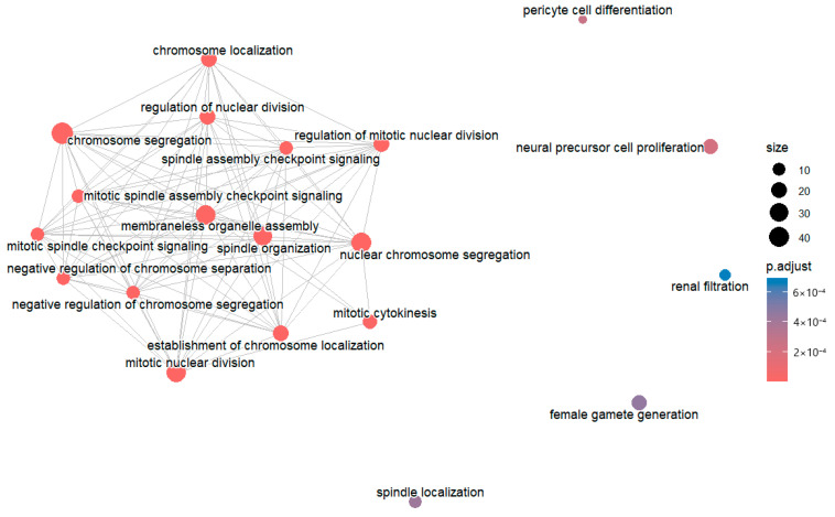 Figure 12
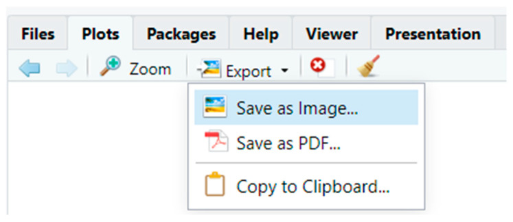 Figure 13
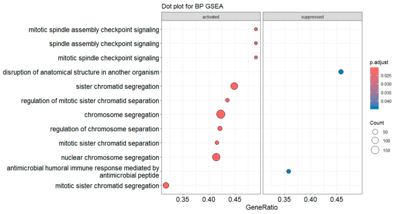 Figure 14
 Figure 15
 Figure 16
 Figure 17
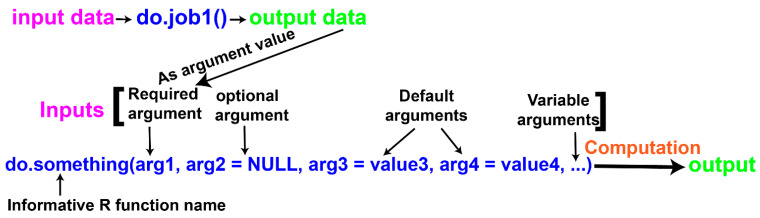 Figure 18
 Figure 19
- —UNT
Peer Reviews
No public reviews on file for this paper yet. If you reviewed it on a platform where reviews are public (OpenReview, ICLR, NeurIPS, ICML), you can paste yours below so the community can read it here.
Videos
No videos yet. Explain this paper in a talk, walkthrough, or lecture? Add one.
Taxonomy
TopicsBioinformatics and Genomic Networks · Gene expression and cancer classification · Genetic Associations and Epidemiology
1. Introduction
High-throughput sequencing (HTS) is a commonplace approach in biological and biomedical sciences. HTS generally results in a list of genes/proteins that significantly differ between two conditions (Figure 1), which constitutes the secondary data in question. Accurate characterization of the resulting gene list is the essential part of HTS experiments. The list could include hundreds to thousands of genes. Functional characterization of that many genes is challenging, and designated software programs are needed to achieve efficient, quick, and accurate profiling of genes in the list. This process can be generally called biological functional class enrichment analysis (FunCEA for easy pronunciation). FunCEA tests whether each set of genes in the same functional group is significantly overrepresented in the resulting experimental gene list. FunCEA currently employs three different algorithms: over-representation analysis (ORA) [1], functional class scoring (FCS) [2], and pathway topology (PT) [3]. To functionally profile a list of experimental gene products, FunCEA requires gene function knowledge databases. There are many gene function knowledge databases, and this tutorial uses gene ontology (GO) annotation database (GO.db) [4], Kyoto Encyclopedia of Genes and Genomes (KEGG) [5], and reactome pathway database [6]. There are many R software packages for this purpose as well, and this tutorial introduces clusterProfiler [7,8] and ReactomePA [9]. The clusterProfiler package is used because it integrates two of the three approaches currently available, i.e., ORA and FCS. It also has several companion packages including enrichplot [10] and ReactomePA. Those R packages are widely used and well-maintained by the Yu group [7,11]. Visualization of enrichment results is critical in understanding and communication of the enrichment results. The enrichplot R package provides many functions to graphically summarize the enrichment results. The enrichplot package is based on the popular ggplot2 graphics package, which can enhance the enrichment result visualization.
There are some web-based tools for FunCEA such as PANTHER (https://archive.pantherdb.org/, accessed on 17 January 2026) and DAVID (https://davidbioinformatics.nih.gov/, accessed on 17 January 2026), but the R-based methods using designated packages are more robust, versatile, and professional. Figure 1 depicts the FunCEA workflow. We will focus on ORA and FCS using the annotation databases GO.db, KEGG, and reactome.db. In addition to enrichment analysis, this tutorial also describes various R functions for visualization of the enrichment results. For easy reading and practicing, all executable R codes/commands start in a separate line with an indent and are highlighted in red text. Those red codes are intended to be typed in RStudio Console pane and practiced by the readers. Following R convention, comments on codes/scripts are indicated with a leading pound sign # immediately after the corresponding codes. R functions, operators, and arguments mentioned in the text part (not the code part) are highlighted in italicized blue text. R package names and other R terms are italicized only.
This tutorial is designed in a way that bench scientists with no experience in R programming can follow. The audience can learn both FunCEA and R skills by practicing this tutorial. I thus try to use plain language and provide detailed annotations to the R codes, especially when a new R term or concept first appears. Those who have no prior R experience may be more comfortable to learn the introduced skills here after they quickly learn one or both R-related tutorials from the same author [12,13]. I always believe that the most efficient learning is achieved by doing. It is thus advised that the audience type the provided codes and review the code outputs in RStudio, rather than just reading the code texts. I will include some code output as screenshots or figures, but most of the time readers should check the code outputs/results on R screens of different panes (i.e., panes of Console, Plots, Environment, and Data Viewer). The key to conducting FunCEA in R is a good understanding and proficient use of R functions and other basic R concepts. For this purpose, this tutorial includes Appendix A to introduce the basics of R functions, data frames, vectors, and objects. Finally, an R Markdown file with codes for the major steps and its rendered HTML version are included as Supplementary Materials of this tutorial. The HTML output file include codes output and plots, which help the audiences better understand FunCEA.
2. Materials and Equipment
2.1. Equipment
A desktop or laptop computer (either PC or Mac). Internet access is needed since clusterProfiler directly interrogates the KEGG knowledgebase via internet. Internet connection is also essential to install R, RStudio, and the relevant R packages.
2.2. Sample Data
RNA-seq statistical result in comma separated values (CSV) format is used as the starting data. Starting with this real-world data rather than a pre-prepared gene list from a package benefits beginners. It is available as the Supplementary Materials with a file name of OE_vs_KO.csv.
2.3. Software
No commercial software is needed. This tutorial uses R (V4.5), RStudio (2025.5.0.496), and the relevant R external packages (clusterProfiler, org.Hs.eg.db, enrichplot, AnnotationDbi, ggplot2, dplyr, ReactomePA, GO.db, ggtangle, and others). All are open source and free to use. The versions of major packages used in this tutorial were clusterProfiler (V4.16), org.Hs.eg.db (V3.21), ReactomePA (V1.52), GO.db (V3.21), enrichplot (V1.28.4), and AnnotationDbi (V1.70).
3. Raw Data and Its Import to R
Before analysis, install R (https://www.r-project.org/) and RStudio (https://posit.co/download/rstudio-desktop/). Make sure you install R before RStudio. If you encounter any issues installing R or RStudio, please consult your IT support team or any knowledgeable and supportive person.
We use results of RNA sequencing (RNA-seq) as an example for biological FunCEA of a gene list (see Supplementary Data). The file name of the DESeq2 [14] output is OE_vs_KO.csv. This RNA-seq project studied the role of human BRD2 in induced pluripotent stem cell (iPSC) reprogramming in the author’s lab [15]. We compared the transcriptional differences between BRD2 overexpression (OE) and knockout (KO) in human fibroblasts that undergo iPSC reprogramming. You can create a new folder of classEnrichment and save OE_vs_KO.csv in the classEnrichment folder (directory in R terminology). Set this folder as the working directory (WD) using the base R setwd() (stands for “set working directory”) function (see Appendix A.1 for a description of R functions) in the RStudio Console pane (the lower-left pane as its default location). Type the following code in the Console pane and then hit the Enter key (like this code, you should hit the Enter key to execute all other codes in red text in this tutorial, which is not explicitly stated in all the codes),
setwd(“full_path2classEnrichment”) # Set the folder where the OE_vs_KO.csv file is located as the R working directory. You need to use your full path, which is different from the path description I wrote here.
Alternatively, in the Files pane (the lower-right pane as its default location in RStudio), navigate to the classEnrichment folder, and then click on “More” cog tab in the tab bar of the Files pane to bring about the pulldown menu (Figure 2). Click “Set As Working Directory” on the pulldown menu. On the Console pane, you can see the corresponding full command line for the same action.
After setting up the working directory, you can see the full path to your working directory by executing,
getwd() # This function means “get working directory”. The full path will be printed out in the Console pane.
Upon setting the folder with your file as the working directory, you can list and see the files using the list.files() function. Just run,
list.files() # This command prints out the files in the current working directory onto the Console screen.
Read in the RNA-seq results data into R using the base R function read.csv() and put the data in an R object named rawData (see Appendix A.4 for a brief introduction to R objects). To bring about the built-in help page of read.csv(), type and run ?read.csv or execute help(read.csv) in the RStudio Console. The help page will show in the Help pane. For other functions in this tutorial, you can find the help pages using ? or help() function as you do for read.csv() here.
rawData <- read.csv(“OE_vs_KO.csv”) # The rawData object will show on the Environment pane in the upper-right quadrant (refer to Appendix A.4 for R objects). The file name should be quoted. This code reads the file into R from the working directory. You can read in a file from any other directory when the full path to the file is included.
The rawData here looks like a common table but is a data frame in R terminology, which is a two-dimensional data structure like an R matrix (see Appendix A.2 for a description of data frames and matrices). You can test whether an R object is a data frame with the R test function is.data.frame(),
is.data.frame(rawData) # This command should return TRUE, an R logical value.
Review the data in the Data Viewer pane (upper-left pane by default) by executing,
View(rawData) # This can also be achieved by clicking the rawData object on the Environment pane.
dim(rawData) # It reveals the number of rows and columns using the dimension function dim(). As shown, the data frame contains 35,953 rows and 14 columns.
In the Data Viewer pane (in the upper-left quadrant by default), you can scroll down and up, left and right to review the data. You can also sort the data based on any column by clicking the column name.
Or, you can know the entire table structure by printing out the first 2 rows with the column names,
head(rawData, n = 2)
4. Install R Packages for Functional Class Enrichment Analysis
The functions used in Section 3 above are from R base packages. We need several external R packages to conduct FunCEA. An R package is a standardized collection of R codes, functions, sample data, built-in documentation (e.g., help pages and user manual, i.e., vignette in R terminology), or a compilation of knowledge with associated methods. The R core team develops the R base packages, but most R packages are user-developed external ones, which extend R functionality. There are two groups of external R packages for FunCEA: software or tool packages for analysis or visualization, and knowledgebase packages. Knowledgebases for this tutorial include org.Hs.eg.db, reactome.db, and GO.db. The package clusterProfiler can interrogate the KEGG web database directly using its built-in functions like bitr(), bitr_kegg(), and search_kegg_organism(). This way, you use the mostly updated KEGG knowledge database and no KEGG annotation package is needed in R. The software/tool packages include clusterProfiler, enrichplot, and ReactomePA. The clusterProfiler package provides many functions for FunCEA while enrichplot includes many functions for enrichment visualization. Those packages are deposited in the Bioconductor repository. When you install ReactomePA, reactome.db is automatically installed. The GO.db package is required for GO enrichment analysis, but one does not need to explicitly load it.
We use the BiocManager::install() function from the BiocManager package to install packages from the Bioconductor repository. However, the BiocManager package itself is installed using the base R package installation function of install.packages(). If BiocManager package is not installed, you need to install this tool first,
install.packages(“BiocManager”) # You will see BiocManager is now added in your Packages pane.
BiocManager::install(version = “3.22”) # You can see now the biocVersion package in the Packages pane after this command. The version may not be 3.22 at the time you install it; 3.22 is the version when this tutorial was written. Make sure your BiocManager version matches the R version.
Next, we install the annotation tool package AnnotationDbi from the Bioconductor repository,
BiocManager::install(“AnnotationDbi”) # When you install AnnotationDbi, a lot of dependencies/imports packages are automatically installed, including the following core dependencies: BiocGenerics, Biobase, S4Vectors, IRanges, and RSQLite.
The following codes represent formats for installing packages from Bioconductor. The first line tests whether BiocManager is installed or not using the if() statement. The require() function within if() acts similarly to library(). When !require(“BiocManager, quietly = TRUE) returns a TRUE, which means BiocManager is not installed, the second line installs the BiocManager package. Otherwise, i.e., a FALSE is returned by !require(“BiocManager, quietly = TRUE), the second line is skipped. The remaining lines install each Bioconductor package using the BiocManager::install() function.
if (!require(“BiocManager”, quietly = TRUE)) # This script tests whether BiocManager is installed or not. The exclamation mark “!” here is a logical “not” operator, which means “negate”. Run !require(“BiocManager, quietly = TRUE) to see its return/result.
install.packages(“BiocManager”) # It installs BiocManager if it is not installed as tested in the first line.
BiocManager::install(“clusterProfiler”) # This installs clusterProfiler from Bioconductor repository.
BiocManager::install(“enrichplot”) # This installs enrichplot from Bioconductor repository.
BiocManager::install(c(“ReactomePA”, “org.Hs.eg.db”, “GO.db”)) # Multiple packages can be installed with one R script when you put them in a vector as shown here for packages of ReactomePA, org.Hs.eg.db, and GO.db. The base R c() function generates an R vector (see Appendix A.3).
5. ORA for GO Enrichment Analysis
5.1. Preparation of Gene Lists for ORA Analysis
For ORA enrichment analysis, we focus on the genes that are differentially expressed. ORA input gene lists include two types: one is the up-regulated and the other is the down-regulated. We usually analyze the two lists separately. ORA analysis just needs the gene IDs in an R vector (a gene list in plain language) as input. R vectors are one-dimensional structure of the same type of data (see Appendix A.3). The gene list may and may not be ranked, and a bare list of genes without the associated expression values works.
First, subset the up-regulated data using the base R subset() function,
sigUpData <- subset(rawData, subset = log2FoldChange > 1 & padj < 0.05)
The above script subsets genes that are significantly up-regulated by at least 2-fold at the significant level of padj < 0.05. It uses two criteria to subset the data with the logical operator & as shown in this code. Those rows (genes, or transcripts) that meet both conditions are kept. This code keeps all columns. For details of subset() function, find its help page by issuing help(subset) or ?subset in RStudio Console pane. For a general introduction of R functions, see Appendix A.1. We store the resulting small data frame (less rows) in an R object sigUpData using the assignment operator <-. R objects are stored temporarily on your computer active memory that is available for subsequent use during your R session. Otherwise, the resulting small data frame is just printed out on your screen and cannot be used in the following analysis.
You can check the dimension of the resulting data frame,
dim(sigUpData) # The dimension function dim() reveals that there are 775 rows only now. The dimensional information is also displayed in the Environment pane.
Similarly, we can subset data for the down-regulated genes,
sigDownData <- subset(rawData, subset = log2FoldChange < −1 & padj < 0.05) # This code subsets genes that are significantly down-regulated by at least 2-fold at the significant level of padj < 0.05. The logical operator & is used in this code to define two criteria for subsetting.
The above code uses two conditions to subset: one is the log2FoldChange and the other is the padj values. It just uses the column name to define conditions for subsetting for the selected columns. When two criteria (two columns) are used to subset the data frame, you use the logical operator & to indicate that the two conditions must be met as shown above. Please note that the thresholds are arbitrary depending on your projects. In this protocol, we use 2-fold as the threshold, i.e., log2(fold change) > 1, or log2(fold change) < −1.
You can review sigUpData in the Data Viewer pane (upper-left) by clicking sigUpData in the Environment pane, or just issue,
View(sigUpData) # View the subsetted smaller data frame in the Data Viewer pane.
As you can see, the first column is ENSEMBL IDs. The ENSEMBL IDs in this column will be our input gene list for GO ORA. You can extract this gene list as follows,
sigUpGeneList <- sigUpDataENSEMBL # It uses the extraction operator ** along column name to extract one column of data from a data frame as a vector as demonstrated here.
Alternatively, you can generate the gene list using the square bracket extraction operator [ ] by either index (position of the column) or column name with a syntax of [row, column].
sigUpGeneList1 <- sigUpData[, 1] # Extract by index. ENSEMBL is column 1. The comma without a row number here indicates that all rows are extracted to the new data frame (multiple columns) or the resulting vector (when one column extracted). Because the drop argument defaults to TRUE, the resulting data are a vector. It will be one column data frame when its value is defined as FALSE, i.e., sigUpData[, 1, drop = FALSE].
sigUpGeneList2 <- sigUpData[, “ENSEMBL”] # Extract by column name, i.e., ENSEMBL.
The above three gene lists are identical, and those can be tested using the R test function identical(),
identical(sigUpGeneList, sigUpGeneList1) # The return is TRUE.
identical(sigUpGeneList, sigUpGeneList2) # The answer is TRUE.
Similarly, you can generate the list of genes down-regulated by BRD2,
sigDownGeneList <- sigDownData$ENSEMBL # Or, use sigDownData[, “ENSEMBL”]
5.2. Load the Required Packages
With the gene list generated, we can profile the genes for GO term enrichment using the function of enrichGO() from the clusterProfiler package. First, we need to load the tool package clusterProfiler using the library() function,
library(clusterProfiler) # You can also load any package by clicking the box on the left of the package name in the RStudio Packages pane.
To see the original literature of clusterProfiler, you use the citation() R function,
citation(“clusterProfiler”) # This command lists the original publications from Dr. Yu’s group.
To find out the package manual/vignettes,
browseVignettes(“clusterProfiler”) # It pops up a window containing the hyperlink for the package documentation in the default browser. Clicking the HTML will lead to the landing page that includes hyperlinks of different topics, including the vignette.
To conduct GO enrichment analysis, we also need the knowledgebase package. Only the organism-level annotation package needs to be loaded. GO.db should be installed, but may not be loaded. Since human genes are analyzed here, we load the org.Hs.eg.db package,
library(org.Hs.eg.db) # This also loads the basic AnnotationDbi and other required Bioconductor and annotation packages (Biobase, generics, BiocGenerics, IRanges, S4Vectors, and stats4). Other organisms have their own organism-level annotation packages; for example, you install and load org.Mm.eg.db if the genes in your input gene list are mouse ones.
5.3. Generate the Enrichment Object Using the enrichGO() Function
Gene ontology (GO) is commonly analyzed in FunCEA. GO has three sub-ontologies: biological process (BP), molecular function (MF), and cellular component (CC). clusterProfiler package provides functions to conduct GO enrichment analysis. The enrichGO() function conducts the traditional ORA of gene ontology.
The simplified syntax for enrichGO() with the first four arguments is as follows.
enrichGO(gene, OrgDb, keyType = “ENTREZID”, ont = “MF”) # This is not a code for practice. It is the syntax.
The full syntax can be found on the built-in help page, which can be pulled out by running,
help(enrichGO) # Or, simply execute ?enrichGO.
The above syntax includes four basic arguments (parameters in plain language). The first argument gene defines the list of input genes; OrgDb defines the organism-level annotation package; keyType defines the type of gene ID with ENTREZID as the default; and ont defines GO category, which could be BP, CC, MF, or ALL (MF as the default). The first and the second arguments (gene and OrgDb) have no default values. These arguments are called required arguments, for which users need to provide values. For an introduction of R function and its arguments, refer to Appendix A.1.
Let us analyze BP enrichment for the human gene list of sigDownGeneList,
egoBP_down <- enrichGO(gene = sigDownGeneList, OrgDb = org.Hs.eg.db, keyType = “ENSEMBL”, ont = “BP”) # The results are stored in egoBP_down object. Since our gene list uses ENSEMBL IDs, we change the keyType setting from the default “ENTREZID” to “ENSEMBL”. When you want to analyze biological process, you change the ont setting from the default “MF” to “BP”.
The argument names can be omitted if you position all of the values in the order shown in official syntax (function definition order). When the argument names are omitted, the order of the arguments is strictly enforced. When all of the argument names are provided, the order of arguments inside the parentheses of the function does not matter. The above code can be simplified as,
egoBP_down <- enrichGO(sigDownGeneList, org.Hs.eg.db, “ENSEMBL”, “BP”) # This simplified code works, but it would not work when the order of the argument values would be changed. Readers are encouraged to change the positions of the four argument values here and experience what happens.
5.4. Review and Extract the Enrichment Results as a Traditional Data Frame
The resulting enrichment object (egoBP_down) is an R S4 data structure, which is not immediately human-accessible or readable.
isS4(egoBP_down) # The isS4() function tests whether it is an S4 object.
You can have an overview of the results by simply issuing the object name,
egoBP_down # This is implicit use of print(egoBP_down).
The above code prints out an overview of the results. You can see information about the analysis; for example, type of analysis, argument values used, and summary of enrichment. In this example, it shows “551 enriched terms found” at the time of writing (the number of enriched terms may vary when the tutorial will be used due to update of knowledge databases). The enrichment statistics include 12 features that are present in 12 columns in the result data frame. When the contents are long for any item, only the first several items are printed out (see Figure 3).
The primary elements of an R S4 object (data structure) are slots. You can list the names of slots in an S4 object using the slotNames() function,
slotNames(egoBP_down)
You can see that there are 15 slots and the first one is result. We can access S4 object slots using the @ S4 accessor. Let us extract the enrichment analysis result slot,
egoBP_downRes <- egoBP_down@result # This extracts the enrichment statistics results as a data frame using the @ operator from the result slot.
View(egoBP_downRes) # The View() function allows you to review the results in the Data Viewer pane. You can just click eogBP_downRes in the Environment pane to bring its contents to the Data Viewer pane.
Now, the results in the resulting data frame are easy to read and understand. You can scroll up and down the table or left and right in the table to review. You can sort the values of any column by clicking the column name.
The resulting data frame (table in plain language) includes all results (enriched and non-enriched). If you just want to generate a data frame for the enriched terms, use the following code,
egoBP_downEnrichedRes <- as.data.frame(egoBP_down) # The as.data.frame() function extracts result for the enriched terms only as a data frame.
The results obtained by the above two methods (@ accessor or as.data.frame()) are both traditional data frames, which can be processed by functions for the conventional data frames.
View(egoBP_downEnrichedRes) # Review results in Data Viewer for the enriched terms.
You can see the differences in number of terms in the two result data frames above using the dimension function dim(),
dim(egoBP_downRes) # As you can see, there are 4386 rows/terms for this data frame.
dim(egoBP_downEnrichedRes) # As you can see, there are 551 rows/terms for this data frame. Each row is an enriched GO term of the biological process aspect.
The above two data frames (table) each include 12 features (columns) for each enriched term. Those column names can be listed using,
names(egoBP_downEnrichedRes) # This is equivalent to colnames(egoBP_downEnrichedRes).
Conveniently, we can treat the clusterProfiler S4 result object like a data frame and use the conventional data frame functions/methods to access or manipulate data of the result slot like dim(), head(), [ ] extract operator, and others. For example,
We can subset the result slot (a data frame) directly from the S4 object (not the extracted data frame),
egoBP_downPadjust005 <- subset(egoBP_down, egoBP_down$p.adjust < 0.05) # This code subsets the enriched terms with the p.adjust threshold of 0.05. The resulting data frame is identical to egoBP_downEnrichedRes and one can test it with identical(egoBP_downEnrichedRes, egoBP_downPadjust005).
To subset row 1 to 10 of the results directly from the S4 object using the conventional data frame extraction operator [ ],
top10terms <- egoBP_down [1:10] # This extracts the first 10 rows of the enrichment result slot (slot 1).
5.5. Remove the Redundant Terms
As you can see, there are 551 enriched BP terms for the down-regulated genes by BRD2 at the time of writing (the number may change when you practice this tutorial due to updated new databases). Many of those terms are redundant. ClusterProfiler provides the simplify() function to remove the redundant terms.
nrow(egoBP_downRes) # This reveals the total number of terms that are analyzed, which is 4386.
nrow(egoBP_downEnrichedRes) # This code reveals the number of enriched terms.
egoBP_downSim <- clusterProfiler::simplify(egoBP_down) # This code uses the default settings to remove the redundant terms. We use clusterProfiler::simplify() here to avoid namespace conflict because igraph and purr also have a simplify() function.
egoBP_downSimRes <- egoBP_downSim@result # This extracts the statistical results for the enriched terms.
egoBP_downSimEnrichedRes <- as.data.frame(egoBP_downSim) # It converts the enriched result to a data frame.
nrow(egoBP_downSimRes) # As you can see, the number of terms becomes 241 after removing the redundant terms.
nrow(egoBP_downSimEnrichedRes) # The number of enriched terms is also 241, as revealed by this code.
Please note that simplify() returns the enrichment results for the enriched terms only. The help page of simplify() reads “simplify output from enrichGO and gseGO by removing redundancy of enriched GO terms”. Therefore, the data frame prepared by slot extraction via the @ S4 accessor and by as.data.frame() are the same. You can test this fact by,
identical(egoBP_downSimRes, egoBP_downSimEnrichedRes) # As you can see, the answer is TRUE.
5.6. Extract the Experimental Gene List for an Enriched Term
You may want to see the full list of experimental gene IDs that fall into a specific enriched term. Or, you may want to generate a list of the experimental genes that fall into a group of closely related terms. How is this achieved? This information is on the geneID column (or the 11th column) of the result data frame. We have several ways to extract this information.
5.6.1. Extract Experimental Genes of a Term Directly from the S4 Results Object Using Methods for the Traditional Data Frame
First, we use simple indexing methods to extract directly from the enrichment object egoBP_downSim.
TermGeneString1 <- egoBP_downSim[4][“geneID”] # This extracts the value of the fourth row/term in the geneID column, i.e., gene ID for the fourth enriched term. It results in a one-column/one-row data frame.
The above code extracts gene IDs directly from the S4 object for the enriched term at row 4 in the internal results data frame. To find out in which row a term is located, one can use the which() function with the following code,
which(egoBP_downSimRes$Description == “response to ethanol”) # This code returns a number, which is the location (index) of the enriched term of “response to ethanol”. The Description column of the internal results data frame includes each of the enriched terms. The == is relational operator and it tests whether the two on its left and right sides are the same. It has returns of TRUE or FALSE.
The above code finds out the row number for the BP term of “response to ethanol”, which is indicated in the Description column. Or you can use the following code to get the same result,
which(egoBP_downSim@result$Description == “response to ethanol”) # This code first extracts the data frame from the result slot and then tests each value of the Description column of the resulting data frame on the string of “response to ethanol”. The returns are TRUE where there is term of “response to ethanol”. All other terms in the Description column have a FALSE value for the test.
5.6.2. We Can Also Extract the Gene ID Information from the Result Data Frame
TermGeneString2 <- egoBP_downSimRes[egoBP_downSimRes$Description == “response to ethanol”,][“geneID”] # The result is a one-column/one-row data frame.
The above code uses the extraction operator [ ] two times. The first time, it subsets the row where “response to ethanol” is located. This first step results in a one-row data frame. The comma here means that all columns will be kept/extracted. The next step subsets the geneID column from the resulting one-row data frame. The second step can also use the $ extraction operator like this,
TermGeneString3 <- egoBP_downSimRes[egoBP_downSimResgeneID # However, this results in a vector.
Test if those are the same:
identical(TermGeneString1, TermGeneString2) # The answer is TRUE because both are data frames.
identical(TermGeneString1, TermGeneString3) # The answer is FALSE because one is a vector and the other is a data frame.
To convert the one-row-one-column data frame to a vector, you extract the values in the geneID column with $,
TermGeneString <- TermGeneString1$geneID # Now, you generate a vector with this code.
identical(TermGeneString, TermGeneString3) # Now, the answer is TRUE. You can directly test it like this: identical(TermGeneString1$geneID, TermGeneString3).
5.7. Convert the One-String Gene List to a List of Individual Genes
The result above puts all genes in one R string. In other words, all gene ID for a GO term is in one R string separated by /. How do we make it a vector of the gene list?
We can use strsplit() function from the base R to make it a vector (a list of genes),
TermGenesList <- strsplit(TermGeneString3, split = “/”) # It generates a vector of genes in the format of an R list.
Print out the two to compare and see the differences between the two outputs,
TermGenesList
TermGeneString3
You can generate the vector of genes for an enriched GO term in one R script/code using base R pipe operator |>,
egoBP_downSimRes[egoBP_downSimResgeneID |> strsplit(split = “/”) -> TermGenesList2
The above code uses the pipe operator |>. It allows result/output from the previous step/function to be input for the next step/function. At the end of the above code, we use the variant of the assignment operators, ->, to assign the result to an R object, i.e., TermGenesList2.
Compare the two gene lists,
identical(TermGenesList, TermGenesList2) # The answer is TRUE.
However, the above object is an R list with one component only,
class(TermGenesList) # The test answer is list, a special R data structure different from the common list we know.
length(TermGenesList) # The answer is 1 because it has one R string only in this R list.
However, we know that there is more than one gene in the list. R list is an R data structure to hold heterogenous data in a named list. It is not the generic list as an ordinary person knows. It is structurally different from the “input gene list” mentioned in this tutorial. The “input gene list”, in fact, is an R vector. To convert an R list to an R vector, you use the unlist() R function,
TermGenes_vector <- unlist(TermGenesList) # This converts the R list to an R vector.
is.vector(TermGenes_vector) # The answer is TRUE.
length(TermGenes_vector) #Now, the output represents how many experimental genes are associated with this enriched term.
5.8. Generate a List of Genes from a Group of Related Terms Based on Index
Sometimes, we want to find out the full list of genes for several closely related terms based on term-gene network analysis (introduced later). For example, we can find out which enriched terms contain the keyword of “lipid”. First,
grep(“lipid”, egoBP_downSimRes$Description, value = TRUE) # This reveals the terms containing “lipid”. The simplified grep() R syntax is grep(pattern, x), where x is a character vector and pattern argument defines the string pattern.
Then, find out the index by using the default value for the value argument, which is value = FALSE.
grep(“lipid”, egoBP_downSimRes$Description) # This return is 46, 53, 56, and 140. When its default value is used, the argument can be omitted in the function code as shown here for value = FALSE.
Now, we can generate the list of genes for all enriched terms that contain the keyword of “lipid”,
lipidGenesList <- strsplit(egoBP_downSimResDescription)], split= “/”) # Note that you can use a vector of indices, say, c(46, 53, 56, 140). I use code here to get the indices just because you may have different indices at the time of practice due to update of software and knowledgebases.
The lipidGenesList object is a list with four components; you can make it a vector by unlist() it,
class(lipidGenesList) # The answer is list.
length(lipidGenesList) # The length is 4 representing 4 terms, although we have more than 4 genes.
lipidGenesList # This prints out the list. As you can see, there are four components.
lipidGenesVector <- unlist(lipidGenesList)
is.vector(lipidGenesVector) # Test if it is an R vector.
length(lipidGenesVector) # Find out number of genes in this category.
Because the resulting gene list is from several related terms, the terms frequently contain shared genes. We need to remove the redundant genes from the R vector. This can be achieved by the unique() function.
lipidGenes_unique <- unique(lipidGenesVector)
length(lipidGenes_unique) # As you can see, the length of the vector is shorter now.
lipidGenes_unique # This prints out the genes.
You can extract genes with similar functions by more than one string pattern using the OR operator |,
grep(“lipid|stero”, egoBP_downSimRes$Description, value = TRUE) # This code returns enriched terms that contain the letter string pattern of “stero” or “lipid” in the term R strings. The “stero” pattern captures “cholesterol” and “steroid” in the GO terms. The logical operator | means “or”. The corresponding indices of those terms can be found when the value argument is omitted in the grep() function here. The gene list for those GO BP terms can then be generated as demonstrated for the “lipid” pattern above.
5.9. Save the Enrichment Results onto Hard Drive
The resulting enrichment data frame is stored in an R object (for a description of R objects, see Appendix A.4). R objects are temporarily stored in the active memory and become lost upon exit of your R session. We need to save it onto the local hard drive. We use write.csv() function to achieve this,
write.csv(egoBP_downSimRes, file = “egoBP_down_EnrichedTerm.csv”, row.names = FALSE)
The above code saves the file in the working directory. You can save it in any directory when you provide full path for the file argument. Now, you can open the saved file in Excel and review it.
Similarly, you can save the entire original results (including enriched and non-enriched terms) as follows,
write.csv(egoBP_downRes, file = “egoBP4downGenes_results.csv”, row.names = FALSE)
You can save the gene list onto your hard drive and review it with Excel. However, it is better to convert the vector to a data frame. The write.csv() function is a variant of write.table() base R function. Both save tabular data. For details of those functions, issue help(write.csv), or ?write.csv.
write.csv(as.data.frame(lipidGenesVector), file = “LipidGenesList.csv”, row.names = FALSE)
However, you can directly save an R vector using write.csv() function because it implicitly coerces an R vector to a data frame,
write.csv(lipidGenesVector, file = “LipidGenesList2.csv”, row.names = FALSE) # The row.names = FALSE avoid adding row names in the form of numbers as one column in the output table. Its default value is logical TRUE.
6. Visualize the Enriched GO Results from ORA
6.1. Dot Plot Visualization
Dot plots are widely used to visualize the term enrichment results. The enrichplot package includes a dotplot() function for this purpose. Three statistics variables, gene ratio, p.adjust values, and number of genes, are visualized with x-axis scale, colors, and dot sizes, respectively. Although dotplot() is from enrichplot, you do not need to load enrichplot package because dotplot() function is imported to clusterProfiler. The following code uses the default setting to generate the dot plots of egoBP_downSim,
dotplot(egoBP_downSim) # It generates a dot plot in the Plots pane.
The above code visualizes the top 10 enriched BP terms by default, with gene ratio as the x-axis. The p.adjust values are coded by gradient colors, and the number of genes in each term is represented by the size of dots. The top 10 terms are determined by the p.adjust values, i.e., the 10 terms with the 10 smallest p.adjust values. But the terms are ordered in the plot along Y axis by their gene ratio.
You can define how many enriched terms to display by the showCategory argument (Figure 4),
dotplot(egoBP_downSim, showCategory = 5) # This code plots the top 5 enriched terms (Figure 4).
You can also define the terms to be visualized by providing a vector of terms to the showCategory argument,
dotplot(egoBP_downSim, showCategory = c(“response to ethanol”, “muscle cell proliferation”, “response to nutrient”)) # This code visualizes the three selected terms listed here. You need to use the showCategory argument name here because it is not the second argument. Otherwise, you will see an error warning.
Of note, enrichplot is built on ggplot2 and you can use ggplot2 methods to customize the plots.
To generate dot plots for enrichment with keywords of “lipid” and “stero” (e.g., steroid) (Figure 5),
dotplot(egoBP_downSim, showCategory = grep(“lipid|stero”, egoBP_downSim$Description, value = TRUE)) # Since showCategory is the fourth argument of dotplot(), “showCategory = “cannot be omitted here. For details, find the help page of dotplot() by help(dotplot).
6.2. Visualize All Three GO Sub-Categories in One Figure as Three Separate Dot Plots
There are three GO sub-ontologies: BP, CC, and MF. We can conduct enrichment analysis including all three categories and visualize the three in one figure (Figure 6).
First, generate the S4 enrichment object,
egoAllDown <- enrichGO(gene = sigDownGeneList, OrgDb = org.Hs.eg.db, keyType = “ENSEMBL”, ont = “ALL”, readable = TRUE)
egoAllDownSim <- clusterProfiler::simplify(egoAllDown) # It removes redundant terms.
library(ggplot2) # The ggplot2 package is needed for plot customization.
dotplot(egoAllDownSim, showCategory = 7, split = “ONTOLOGY”, label_format = 60) + facet_grid(.~ONTOLOGY) + theme(panel.grid.major.y = element_line(color = “grey50”))
In the code above, you may or may not quote “.~ONTOLOGY” inside facet_grid(). To make the horizontal lines more visible (Figure 6), we use the ggplot2 theme() function to make the lines darker. The different available grey shades can be found in R simply by the colors() command. Or, more precisely,
grep(“grey”, colors(), value = TRUE) # This code uses output of colors() as input of grep() to find colors with a string pattern of “grey”. It generates a list/vector of grey colors available in R.
The above graphics code splits dot plots based on the factors on the column of ONTOLOGY in the result slot data frame. There are three value/factors in this column, BP, CC, and MF. You can review this column in the Data Viewer pane by issuing,
View(egoAllDownSim@result) # This code directly brings the result data frame to the Data Viewer without generating an R object.
Or, you can directly list the three types of sub-ontologies (BP, CC, and MF) in the ONTOLOGY column using the code below,
unique(egoAllDownSim@result$ONTOLOGY) # The unique() function lists unique values for the vector from the ONTOLOGY column for the result data frame.
6.3. Visualize Gene Network of the Enriched Terms
6.3.1. Generating Term-Gene Networks Using Default Settings
The enrichplot package has a cnetplot() function that can visualize the network of the enriched terms with their associated genes. cnetplot() is from ggtangle package, but you do not need ggtangle since clusterprofiler imports it from ggtangle. In ggtangle, cnetplot() means category-item network plot. The following code generates such a network with the default setting (Figure 7),
cnetplot(egoBP_downSim)
The above code visualizes the term-gene network for the top 5 enriched BP terms by default (Figure 7). Each term/category is represented by a colored filled dot (tan, “E5C494” by default), the size of which is proportional to the number of experimental genes in this category. Each unsized grey (by default, “B3B3B3”) dot represents a gene/item in the network.
6.3.2. Label Genes in the Network with Human-Readable Symbol
However, the above code labels each gene with its ENSEMBL ID, which is not human-readable. To solve this problem, we generate enrichment results again and define the readable argument as TRUE, which has a default value of FALSE.
egoBP_downReadable <- enrichGO(gene = sigDownGeneList, OrgDb = org.Hs.eg.db, keyType = “ENSEMBL”, ont = “BP”, readable = TRUE)
egoBP_downReadableSim <- * clusterProfiler * :: simplify(egoBP_downReadable)
Now, generate the cnetplot again and you can see the genes are labeled with gene symbols (Figure 8), which are human-readable.
cnetplot(egoBP_downReadableSim) # Now, each gene/item is labeled with a human-readable symbol (Figure 8).
6.3.3. You Can Define How Many Top Enriched Terms to Visualize as in dotplot()
cnetplot(egoBP_downReadableSim, showCategory = 3) # This code visualizes the term-genes network of the top 3 enriched terms, not top 5 by default.
6.3.4. You Can Also Define Which Terms to Visualize with a Vector of Term Names for the showCategory Argument
cnetplot(egoBP_downSim, showCategory = c(“steroid metabolic process”, “sterol biosynthetic process”, “lipid digestion”))
6.3.5. A Quick Way to Visualize the Selected Terms with grep() Function
cnetplot(egoBP_downReadableSim, showCategory = grep(“lipid|stero”, egoBP_downReadableSim$Description, value = T)) # This code just visualizes the enriched terms with keywords/string of “lipid” or “stero” extracted by the grep() function. You need to set value = TRUE for grep(), otherwise the return will be indices not the terms. showCategory argument does not work with index.
To enhance visualization, you can use different colors for the edges (the lines linking term to gene) of different terms/category by defining color_edge = “category” (Figure 9).
cnetplot(egoBP_downReadableSim, showCategory = grep(“lipid|stero”, egoBP_downReadableSim$Description, value = T)[1:5], color_edge = “category”) # This code just visualizes the first 5 of the enriched lipid terms. This is achieved by subsetting the first 5 terms from the term vector for lipid terms, i.e., [1:5].
You can change the label of the nodes. The default is node_label = “all”. Available values are “none”, “category”, “item”, “exclusive”, and “share”. You can try each preset value and see what happens. The code below uses “item”, which is the same as “gene”.
cnetplot(egoBP_downSim, showCategory = c (“steroid metabolic process”, “sterol biosynthetic process”, “lipid digestion”), color_edge = “category”, node_label = “item”) # It works the same if you replace “item” with “gene” for the node_label argument.
6.3.6. Modify the Layout of cnetplot
cnetplot() uses igraph package for network layout. You can choose an effective layout to visualize your network by defining the layout argument in the cnetplot() function. The default is layout = igraph::layout_nicely. You can see a pull-down menu when you type layout = igraph::layout. You can choose one from the menu and see the effect of the selected layout.
cnetplot(egoBP_downReadableSim, showCategory = 3, color_edge = “category”, node_label = “item”, layout = igraph::layout_with_dh) # As you can see, the layout changes. You can try layout = igraph::layout.random and others to see the layout changes.
6.3.7. Visualize Gene Expression Levels in Term-Gene Network Plots
As you can see above, cnetplot() visualizes the gene-term network and represents the number of genes in each category with the sizes of the dots, and presents the relationships with edges (lines). In fact, it can also visualize the expression levels by a gradient of colors with the argument of foldChange. However, we need the log2FoldChange values of each gene for this purpose. To visualize the expression levels, we must generate the gene list in a different way. First, we generate the list with the log2FoldChange values. For the purpose of demonstration, we analyze the up-regulated genes (you do similarly for the down-regulated genes).
sigUpGeneListExp <- sigUpData$log2FoldChange # This generates a vector of log2FoldChange for the significantly up-regulated genes.
Then, we name the elements of the vector with the gene IDs using the names() function,
names(sigUpGeneListExp) <- sigUpData$ENSEMBL # It names each log2FoldChange with its corresponding ENSEMBL ID.
class(sigUpGeneListExp) # As you can see by this test, your data are numeric.
is.vector(sigUpGeneListExp) # This test indicates that you generated an R vector.
sigUpGeneListExp # This prints out the vector, and you can see each element is named with its ENSEMBL ID.
Now, generate the enrichment object for BP GO terms,
egoBP_upExp <- enrichGO(names(sigUpGeneListExp), OrgDb = org.Hs.eg.db, keyType = “ENSEMBL”, ont = “BP”, readable = TRUE) # Please note that you still use the ENSEMBL IDs to conduct the enrichment analysis. Therefore, you extract the element names of the up-regulated gene list with the names() function here. Please note that names() function can define the names of a vector elements (code above) and can also access/extract element names of a vector (this code).
We remove the redundant terms using the simplify() function,
egoBP_upExpSim <- * clusterProfiler * :: simplify(egoBP_upExp)
nrow(egoBP_upExp) # This reveals the number of enriched terms before removing the redundant terms. It can also be achieved by the dim() function. Please note that we use the traditional data frame function on S4 object since clusterProfiler enables this.
nrow(egoBP_upExpSim) # This reveals the number of enriched terms after removing the redundant terms. It can be achieved also by dim() function.
Then, generate term-gene network with gene expression levels visualized (Figure 10),
cnetplot(egoBP_upExpSim, showCategory = 3, color_edge = “category”, layout = igraph::layout.davidson.harel, color_category = “black”, node_label = “item”, foldChange = sigUpGeneListExp)
As you can see, this plot additionally includes a color scale for the expression levels, and each gene/item is colored with a shade of colors from the scale (Figure 10). This code sets the color of term/category as “black”, and the edge of each term uses different colors. Since each term can be easily distinguished by its edge color and terms are listed in the legend, we just label each gene and remove the term labels for clarity. Please note that node_label = “gene” works the same as node_label = “item”. For clarity, we just visualize the top 3 terms (showCategory = 3).
Of note, this protocol intentionally uses gene ID list first and uses the expression levels as a list later to show that the list of genes for ORA does not necessarily need the expression levels and the list may not be ranked, which is different from the FCS analysis introduced below.
6.3.8. Using ggplot2 Function to Customize the cnetplot Network
The enrichplot package is developed on ggplot2. Therefore, we can use ggplot2 methods to enhance the visualization of data such as sizes and face of texts in the plot, and the line thickness.
p <- cnetplot(egoBP_upExpSim, showCategory = 3, color_edge = “category”, layout = igraph::layout.davidson.harel, color_category = “black”, node_label = “none”, foldChange = sigUpGeneListExp, size_edge = 0.7) # This code removes term and gene labels in the plot by node_label = “none” so that you can add the node label later with ggplot2 methods. The default value for size_edge is 0.5 and we set it to 0.7 so that the edge line is thicker. We save the plot in an R object p so that we can add some features to the plot later using the ggplot2 methods (Figure 11).
p # As you can see, the plot has no gene and term labels, and the edge line is thicker as compared to Figure 10.
library(ggplot2) # ggplot2 is needed to add layers to the network plot.
library(ggtangle) # You need to load ggtangle. Otherwise, you will see a warning of “geom_cnet_label() not found”.
Now, generate the plots with text customization using ggplot2 layer addition functions,
p + geom_cnet_label(node_label = “item”, size = 4, fontface = “italic”) +
theme(legend.text = element_text(size = 14, face = “bold”),
legend.title = element_text(size = 16, face = “bold”))
ggplot2 uses plus sign (+) to add layers and components to the plot as shown above. ggtangle uses fontface argument, but ggplot2 uses face argument for font face. The above code makes the gene symbols italics in the plot via fontface argument, and makes the legend and legend title bold via face argument of the element_text() function.
6.4. Generate GO Enrichment Maps Using emapplot() Function
The enrichplot package provides the emapplot() function that can plot the relationship among the enriched terms. emapplot() uses a similarity matrix to generate the enrichment maps. By default, this matrix is not generated when you generate the GO enrichment S4 object.
egoBP_upExpSim@termsim # This code extracts the term similarity slot from the enrichment results S4 object. It returns a 0 × 0 matrix, indicating that the matrix is empty.
We can generate the term similarity matrix using the enrichplot pairwise_termsim() function. Unlike dotplot() and cnetplot(), this function requires explicit loading of the enrichplot package.
library(enrichplot)
egoBP_upExpSim <- pairwise_termsim(egoBP_upExpSim) # It generates a term similarity matrix and adds it to the egoBP_upExpSim S4 object as a termsim slot.
egoBP_upExpSim@termsim # Now, you have a non-empty matrix.
Finally, generate the enrichment map (Figure 12),
emapplot(egoBP_upExpSim, showCategory = 20) # This code plots the enrichment map for the top 20 enriched terms. The default settings plot the top 30 enriched terms. As you can see, some terms are totally independent with no connection with others (Figure 12).
6.5. Save Resulting Plots onto Hard Drive
The default R graphics device is the screen. That means that your generated plot appears on the screen in the Plots pane. A plot will be lost when a new plot is generated, or when one exits the current R session. How do we save the generated plots onto the hard drive? There are two ways to save a plot onto the hard drive: GUI and file device.
Saving a plot via GUI in RStudio is easy. One just clicks the Export tab on the Plots pane to bring down the export option menu. From the pull-down menu, you choose “Save as Image” or the other two options to export R plots (Figure 13).
The base R package grDevices has several R functions that allow users to save plots to your hard drive in various image formats. Those are png(), jpeg(), tiff(), bmp(), and pdf(). There are three steps for this purpose. First, open the file device. For example,
tiff(file = “enrichment_map_plot.tiff”) # This opens the graphics file device. When you do not provide the file name here, R will generate a file name of “Rplot001.tiff”. Other file devices work the same way. Steps 2 and 3 below are the same for all of the formats.
Second, you generate your plot and the resulting plot will go to the file device, not to the screen device.
emapplot(egoBP_upExpSim, showCategory = 20) # The resulting plot will not show in the Plots Pane and is sent to the file device. The file is saved on the current working directory. If you want to save it in any other directory, the full path should be provided in the previous step when you open the file device.
Third, you close the file device to complete the saving,
dev.off() # This step completes the saving of a plot to your hard drive. If this step is missing, the plot file on your hard drive cannot open properly using an external image program.
7. ORA Pathway Enrichment Analysis and Visualization
7.1. Add Matching Entrez IDs to the Data Frame Before Pathway Analysis
ReactomePA has a function of enrichPathway() to analyze pathway enrichment. If you pull out its help page, you will know the input genes should be Entrez IDs since it states that the first argument of “gene” should be “a vector of entrez id”. We have ENSEMBL ID in our input RNA-seq data. Because of this, we need to add Entrez IDs to the original data frame. For human gene ID mapping, we need the organism-level annotation package of org.Hs.eg.db. Load this package,
library(org.Hs.eg.db) # When mouse genes are analyzed, you should use the org.Mm.eg.db package.
Both select() and mapIds() used below are from AnnotationDbi package, but we do not need to load AnnotationDbi package explicitly since it is automatically loaded when we load the org.Hs.eg.db package.
7.1.1. The select() Method
You can use AnnotationDbi::select() function to achieve the same as mapIds(), but the procedures are different,
anno <- AnnotationDbi::select(org.Hs.eg.db, keys = rawData$ENSEMBL, keytype = “ENSEMBL”, columns = “ENTREZID”)
However, select() function results in 1:many mapping of IDs. The AnnotationDbi::select() function generate more ENTREZID and we need to remove the duplicated one later, but mapIds() generates the same number of ENTREZ IDs as the original ENSEMBL IDs since the default value for the multiVals argument is “first”. This can be found by their numbers of rows:
dim(anno)
dim(rawData)
Because of 1:many mapping, we have duplicated ENSEMBL IDs in the anno data frame. We remove the duplicated ENSEMBL IDs;
library(dplyr) # The distinct(), filter(), duplicated(), and left_join() functions used below all need dplyr package.
anno <- distinct(anno, ENSEMBL, .keep_all = TRUE) # This can also be achieved by filter(anno, !duplicated(ENSEMBL)).
Now, check the number of rows using either nrow() of dim(),
nrow(anno)
We need to merge two data frames into one if select() is used.
rawDataEntrez <- left_join(rawData, anno, by = “ENSEMBL”) # Since rawData and anno have the same number of rows, left_join() and right_join() work the same.
The resulting data frame with ENTREZID has many NAs in the column of ENTREZID, we need to remove those NAs before enrichment analysis,
rawDataEntrez <- rawDataEntrez[!is.na(rawDataEntrez$ENTREZID),]
Subset the data for DEG based on log2FoldChange and padj, for pathway analysis,
sigUpDataEnt <- subset(rawDataEntrez, log2FoldChange > 1 & padj < 0.05)
sigDownDataEnt <- subset(rawDataEntrez, log2FoldChange < −1 & padj < 0.05)
7.1.2. The mapIds() Method
We first generate a new object for the original rawData,
rawDataEntrez2 <- rawData
We then generate an entrez id vector matching the ENSEMBL IDs,
entrezid <- mapIds(x = org.Hs.eg.db, keys = rawDataEntrez2$ENSEMBL, keytype = “ENSEMBL”, column = “ENTREZID”)
Then, we add this entrez ID vector as a matching column to the original data frame,
rawDataEntrez2$ENTREZID <- entrezid
We remove the NA rows,
rawDataEntrez2 <- rawDataEntrez2[!is.na(rawDataEntrez2$ENTREZID) ,]
Although AnnotationDbi::select() and mapIds() are both data extraction methods of the AnnotationDbi package the select() function results in a data frame and mapIds() outputs a vector. This subtle difference is reflected by their arguments for column selection. AnnotationDbi::select() uses columns, but mapIds() uses column because the latter extract one column only. These can be tested as follows,
is.vector(entrezid)
is.vector(anno)
is.data.frame(entrezid)
is.data.frame(anno)
clusterProfiler provides the bitr() function to convert gene IDs among different ID systems. However, mapIds() or select() from the AnnotationDbi package are generally better and more flexible methods to convert the gene IDs than bitr().
7.2. Generate the Gene List
SigDownGeneListEnt <- sigDownDataEnt$log2FoldChange # We can prepare the up-regulated gene list similarly. We use the log2FoldChange values as the list because we can visualize the expression levels later, but it is not necessary. We can directly use the ENTREZID as the list if you will not visualize the expression levels.
names(SigDownGeneListEnt) <- sigDownDataEnt$ENTREZID # This code names each vector element, i.e., log2FoldChange, with its ENTREZID. The gene list may not be ranked.
You can generate the gene list for the up-regulated genes similarly, as shown above, and analyze pathway enrichment the same way as introduced below for the down-regulated genes.
7.3. Conduct Pathway Enrichment Analysis
With the gene list prepared, we are ready to analyze pathway enrichment. We need package ReactomePA. Load it first,
library(ReactomePA)
Then, analyze pathway enrichment using the function of enrichmentPathway(),
ePathDown <- enrichPathway(names(SigDownGeneListEnt), readable = TRUE) # This code uses the default setting for arguments except for readable, which is FALSE by default. We set readable = T so that the gene symbols rather than entrez IDs show up in the category-item network plot using the cnetplot() function. We can analyze the up-regulated gene list similarly.
7.4. Review the Enrichment Results
To see an overview of the enrichment results, just print the ePathDown object,
ePathDown # This is implicit use of print(ePathDown). This allows one to see basic information of the results, including parameters used and number of enriched terms. The output looks similar to what is shown in Figure 3 (See more output images in the supplementary HTML file rendered from the R Markdown file).
isS4(ePathDown) # This tells you that the object ePathDown is an S4 object.
slotNames(ePathDown) # List the slot names of the ePathDown S4 object.
Generate the full result data frame from the result slot using the @ operator,
ePathDownResults <- ePathDown@result # The resulting data frame contains all of the statistical results, including enriched and non-enriched.
Generate the results from ePathDown with enriched pathways only,
ePathDownEnriched <- as.data.frame(ePathDown) # The resulting data frame includes the enriched pathways only. This code results in the same results as the code below,
ePathDownEnriched2 <- subset(ePathDown, ePathDown$p.adjust < 0.05)
The above two objects are identical as can be tested below,
identical(ePathDownEnriched, ePathDownEnriched2) # This answer is TRUE.
You can review the result on Data Viewer pane by clicking the ePathDownEnriched object in the Environment pane, or issue,
View(ePathDownEnriched)
In the Data Viewer pane, you can scroll up or down, left or right to review the data. You can also sort the data for a specific column, say, the qvalue column, by just clicking the column name.
Save the results as a CSV table onto your hard drive,
write.csv(ePathDownEnriched, file = “EnrichedPathwayDownGenes.csv”) # The full results above can be saved the same way. This saves the file in the working directory. You can save it in any directory when you provide the full path for the file argument.
7.5. Visualization of the Enriched Results
7.5.1. Dot Plot
The following simple code plots the top 10 enriched pathways.
dotplot(ePathDown)
7.5.2. Category-Item Network Plot
We can use cnetplot() to plot the term-gene (in general term, category-item) network.
cnetplot(ePathDown, foldChange= SigDownGeneListEnt, color_category = “black”, layout = igraph::layout_with_dh, color_edge = “category”, node_label = “gene”, size_edge = 0.8)
For cnetplot(), default does not include expression levels (foldChange argument as NULL). The code here includes fold change values in the plot by a gradient color. The default edge (the line) uses one color (grey by default). Here, each category (term) uses a different color when we set color_edge = “category”. The default edge size is 0.5. Here, size_edge = 0.8 makes the lines (both edge and category key lines) thicker. The node_label has values of ‘all’, ‘none’, ‘category’, ‘item’, ‘exclusive’, or ‘share’. Here, “gene” is used as enrichplot allows for, which is equivalent to “item” in ggtangle.
Of course, you can visualize selected terms,
grep(“lipid|stero”, ePathDown$Description, value = TRUE) # It lists pathway terms containing “lipid” or “stero”.
cnetplot(ePathDown, showCategory = grep(“lipid|stero”, ePathDown$Description, value = TRUE), color_edge = “category”, node_label = “gene”, foldChange = SigDownGeneListEnt) # This code generates the network for terms containing “lipid” or “stero”.
7.5.3. Generate Pathway Enrichment Maps Using emapplot() Function
You cannot generate the enrichment map using the object ePathDown; try,
emapplot(ePathDown) # You see the error message because there is no similarity matrix in the term enrichment object.
To generate the enrichment map, we need the term similarity matrix, i.e., termsim matrix in the ePathDown result object. By default, this matrix is not generated. You can see this using,
ePathDown@termsim # You have a return of <0 × 0 matrix> indicating that it is empty.
library(enrichplot) # Load enrichplot to use the pairwise_termsim() function below.
ePathDownSimi <- pairwise_termsim(ePathDown) # This will generate the termsim matrix and add it to the ePathDownSimi object as a slot.
termsimMatrix <- ePathDownSimi@termsim # This extracts the matrix from ePathDownSimi.
View(termsimMatrix) # Bring the matrix to the Data Viewer pane to review.
Now, you can generate the enrichment map,
emapplot(ePathDownSimi, showCategory = 25) # This code displays map (relationships) for the top 25 enriched pathway terms, and the default is showCategory = 30.
8. FCS Enrichment Analysis for GO and KEGG Pathways and Visualization
Functional class scoring (FCS) is said to be the second generation of gene function enrichment analysis. It uses different algorithms from that of ORA. FCS aggregates scores of genes in a gene set of each individual controlled term/class along a ranked list of experimental genes. The input gene list needs to be prepared in a different way than the list for ORA introduced above. First, the full gene list should be included. You should not apply any expression threshold to filter out any gene. Second, the gene list should be ranked based on differential expression levels from high to low. In contrast, the input gene list for ORA may or may not be ranked (sorted). Unlike FCS input gene list, as introduced above, the gene list for ORA may or may not include expression levels.
8.1. Prepare Ranked Gene List for FCS
8.1.1. Using Base R Function to Generate the Input Gene List
This subsection uses base R functions, and you do not need to load any external R packages.
GeneList4FCS <- rawData$log2FoldChange # Generate the gene list with their corresponding log2(fold changes).
The above code generates a vector of gene list for FCS. Please note that the components are the corresponding log2(Fold Change), not any type of gene IDs. You include all of the data and do not apply an expression level threshold to filter out any gene. Therefore, we do not subset the expression data before generating the gene list.
Then, you name the GeneList4FCS with the gene IDs using the generic accessor function names(),
names(GeneList4FCS) <- rawData$ENSEMBL # This gives each expression level a name with its corresponding ENSEMBL ID.
Rank the gene list from high to low,
GeneList4FCS <- sort(GeneList4FCS, decreasing = TRUE) # The list should be ordered from high to low.
8.1.2. Tidyverse Way to Generate the Ranked Gene List
We can use one code to generate the input gene list with the dplyr package, one of the tidyverse packages.
library(dplyr) # You need dplyr package since the arrange(), desc(), and pull() functions and the %>% pipe operator are from dplyr.
GeneList4FCS2 <- rawData %>% arrange(desc(log2FoldChange)) %>% pull(log2FoldChange, name = ENSEMBL) # The %>% pipe operator allows output from the previous step as input of the next step. The name argument of the pull() function allows elements of the pulled-out vector to be named with the corresponding elements of the provided column. For details, find their help pages using commands of help(arrange), help(desc), and help(pull) in RStudio Console pane.
identical(GeneList4FCS, GeneList4FCS2) # The identical() function tests whether the two named vectors generated are the same or not. The answer is TRUE.
Of note, it is suggested that the DESeq2 shrunken log2(fold change) is the preferred expression level for ranking the gene list. If you want to use the shrunken log2(fold change), the results data should be generated using the lfcShrink() function in the statistical step using DESeq2.
8.2. FCS Enrichment Analysis of Gene Ontology Terms Using the gseGO() Function
library(clusterProfiler) # Load the clusterProfiler package.
library(org.Hs.eg.db) # The org.Hs.eg.db package should be loaded. For mouse genes, use the organism-level annotation package of org.Mm.eg.db.
gseBP <- gseGO(geneList = GeneList4FCS, OrgDb = org.Hs.eg.db, keyType = “ENSEMBL”, ont = “BP”)
The above code generates GO enrichment results for BP sub-ontology using the FCS algorism. You can conduct FCS enrichment analysis for CC, MF, or ALL by modifying the ont argument. The default keyType is ENTREZID. We use ENSEMBL here. Unlike ORA using gene ID as the input gene list for enrichment analysis, gene list elements for gseGO() are log2FoldChange. Possible key types for human annotation can be found by,
keytypes(org.Hs.eg.db) # For mouse gene list analysis, use the annotation package of org.Mm.eg.db.
8.3. Overview of the Results
You can have an overview of the results by issuing,
gseBP # This is equivalent to print(gseBP).
The above code prints out an overview of the enrichment results, including parameters used for the enrichment analysis, how many terms are enriched, and the 11 variables in the result data frame. Although the literature claims that FCS is more sensitive, this protocol shows that FCS reveals many fewer enriched BP terms (21 vs. at least 241), at least in the case where there is a good list of DEGs. The number of enriched terms varies from run to run even on the same day due to random sampling of genes to calculate the exact p-values by the underlying fgseaMultilevel() function (https://github.com/YuLab-SMU/clusterProfiler/issues/763, accessed on 17 January 2026). The resulting object is an S4 object. You can test this by,
isS4(gseBP) # You have a TRUE answer.
R S4 object includes slots as its components. To list the slot names of gseBP,
slotnNames(gseBP) # The slotNames() function lists all the slot names in the S4 gseBP.
You can print out or access to each slot contents using the @ operator. For example,
gseBP@params # This prints out the parameters used for enrichment analysis.
gseBP@organism # This tells you what organism the data are about.
gseBP@setType # This reveals what GO type is analyzed. It is BP in this example.
gseBP@keytype # It reveals what key type was used.
The main statistical data of enrichment analysis is in the result slot. You can see the overview of the result slot using the data structure function of str(),
str(gseBP@result) # This code gives you an overview of the result slot. As you can see from the output, result slot is a data frame with 11 variables (columns). The column names (variables) are listed in the output of str() as indicated by a $. You will have more messy output if you directly use gseBP@result without str().
To extract the result slot as a data frame,
gseBP_result <- gseBP@result # This extracts the “result” data frame slot for the enriched terms.
You can save the result data frame onto local hard drive and review it with Excel,
write.csv(gseBP_result, file = “GSEA_results4BP.csv”) # This saves the data frame in CSV format into the working directory. It can be saved on any other directory when the full path is provided for the file argument.
8.4. Various Visualizations of the GSEA Results
8.4.1. Generate Dot Plots of Enriched Terms for Both Up-Regulated and Down-Regulated Genes
library(ggplot2) # facet_grid() needs ggplot2.
dotplot(gseBP, label_format = 55, font.size = 14, title = “Dot plot for BP GSEA”, split = “.sign”) + facet_grid(.~.sign)
The above codes generate dot plots for the top 10 enriched terms by default for both down- and up-regulated genes (Figure 14). The activated and suppressed functions are presented in separate panels. The number of terms can be defined by showCategory argument. It generates two dot plots, one for the activated terms and the other for the suppressed terms. The label_format argument defines how many characters are in one line of a term label in the dot plot. The default is 30. This code uses 55 so that each term occupies one line only. The font.size argument defines the font size for the term names, annotation, and label of the x-axis. Its default size is 12. Please note that there is not a physical column of “.sign”. The dotplot() function from enrichplot package calculates and uses the “.sign” values (+ or −) for each term as a non-standard column in generating the dot plots.
8.4.2. Generate Enrichment Maps Using the emapplot() Function
You cannot generate the enrichment map using the original S4 object gseBP; try,
emapplot(gseBP) # You see an error message because there is no matrix of term similarity in the S4 enrichment object.
To generate the enrichment map, we need the term similarity matrix, i.e., termsim matrix slot in the gse results object. By default, this matrix is not generated. You can see this fact using,
gseBP@termsim # It gives a return of <0 × 0 matrix>, indicating that the termsim slot is empty.
library(enrichplot) # You need to load enrichplot to use the pairwise_termsim() function below, although one does not need to load it to use the gseGO() function.
gseBP2 <- pairwise_termsim(gseBP) # This generates the termsim matrix and adds it to the gseBP2 object.
termsimMatrix <- gseBP2@termsim # This extracts the matrix from gseBP2.
View(termsimMatrix) # It brings the matrix to the Data Viewer pane to review.
Now, you can generate the enrichment map using the emapplot() function,
emapplot(gseBP2) # This code displays term networks for all of the 21 enriched terms (number of enriched terms may vary slightly), including activated and suppressed terms, since the default showCategory = 30.
8.4.3. Generate Category-Item Network Plots (cnetplot) with FCS Enrichment Object
Generate Network Plot with the SYMBOL Column in the Raw Data
cnetplot(gseBP2) # Use default settings to generate terms-genes network. You can use the gseBP object as well.
The above code generates a network with gene IDs of ENSEMBL IDs. Unlike dotplot(), the gseGO() function does not have a readable argument. But we can generate gse results with gene SYMBOL as key type.
geneList4FCS_symNA <- rawData$log2FoldChange # Generate a vector of gene expression with log2(Fold Change).
names(geneList4FCS_symNA) <- rawData$SYMBOL # This names vector elements with the corresponding gene SYMBOL.
Note that many rows of the SYMBOL columns have a value of NA. We need to remove the NA rows using the code below,
geneList4FCS_sym <- geneList4FCS_symNA[!is.na(names(geneList4FCS_symNA))] # This code removes any vector elements whose names are NA using the logical “not” operator of ! and the test function is.na().
However, there are repeats for some of the SYMBOLs. This is because SYMBOL column is added based on ENSEMBL IDs, and one ENSEMBL ID may result in multiple matches with the same SYMBOL. The following code removes redundant SYMBOLs,
geneList4FCS_symU <- geneList4FCS_sym[unique(names(geneList4FCS_sym))] # This removes redundant SYMBOLs using the unique() function and subsetting with [ ] operator.
Now, rank the gene list,
geneList4FCS_symU <- sort(geneList4FCS_symU, decreasing = TRUE)
Then, conduct the enrichment analysis,
gseBPsym <- gseGO(geneList = geneList4FCS_symU, OrgDb = org.Hs.eg.db, ont = “BP”, keyType = “SYMBOL”)
Finally, generate the term-gene network with gene symbols as the labels,
cnetplot(gseBPsym) # This network labels genes with gene symbols.
Like term-gene networks introduced in previous sections, you can define how many and which terms to display in the plot using the showCategory argument.
Alternatively, We Can Generate Network Plot via setReadable() Conversion of Gene IDs
The simple way to plot network plots with readable symbols is to use the setReadable() function from the DOSE package to generate the enrichment result S4 object that contains gene symbols.
gseBP_readable <- setReadable(gseBP, OrgDb = org.Hs.eg.db, keyType = “ENSEMBL”) # You do not need to load the DOSE package since clusterProfiler imports the setReadable() function from DOSE.
You can see that the two S4 objects use different gene IDs by extracting the gene IDs for the first enriched term,
gseBP@resultcore_enrichment[1] # The gene IDs are in ENSEMBL format with a prefix of “ENSG”. You can simply use gseBPcore_enrichment[1] since clusterprofiler treats the enrichment result S4 object like a data frame.
gseBP_readable@resultcore_enrichment[1] # The gene IDs are gene symbols, which are human-readable. You can simply use gseBP_readablecore_enrichment[1] to retrieve the same data.
cnetplot(gseBP_readable) # Now the resulting plot has gene symbols as labels of each gene.
8.4.4. Generate Ridge Plots
The enrichplot package provides a function of *ridgeplot() *(for details, run command ?ridgeplot). It visualizes enriched terms (gene sets) based on gene density at each expression level for each enriched term. The x-axis is the expression levels (e.g., log2(fold changes)). When the density peak is located on the right side of the x-axis, the gene set/function is activated, whereas if its density peak is located on the left side the term/function is suppressed. In ridgeplot, the p.adjust values are visualized by colors in the density plots, i.e., fill = “p.adjust” as the default value.
You can just simply generate ridgeplot with all default settings,
ridgeplot(gseBP)
You can customize the plot using ggplot2 methods (Figure 15),
library(ggplot2)
ridgeplot(gseBP, label_format = 70) + labs(x = “Enrichment distribution”, y = “Enriched terms”) + ggtitle(“My ridgeplot”) + theme(axis.text.y = element_text(size = 14, face = “bold”))
In the above code, the label_format argument is given a larger number (70 instead of the default of 30) so that each term occupies one line in the plot. The term text size and font are modified with ggplot2 verbs (Figure 15).
8.4.5. Generate GSEA Plot
The enrichplot package provides gseaplot() function. It plots the running enrichment scores for a specific gene set (term) along the ranked background gene list. GSEA plot usually includes two panels; the upper panel, called Ranked list metric, plots the log2(fold changes) of the members in the selected gene set along the ranked background gene list (Figure 16). The lower panel, called running enrichment score, plots the accumulated running scores along the ranked background gene list. The running enrichment score is a green line, while each member (gene) of the selected gene set (term) is represented as a vertical black bar in both panels. There is a red vertical line in the Running Enrichment Score panel, which represents the maximum running enrichment score (Figure 16). The region beyond this red line is called the leading edge. For the up-regulated (or activated) term, the leading edge is at the left-most side of the red line in the Running Enrichment Score panel, while the leading edge for the down-regulated (suppressed) term is on the right side of the red line in the Running Enrichment Score panel. The background gene list includes all of the genes in your original gene list for GSEA analysis.
gseaplot(gseBP, title = gseBP$Description[1], geneSetID = 1)
The above code visualizes the number 1 enriched term. If you want to visualize the second-most enriched term, just replace the two “1”s in the code with a 2. For the plot title argument, you can define by yourself when you know the term, which should match the geneSetID; for example, title = “mitotic spindle assembly checkpoint signaling” instead of title = gseBP$Description[1].
9. FCS for KEGG Pathway Enrichment Analysis and Visualization
9.1. Prepare Gene List When No Allowed Key Type Is Included in the Original Expression Data
clusterProfiler provides the gseKEGG() function for KEGG pathway enrichment analysis. gseKEGG() uses one of the following gene ID systems in the gene list, KEGG ID, NCBI gene ID, NCBI protein IDs, and uniProt protein ID, which are defined by the keyType argument of gseKEGG() function with values of “kegg”, “ncbi-geneid”, ncbi-proteinid”, or “uniprot”, respectively.
DESeq2 statistic results include ENSEMBL IDs in its expression analysis, but gseKEGG() does not use ENSEMBL ID. See Section 7.1 about how to add ENTREZID to the data frame.
We can now generate the gene list,
geneList4KEGG <- rawDataEntrez$log2FoldChange # This extracts the log2FoldChange column as a vector of gene expression.
Name the gene list elements with the corresponding ENTREZID,
names(geneList4KEGG) <- rawDataEntrez$ENTREZID # This gives each log2FoldChange value a name with its corresponding ENTREZID. Now, you have a named vector. In plain language, we have a list of log2FoldChange values, and each value is named (associated) with its corresponding ENTREZID.
Rank the list from high to low,
geneList4KEGG <- sort(geneList4KEGG, decreasing = T) # This code arranges the log2FoldChange value from high to low using the sort() function with a TRUE value for its decreasing argument.
Each ENTREZID in the named vector of geneList4KEGG should be unique. We subset geneList4KEGG by its unique names, i.e., ENTREZID with no duplicate,
geneList4KEGGu <- geneList4KEGG[unique(names(geneList4KEGG))] # This removes the duplicated ENTREZID. The “u” here stands for unique.
9.2. Generate and Review the Enrichment Results
ePathKEGG <- gseKEGG(geneList4KEGGu, keyType = “ncbi-geneid”)
This code uses default settings except for keyType. The default organism is “hsa”. For other organism codes, visit https://www.genome.jp/kegg/tables/br08606.html (accessed on 17 January 2026). Upon running the above code, you can see progress message of “Reading KEGG annotation online”. This is because clusterProfiler can directly access the KEGG database online. This has two advantages: (1) you always use the most updated knowledge database; (2) you do not need the commercial software for KEGG pathway enrichment analysis, such as the Qiagen Ingenuity Pathway Analysis (IPA).
To see the overview of the ePathKEGG results,
print(ePathKEGG) # Or, you just run ePathKEGG.
The above code allows you to see the parameters used and the overview of the results, including how many pathways are enriched.
ePathKEGG is an S4 object; you can list and see the slot names by,
slotNames(ePathKEGG)
The results are in the first slot, i.e., the result slot. You can extract this slot as a data frame with the @ operator,
ePathKEGG_results <- ePathKEGG@result # You can access other slots the same way. For example, ePathKEGG@params reveals the parameters used in the analysis. Please note that some slots of the ePathKEGG S4 object are empty; for example, gene2symbol and termsim slots. The result slot is the most relevant and important slot.
To review the results in Data Viewer pane (upper-left pane), run the code below,
View(ePathKEGG_results) # Or, you just click the ePatheKEGG_results object in the Environment pane. You can now scroll up and down, left and right to review the results. You can also sort a specific column by clicking its column name.
To save the results on your hard drive in the CSV format,
write.csv(ePathKEGG_results, file = “KEGGpathwayEnrichment.csv”) # This saves the file in the working directory. You can write it into any folder when you provide the full path. You can open the saved file in Excel to review and process later.
9.3. Visualization of the KEGG Pathway Enrichment Results
9.3.1. Dot Plots
Similar to visualization of GO enrichment, you can use dotplot() function to visualize the top 10 enriched pathways by default,
dotplot(ePathKEGG) # Generate dot plot using the default settings for the top 10 enriched pathways without distinguishing the activated and suppressed pathways.
You can customize the dot plot with arguments and ggplot2 layer functions,
dotplot(ePathKEGG, title = “KEGG pathway enrichment”, split= “.sign”, label_format = 60) + facet_grid(“.~.sign”) + theme(axis.text.y = element_text(size = 11, face = “bold”))
The above code splits the activated and suppressed KEGG pathways and reveals that only suppressed pathways are enriched (Figure 17). We also modify the font sizes (from default 12 to 11) and face (to bold).
9.3.2. Ridge Plots
ridgeplot(ePathKEGG) # This visualizes the top 30 enriched term by default.
9.3.3. GSEA Plot
gseaplot(ePathKEGG, title = ePathKEGG@result$Description[1], geneSetID = 1)
The above code visualizes the top 1 enriched term with the term as the title of the plot. The title argument is defined by the code of ePathKEGG@result$Description[1].
9.3.4. Term-Gene Network Plot
Generate the Term-Gene Network with ENTREZID as Gene Labels
cnetplot(ePathKEGG) # This generates a pathway-gene network plot, with genes labeled with the ENTREZID.
Generate Term-Gene Network with Human-Readable Gene Symbols
Genes in the above network plot are labeled with ENTREZID, and humans cannot readily understand those labels. We can use the setReadable() function from the DOSE package to include gene symbols in the S4 enrichment object,
ePathKEGGreadable <- setReadable(ePathKEGG, OrgDb = org.Hs.eg.db, keyType = “ENTREZID”)
Compare the core_enrichment columns of the two S4 objects and you can see that one is ENTREZID and the other has gene symbols. For example,
ePathKEGG$core_enrichment[1] # This prints out the entrez gene IDs of the first enriched term.
ePathKEGGreadable$core_enrichment[1] # This prints out the gene symbols for the first enriched term.
The above two codes treat clusterProfiler S4 object like a data frame and use extraction operator ($ and [ ]) to retrieve gene IDs (entrez ID and gene symbols).
Now, generate the term-gene network plot with the new S4 enrichment object,
cnetplot(ePathKEGGreadable) # The gene labels on the plot are now human-readable.
You can customize the term-gene network plot; for example,
cnetplot(ePathKEGGreadable, showCategory = 3, color_category = “black”, color_edge = “category”, foldChange = geneList4KEGGu)
To experience what happens with each added argument in the above code, you can add each argument one by one and run the new code from added showCategory to foldChange arguments.
Colors are a key component of data visualization. You can find out all colors available in R using the command below,
colors() # This command prints out, in the RStudio Console pane, 672 colors available in R.
10. Anticipated Results
This tutorial will enable bench scientists to proficiently conduct FunCEA after practicing the procedures presented here. The tutorial had been tested by a sophomore college student and a lab scientist with a bachelor’s degree in biology. Both learned the skills within one week without much disruption of normal work and life. Both testers have very limited knowledge about R prior testing. Most codes in this tutorial take no time to execute and the audience can see results instantly. The enrichment analysis step (e.g., enrichGO() analysis) takes longer, but can be completed within one minute; for example, enrichGO() returns the results of egoBP_down in 15.6 s. Reproducibility is critical in science. With the same input gene list, the outcomes may be different due to use of different packages, various versions of packages, and releases of databases. It is advised that you run a sessioninfo() command to document tools used. The R sessioninfo() function can output information of the system and packages used in your analysis.
11. Limitation
Of note, a high-quality statistical process of the HTS data is essential for generation of a reliable input gene list for FunCEA. Users of this tutorial should be aware of advantage and disadvantages of different upstream tools, and choose the best statistics for your data analysis [16]. This tutorial focuses on FunCEA, and the upstream processes are out of the scope of this tutorial.
FunCEA relies on high-quality knowledgebases. Functional annotation is a dynamic process. Our current biological knowledgebases are far from completion and perfection. Software for FunCEA should use the most updated databases, and the same list of input genes may have different results when analyzed at different times.
The reference list from the paper itself. Each links out to its DOI / PubMed record.
- 1Ziemann M. Schroeter B. Bora A. Two subtle problems with overrepresentation analysis Bioinform. Adv.20244 vbae 15910.1093/bioadv/vbae 15939539946 PMC 11557902 · doi ↗ · pubmed ↗
- 2Subramanian A. Tamayo P. Mootha V.K. Mukherjee S. Ebert B.L. Gillette M.A. Paulovich A. Pomeroy S.L. Golub T.R. Lander E.S. Gene set enrichment analysis: A knowledge-based approach for interpreting genome-wide expression profiles Proc. Natl. Acad. Sci. USA 2005102155451555010.1073/pnas.050658010216199517 PMC 1239896 · doi ↗ · pubmed ↗
- 3Ma J. Shojaie A. Michailidis G. A comparative study of topology-based pathway enrichment analysis methods BMC Bioinform.20192054610.1186/s 12859-019-3146-131684881 PMC 6829999 · doi ↗ · pubmed ↗
- 4The Gene Ontology Consortium Aleksander S.A. Balhoff J. Carbon S. Cherry J.M. Drabkin H.J. Ebert D. Feuermann M. Gaudet P. Harris N.L. The Gene Ontology knowledgebase in 2023 Genetics 2023224 iyad 03110.1093/genetics/iyad 03136866529 PMC 10158837 · doi ↗ · pubmed ↗
- 5Kanehisa M. Furumichi M. Sato Y. Matsuura Y. Ishiguro-Watanabe M. KEGG: Biological systems database as a model of the real world Nucleic Acids Res.202553 D 672D 67710.1093/nar/gkae 90939417505 PMC 11701520 · doi ↗ · pubmed ↗
- 6Milacic M. Beavers D. Conley P. Gong C. Gillespie M. Griss J. Haw R. Jassal B. Matthews L. May B. The Reactome Pathway Knowledgebase 2024 Nucleic Acids Res.202452 D 672D 67810.1093/nar/gkad 102537941124 PMC 10767911 · doi ↗ · pubmed ↗
- 7Wu T. Hu E. Xu S. Chen M. Guo P. Dai Z. Feng T. Zhou L. Tang W. Zhan L. cluster Profiler 4.0: A universal enrichment tool for interpreting omics data Innovation 2021210014110.1016/j.xinn.2021.10014134557778 PMC 8454663 · doi ↗ · pubmed ↗
- 8Yu G. Wang L.-G. Han Y. He Q.-Y. cluster Profiler: An R package for comparing biological themes among gene clusters OMICS J. Integr. Biol.20121628428710.1089/omi.2011.011822455463 PMC 3339379 · doi ↗ · pubmed ↗