Comb Model in Periodic Potential
Alexander Iomin, Alexander Milovanov, Trifce Sandev

TL;DR
This paper introduces a comb model with periodic potential in side branches to study how it affects transport and leads to non-equilibrium stationary states.
Contribution
The paper introduces a generalized comb model with periodic potential in side branches and derives exact results for its transport behavior.
Findings
A non-equilibrium stationary state (NESS) occurs in the comb geometry when the total energy is zero.
The probability density near NESS follows a Mathieu distribution with zero energy.
The model can describe anisotropic particle dispersion in atmospheric or plasma turbulence and the formation of layered structures.
Abstract
A comb model with periodic potential in side branches is introduced. A comb model is a model of geometrically constrained diffusion, such that the diffusion process along the comb’s main axis (backbone) is coupled to the diffusion process in fingers, the side branches of the comb. Here, we consider a generalized version of this complex process by enabling a periodic potential function in the fingers. We aim to understand how the potential function added affects the asymptotic transport scalings in the backbone. A set of exact results pertaining to the generalized model is obtained. It is shown that the relaxation process in fingers leads directly to the occurrence of a non-equilibrium stationary state (NESS) in comb geometry, provided that the total energy is zero. Also, it is shown that the spatial distribution of the probability density in proximity to NESS is given by the Mathieu…
Genes, proteins, chemicals, diseases, species, mutations and cell lines named across the full text — each resolved to its canonical identifier and authoritative record.
Click any figure to enlarge with its caption.
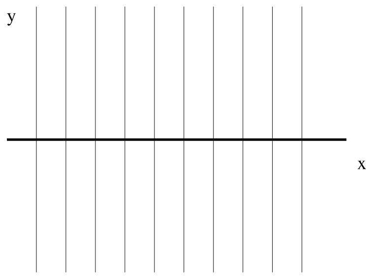 Figure 1
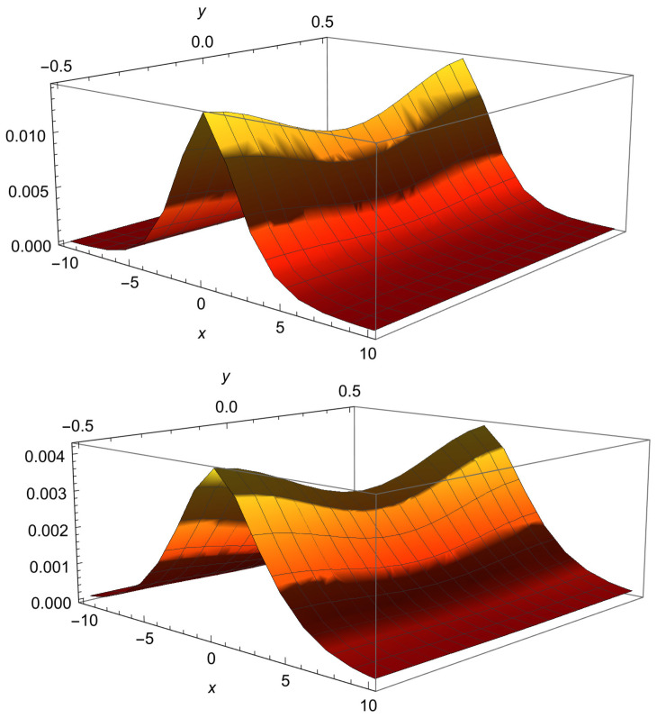 Figure 2
- —Max Planck Institute for the Physics of Complex Systems, Dresden
- —German Science Foundation
- —Alliance of International Science Organizations
- —Alexander von Humboldt Foundation
Peer Reviews
No public reviews on file for this paper yet. If you reviewed it on a platform where reviews are public (OpenReview, ICLR, NeurIPS, ICML), you can paste yours below so the community can read it here.
Videos
No videos yet. Explain this paper in a talk, walkthrough, or lecture? Add one.
Taxonomy
TopicsCoagulation and Flocculation Studies · Particle Dynamics in Fluid Flows · Ionosphere and magnetosphere dynamics
1. Introduction
A comb model, being a specific realization of random loopless structures, is a model of geometrically constrained diffusion. A typical comb, shown in Figure 1, consists of a central backbone along the x axis and infinite side branches (teeth or fingers of the comb) in the y direction. Because combs are loopless objects (similarly to Bethe lattices), they have long been considered as an appealing simplification of percolation clusters [1,2,3]. A remarkable feature about combs is that they capture much of the actually observed signatures of anomalous transport in disordered systems, with side branches being the sources for memory and dynamical traps. In this context, the comb model could be regarded as a geometric representation of the continuous-time random walk [3]. The various aspects of anomalous diffusion on combs have been discussed in [4,5,6,7,8,9,10,11,12,13]. The possible physics applications are reviewed in [14,15,16,17]. A common feature of all these applications is the understanding that the classic random-walk process in comb geometry leads to asymptotic subdiffusion along the backbone, with the mean-squared displacement (MSD) growing with time as . This subdiffusive scaling law has been found in a variety of experimental situations and mathematical models, with theoretical underpinnings pertaining to the percolation problem, the first passage time density problem, trapping-induced diffusion-controlled reactions, interactions through soft pairwise potentials considered within the linearized Dean–Kawasaki framework, and Lévy flights in optics [18,19,20,21,22,23,24]. Among other applications, the finite velocity transport [20,25,26], quenched and annealed disorder mechanisms [27] and non-Markovian quantum phenomena [28] should be admitted as well. Part of the challenge is concerned with biomedical aspects, such as fractional oncology [29,30] and fractional neurology [31,32,33]. Other issues include stochastic resetting with non-equilibrium stationary states realization [34], the various generalizations of the Ornstein–Uhlenbeck process [35,36], and random walks on uniform and non-uniform combs and brushes [12,13,37,38]. Another area of attraction is the one related to layering phenomena in drift–wave plasma (alternatively, beta–plane atmospheric) turbulence [39,40,41,42,43,44,45,46]; see also Ref. [47] for review. The main idea here is that poloidal and radial diffusion in toroidal magnetic confinement systems such as tokamaks and stellarators may couple together to produce long-lived regular patterns of highly concentrated jet zonal flows, the so-called plasma staircase [39,40,41,42,43,44,45], with the coupling agent being identified as turbulence spreading [46].
Here, we consider a simplified version of this complex process and generalize the comb model due to Arkhincheev and Baskin [48] by augmenting it with a periodic potential in fingers. We aim to understand how the potential function added affects the asymptotic transport scalings in the backbone. Subsequently, we show that the relaxation process in fingers leads to a possibility of a non-equilibrium stationary state (NESS) in a comb geometry. The latter distribution is found to be the direct result of relaxation towards stationarity of the Mathieu eigenspectrum.
A mathematically elegant way of the comb model has been suggested in Ref. [48] in the form of the two-dimensional Fokker–Planck equation, which is discussed in the next section. Our aim is to consider the comb model in a periodic potential . For our purpose, we first consider some variation of the comb model, a so-called half-plane comb model, when . To that end, in Section 2, we consider some new results in the framework of the half-plain comb model to shed light on the geometrical description of subdiffusion. In Section 3, the periodic potential is introduced along the y axis. In this case, the length of the fingers can be restricted by the period of the potential, . Usually, this additional topological restriction leads to normal diffusion along the backbone [49]. However, in the presence of the periodic potential, subdiffusion does take place along the backbone. This situation leads to a new possibility of controlling the backbone transport in the comb models in external fields.
2. Half-Plane Comb Model
Let be the probability density function (PDF) of a particle/tracer to be in position with coordinates at time t. Then the half-plane comb model reads
Here, corresponds to the backbone, while are side branches (teeth or fingers) continuously distributed along the backbone. All variables and parameters are taken in dimensionless form, so d is an effective diffusion coefficient in the y direction, while the diffusion coefficient in the x direction is the Dirac delta function . In this case, diffusion in the x direction is possible at only. The boundary conditions at infinity are taken to be zero, namely and . There are various scenarios of the initial and boundary conditions at , which will be specified in what follows in the text. The boundary conditions at will be defined in the subsequent scenarios.
2.1. Half-Plane Comb Model I
Let us first consider the initial condition at , defined as , where . The boundary condition on the backbone at is given by , where for ; that is, the boundary condition is imposed at the initial point of the backbone. In this situation, it is better to discuss the density function (DF) of transporting particles. To some extent, this scenario corresponds to a variation of a standard situation; see, e.g., [50]. Performing the Laplace transform with respect to time, , we have Equation (1) as follows
At the boundary , we have
In Laplace space, the transport along the x and y directions is independent. Then we look for the solution to Equation (2) in the form of the following ansatz
where is the Laplace image of the backbone density.
Let us obtain the equation for the marginal density of the x transport. It reads as follows
Performing integration with respect to y in Equations (2) and (4), and taking into account the boundary conditions at infinity and Equations (2) and (3), we obtain the following equations for the marginal DF
Equation (7) also means that . Then Equation (4) yields
Substituting the relation (8) in Equation (6) and taking into account the boundary condition (7) for the backbone DF, we obtain it in Laplace space as follows:
Therefore, the marginal DF in Laplace space is
To estimate the MSD according to the backbone DF, one needs to normalize the latter, since it is the distribution of the non-conserved number of particles, which increases with time due to the boundary condition at . Therefore, the number of particles in Laplace space is the normalization constant, which reads
Consequently, the normalization reads
Therefore, the MSD along the backbone is
Eventually, the two-dimensional DF of the half-plane comb model (3) is
This integration leads to the convolution of the Gaussian distribution [50] and the Fox H-function [51]; see Appendix B.
An additional correction of the diffusion coefficient for the MSD (12) can also be performed due to the two-dimensional geometry. The number of transporting particles according to the DF (13) is
Then the MSD, according to the 2D PDF, is
2.2. Half-Plane Comb Model II
Let us now consider the half-plane comb model with the non-zero initial condition , and zero boundary condition at , namely . In this case, the strategy of the solution is to determine the Green function for the standard two-dimensional comb model, with an odd initial condition imposed on the entire x axis; that is, and, correspondingly, . Then, the solution for the PDF of the half-plane comb model is the convolution
Therefore, the backbone transport can be described by the marginal PDF and, correspondingly, by the Green function (the marginal transition probability) with the initial condition , according to Equations (16) and (17). It is worth noting that, in this boundary value problem, the number of particles is conserved. Then, the backbone solution (16) for the half-plane comb model can be presented by the chain of simple transformations,
where . Then the Fourier transform with respect to x yields
2.3. Green Function
Let us first solve the equation for the comb Green function with the initial condition . Then, the standard comb equation for the Green function reads
The zero boundary conditions are at infinity.
Performing the Laplace transform and looking for the solution in the form of an ansatz (4), we have
where . Integrating Equations (20) and (21) with respect to y, where , we have in Laplace space
and
Then, replacing in Equation (22) by means of Equation (23) and performing the Fourier transform, we obtain the x-Green function in Fourier–Laplace space as follows:
where we set . Then, the Fourier image of the Green function is expressed in the form of the Mittag–Leffler function [52],
2.4. Half-Plane Comb Model II: MSD
Taking into account Equation (19), we obtain the Fourier–Laplace image of the marginal PDF of the half-plane comb model as follows:
The inverse Fourier–Laplace transform yields
Here, the Fox H-function (A4) is obtained by means of the Mellin–Barnes integral; see Appendices Appendix A and Appendix B.
As admitted above, in the second scenario of the half-plane comb model, the number of particles is conserved. The latter is determined by the initial condition . From Equation (26) we have
which is the normalization constant for the PDF, where is the Heaviside theta function.
3. Side-Branched Periodic Potential
As shown above, the consideration of the half-plane comb model eventually reduces to the standard analysis of the two-dimensional comb model, where the boundary conditions on the backbone at are unnecessary and can be discarded. In this case, corresponds to the backbone. Let be the PDF of a particle/tracer being at the position with coordinates at time t. Then, the comb model in a periodic potential reads
where and are diffusion coefficients in the x and y directions, respectively. The periodic potential is defined as , the prime means derivative with respect to y, and is the amplitude of the periodic variation. Here, a is the period of the potential, which describes the effective length of the side branches.
All variables and parameters can be taken in the same dimensionless form as in Equation (1) by introducing the scaling parameters for time, with and for the spatial coordinates, with , and , and . Note that has the dimension of the diffusion coefficient as well. The amplitude of the periodic potential can also be considered in dimensionless form by scaling . The latter scaling reflects the fact that the dimensionless . After rescaling, the periodic potential reads . Eventually, the dimensionless form of Equation (28) reads
The boundary conditions at infinity are taken to be zero, namely and . Note also that the side-branched boundary conditions in the presence of the periodic potential will be redefined as necessary; namely, these boundaries can be considered at half of the period of the periodic potential. The initial condition now is .
and substituting it in Equation (29), we obtain the following equation:
where . In particular, if , then
Following the standard procedure [16,48], we perform the Laplace transform of Equation (31) with respect to time and look for the Laplace image in the form of the ansatz
Note that this ansatz differs from the standard one defined in Equations (4) and (21) by an additional side-branched function . Substituting Equation (33) in the Laplace transform of Equation (31), we obtain the following equation:
where is the sign function of y. This equation can be divided into two equations by separating terms with the Dirac delta function that corresponds to the backbone transport at from the terms valid for that correspond to the side-branched transport . Thus, we have
which is the backbone equation, where . The second equation follows immediately from Equation (34) for . It determines an additional function, which appears in the analysis due to the periodic potential and for it reads
First, we consider the backbone transport.
3.1. Backbone Transport
Performing the Fourier transform of the backbone Equation (35), we have
that yields
Performing the Fourier inversion, we obtain
Substituting solution (39) in Equation (35), one verifies the correctness of the analysis.
3.2. Side-Branched Transport: Mathieu Equation
The side-branched Equation (36) is symmetrical with respect to inversion . Therefore, for , it reads in the form of the ordinary differential equation as follows:
To simplify the consideration without restriction of generality, we take into account that in the periodic potential , the parameter is small. Then, neglecting the term with in Equation (32), we obtain the following:
where . Note that this simplification of does not change its period. To arrive at the Mathieu equation, we make the substitution and then define . That yields
Note also, considering this equation symmetrically, the second derivative of the term does not contain the delta-function, since for .
Following the standard definition [55,56], we arrive at the Mathieu equation:
where and . Floquet theorem [55,56], ensures the solution
with the property , where is the quasi-energy (also known as the characteristic exponent). It relates to the eigenvalues of the Mathieu Equation (43) as follows [55,56]: . This situation is unique when the Mathieu spectrum is proportional to the inverse time and tends to zero with time as . Considering the large-time dynamics when , we find that, for , the only reasonable solution is the Mathieu function , which is positive for and has the spectrum [55,56,57]. However, without restriction of the transport properties, we restrict the dynamics by boundaries that make the integration with respect to y feasible in Equation (46). For small values of the parameter q, which is exactly our case, this Mathieu function has a simple form of the positive periodic function [55]
Eventually, we arrive at the stationary state, which is the non-equilibrium stationary state (NESS) [58] of the relaxation process in the side-branched part of the comb system. Taking into account that is a symmetrical function, we obtain it as follows:
This also yields .
3.3. PDF of the Comb Model
Collecting the results of this section for the comb PDF given in Equations (28) and (29), we first present its Laplace-image form as follows:
where is the Laplace image of the standard comb model, considered in Section 2. This result can be easily extended to the half-plane comb model, considered in Section 2.1, by taking into account that the half-plane comb PDF is according to Equation (13). Note also that in this case, the number of transporting particles is not conserved due to the constant source term at the boundary with .
The contribution of the side-branched periodic potential to the backbone transport reduces to the additional multiplication by the NESS, which is the side-branched exponential and the Mathieu function, .
The asymptotic comb PDF is
which consists of subdiffusion along the backbone and asymptotic ( ) NESS along the fingers. In this case, to normalize the PDF, the boundary conditions for the fingers should be reformulated and taken to be free boundary conditions at . Eventually, it results in the direct product of the periodic in the y stationary distribution and the Fox H-function, as considered in Appendices Appendix A and Appendix B. Consequently, the Fox H-function here results from the inverse Laplace transform and is given by
see Equation (A3), where we use and . Graphical representation of the relaxation process at the large time asymptotics is shown in Figure 2, which pertains to Equations (48) and (49). Therefore, the scaling variable is , and the MSD along the backbone is
This result leads to subdiffusion, since the total probability on the backbone is not conserved.
Therefore, the MSD reads .
4. Summary
In this paper, a comb model with a periodic potential in fingers has been considered. Our main findings can be summarized as follows. Firstly, we have shown that the periodic motion in fingers affects the anomalous diffusion along the backbone, leading, under appropriate boundary conditions, to the occurrence of a non-equilibrium stationary state (NESS). Secondly, we have seen that the distribution of the probability density in the vicinity of NESS is given by a variant of the Mathieu function. Thirdly, we have inferred the asymptotic transport scalings for the backbone transport (Section 2.1) and showed that the transport is subdiffusive, with the mean-squared particle displacement growing with time as . These basic findings need to be augmented with some explanatory notes as follows.
Our first note here is concerned with the side-branched process described by Equation (41), with the solution . By its construction, Equation (41) describes the particle motion within the interval . The point is excluded from the consideration, since the corresponding term belongs to the backbone dynamics and is taken into account in Equation (35) for . However, in the final PDF (48), the Mathieu function is already defined at , as well, since the final expression (48) is valid for all values of y, which is also taken into account by .
The infinite strip , where the periodic potential affects the comb diffusion, is leaked at the boundaries . This results from the periodicity of the stationary distribution , when . Therefore, there are free boundary conditions for the fingers. It should be pointed out that this stationary solution is asymptotic and valid for large times, since initially it is a superposition of a complete set of the Mathieu functions, which form the initial function due to the completeness property of the periodic Mathieu functions [59]. However, as follows from Equation (41), the spectrum is negative; that is, it is bound, and tends to zero for the large-time ( ) asymptotics. As a result, this periodic asymptotic solution is described by the Mathieu function .
Last but not least, it is suggested that the proposed comb model mimics the defining features of anisotropic transport in beta–plane atmospheric (drift–wave plasma) turbulence. Support for this suggestion can be found in the analysis of Refs. [45,46], where one associates the y direction with the direction along the flow, and the x direction with the direction perpendicular to the flow. In this context, the comb model provides a simplified yet relevant theoretical framework to characterize the inherent coupling between turbulent degrees of freedom, with the periodic potential along the y direction affecting the anomalous transport along the x direction. The finding above that the MSD along x grows with time as can be supported by the results of computer simulations of drift–wave anisotropic plasma turbulence, reported in [60,61].
Developing these viewpoints, one might further associate the NESS solutions of the comb model with turbulence-dominated, long-lived layered structures, zonal flows and staircases, see Ref. [47] and references therein. In this context, the periodic potential in fingers has a very clear physical interpretation: it captures the extra harmonics (in the poloidal cross-section) resulting from bending into a torus of otherwise cylindrically symmetric magnetic flux surfaces, the so-called shape effect (and thus the effect of toroidicity and flux-surface shaping on the poloidal plasma convection in a tokamak, e.g., Ref. [62]). Also, in the optics of NESS, it emphasizes the crucial role of toroidal geometry in the occurrence of layered structures and staircases; see Refs. [41,42,45].
Overall, the comb model opens up a new perspective on the study of staircase self-organization using fundamental methods. Extending this study to fluid (and fluid-like, such as electrostatic drift–wave) applications might be strongly advocated. In this connection, we would like to remark that the comb model correctly describes the transport of drift waves in a reactor-relevant setup of fusion plasma [46].
The reference list from the paper itself. Each links out to its DOI / PubMed record.
- 1White S.R. Barma M. Field-induced drift and trapping in percolation networks J. Phys. A Math. Gen.1984172995300810.1088/0305-4470/17/15/017 · doi ↗
- 2Gefen Y. Goldhirsch I. Biased diffusion on random networks: Mean first passage time and DC conductivity J. Phys. A Math. Gen.198518 L 1037 L 104110.1088/0305-4470/18/16/008 · doi ↗
- 3Weiss G.H. Havlin S. Some properties of a random walk on a comb structure Phys. A 198613447448210.1016/0378-4371(86)90060-9 · doi ↗
- 4Baldi G. Burioni R. Cassi D. Localized states on comb lattices Phys. Rev. E 20047003111110.1103/Phys Rev E.70.03111115524510 · doi ↗ · pubmed ↗
- 5Baskin E. Iomin A. Superdiffusion on a Comb Structure Phys. Rev. Lett.20049312060310.1103/Phys Rev Lett.93.12060315447248 · doi ↗ · pubmed ↗
- 6Dvoretskaya O.A. Kondratenko P.S. Anomalous transport regimes and asymptotic concentration distributions in the presence of advection and diffusion on a comb structure Phys. Rev. E 20097904112810.1103/Phys Rev E.79.04112819518194 · doi ↗ · pubmed ↗
- 7Iomin A. Subdiffusion on a fractal comb Phys. Rev. E 20118305210610.1103/Phys Rev E.83.05210621728596 · doi ↗ · pubmed ↗
- 8Forte G. Burioni R. Cecconi F. Vulpiani A. Anomalous diffusion and response in branched systems: A simple analysis J. Phys. Condens. Matter 20132546510610.1088/0953-8984/25/46/46510624153224 · doi ↗ · pubmed ↗