Lyapunov Thermodynamic Stability of the Evolution of Conservatively Perturbed Chemical Equilibrium
Anil A. Bhalekar, Vijay M. Tangde, Bjarne Andresen

TL;DR
This paper shows that a simple chemical equilibrium system remains stable over time when slightly disturbed.
Contribution
The study proves asymptotic thermodynamic stability in a two-step reversible reaction using Lyapunov methods.
Findings
Systems with conservatively perturbed chemical equilibrium are asymptotically thermodynamically stable.
Lyapunov thermodynamic stability formulation confirms long-term stability in such reactions.
Abstract
The thermodynamic stability of the evolution of a simple conservatively perturbed chemical equilibrium, that is, a two-step reversible reaction, is investigated using the Lyapunov thermodynamic stability formulation. We show that such systems are asymptotically thermodynamically stable.
Genes, proteins, chemicals, diseases, species, mutations and cell lines named across the full text — each resolved to its canonical identifier and authoritative record.
Click any figure to enlarge with its caption.
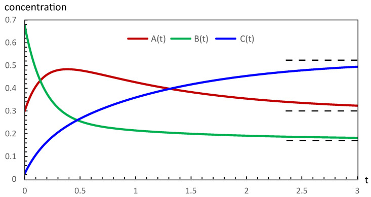 Figure 1
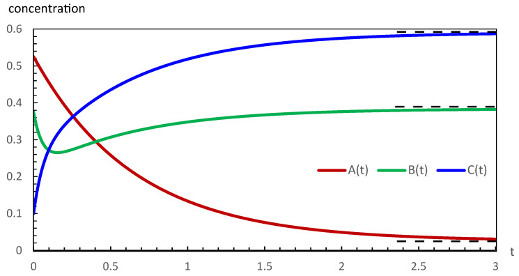 Figure 2
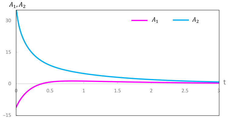 Figure 3
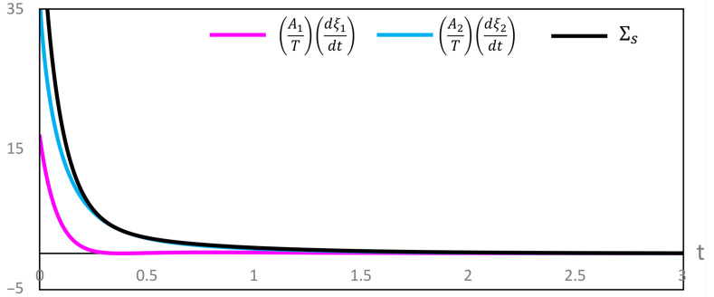 Figure 4
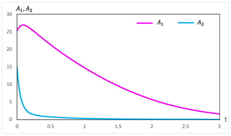 Figure 5
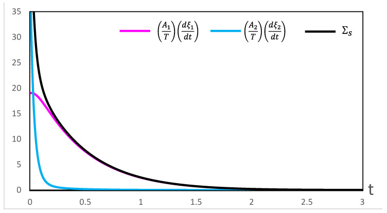 Figure 6
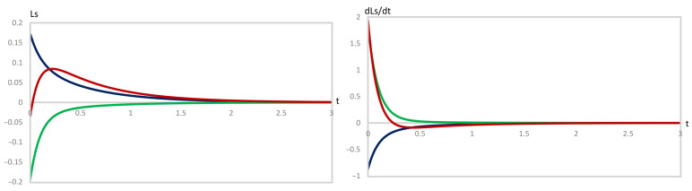 Figure 7
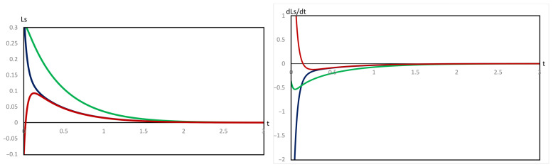 Figure 8
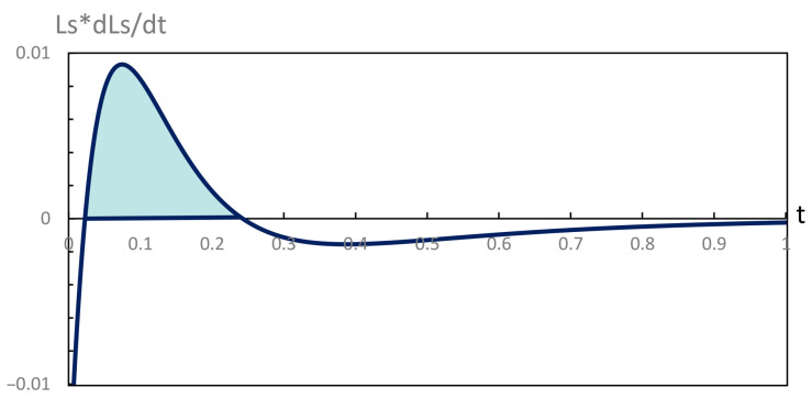 Figure 9
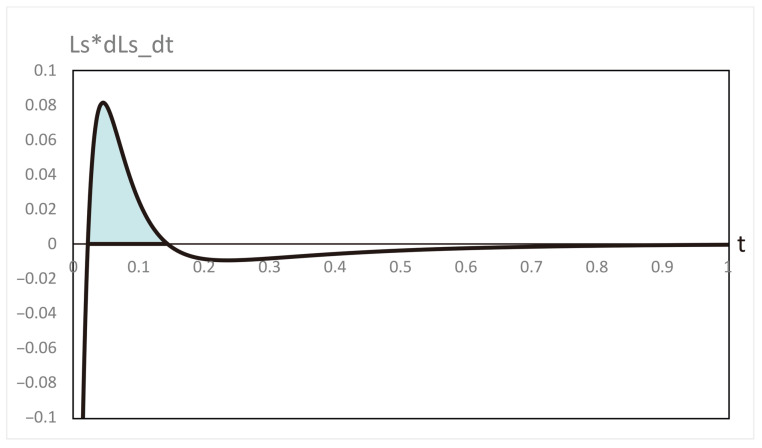 Figure 10
Peer Reviews
No public reviews on file for this paper yet. If you reviewed it on a platform where reviews are public (OpenReview, ICLR, NeurIPS, ICML), you can paste yours below so the community can read it here.
Videos
No videos yet. Explain this paper in a talk, walkthrough, or lecture? Add one.
Taxonomy
TopicsAdvanced Thermodynamics and Statistical Mechanics · stochastic dynamics and bifurcation · Nonlinear Dynamics and Pattern Formation
1. Introduction
In our recent publication [1], we described our thermodynamic theory, named Lyapunov thermodynamic stability (LTS), for analyzing the stability of irreversible processes on a generalized footing. This theory uses all the ingredients of Lyapunov’s second method of stability of motion [2,3,4]. The needed Lyapunov function is defined via the rate of entropy production, which is an inseparable property of irreversibility. This theory has been used to establish thermodynamic stability aspects of various irreversible processes, including some of industrial importance [5,6,7,8,9,10,11,12,13].
Recently, a new chemical kinetics tool has been developed, named conservatively perturbed equilibrium (CPE) [14,15,16]. In it, a system is allowed to attain chemical equilibrium. The concentrations of some of the reacting species are then conservatively perturbed while keeping the temperature, pressure, and concentration of at least one chemically reacting species unaltered, and its progress toward the same equilibrium is followed. It is observed that the concentrations of unperturbed species pass through extrema (minima or maxima) before finally attaining their original equilibrium concentrations. It is precisely this extremal out-of-equilibrium feature at some point along the equilibration that makes CPE interesting in practical situations.
A priori, it is possible that the production of such extrema in a CPE evolution makes the corresponding trajectory thermodynamically unstable. To investigate this possibility, we performed an LTS stability analysis of the simplest CPE system. Our results show that such perturbed trajectories are not merely thermodynamically stable but are asymptotically thermodynamically stable.
2. Evolution of Conservatively Perturbed Equilibrium and the Rate of Entropy Production
For simplicity in our presentation, we consider the following two-step reversible consecutive reaction scheme:
where , , and are the chemically reactive species and are the respective rate constants. Thus, the rates of reaction in terms of the respective extent of the advancement of reaction, , are
i.e., the number of moles of A converted to B for the first reaction, and the number of moles of B converted to C for the second reaction since the start of the experiment ( ) (see, for example, [17,18]).
Therefore, we have,
The respective concentrations are also denoted by A, B, and C in the above rate expressions. In the case of the chemical reaction in Equation (1), the CPE has been studied in two ways [15]. In the first case, A starts at its equilibrium concentration , and the concentrations of B and C are perturbed under the condition . In the second case, B starts at its equilibrium concentration with perturbations . The plots of the respective evolutions to the final equilibrium states in the above two cases are shown in Figure 1 and Figure 2.
Throughout this paper, standard SI units are used for the numerical calculations. Thus, time is shown in sec, concentrations in M (molar), affinities in J/mol, and entropy production rates in W/K.
The variation of the concentration A in Figure 1 tells us that initially, the first step proceeds from right to left (implying ), and beyond the maximum, the step reverses direction (implying ). The second step throughout proceeds from left to right (implying ).
In the case of the evolution in Figure 2, at the initial stages, the decrease in the concentration of A is less steep than the increase in the concentration of C. This means that the rate of production of B in the first step of the reaction is exceeded by a much more rapid consumption of B in the second step. Therefore, both steps of the reaction in Equation (1) throughout proceed from left to right, implying and .
A consecutive two-step reversible reaction has the following rate of entropy production [19,20,21]:
where T is the temperature of the system and are the respective chemical affinities, which have the following standard expressions in the present case:
where are the respective chemical potentials. The overall positive sign of (5) is guaranteed by the second law of thermodynamics [18]. The thermodynamic expressions of chemical affinities, assuming ideality of the reaction mixture, are
where the superscript ⦵ denotes the chosen standard state and R is the universal gas constant. Since at equilibrium, chemical affinities are equal to zero, this provides the following expressions for standard-state chemical affinities:
Therefore, Equation (5), on using the expressions of Equations (2), (3), (7), and (8), becomes
Notice that each term of Equation (9) is individually positive, since when , we have , and when , we have . The same argument applies to the second term of Equation (9). Therefore, is never negative at any point in the evolution of the CPE.
Our computations of thermodynamic properties corresponding to the evolutions depicted in Figure 1 and Figure 2 are presented in Figure 3, Figure 4, Figure 5 and Figure 6. All calculations are carried out at K. It can be seen in Figure 3 that the variation of the chemical affinities of the two steps is commensurate with the respective behavior of the two steps depicted in Figure 1. That is, the chemical affinity of the second step, , remains positive throughout and continuously decreases (this step maintains the direction left to right throughout). In contrast, the chemical affinity of the first step, , is initially negative (the initial direction of this step is right to left), becomes zero at the maximum of A, and then becomes positive (the direction of the step becomes left to right). Both chemical affinities finally become zero on attaining chemical equilibrium. In spite of this change of direction, Figure 4 illustrates that both rates of entropy production, and , remain positive throughout, decreasing eventually to zero. Therefore, the sum of these two terms, that is , also remains positive throughout and continuously decreases, as expected. A similar explanation follows for Figure 5 and Figure 6.
Thus, we see that each step of the reaction in Equation (1) during the evolution depicted in Figure 1 and Figure 2 follows the thermodynamically favorable direction with positive entropy production, as set out in Equation (5). This means that the steps remain thermodynamically uncoupled under the conservatively perturbed evolution, i.e., at no point does one reaction drive the other.
3. Lyapunov Thermodynamic Stability of the Evolution of Conservatively Perturbed Equilibrium
Lyapunov thermodynamic stability (LTS) theory uses a sign-definite thermodynamic Lyapunov function, (refer to, for example, [1]), to analyze the nature of the thermodynamic stability of an irreversible process. The steps of the adopted approach are as follows:
- 1.Effect a sufficiently small perturbation at a desired time ( ) on the trajectory of an evolution whose stability is under investigation.
- 2.As a result of this perturbation, the system follows a perturbed trajectory.
- 3.Follow the course of the perturbed trajectory under the same conditions as for the unperturbed one. If within a reasonably short time it reverts to the unperturbed trajectory, the latter is called asymptotically thermodynamically stable; if eventually it ends up only in the close vicinity of the unperturbed one, then the latter is termed thermodynamically stable; and if the perturbed trajectory diverges away from the unperturbed one, then the latter is established as a thermodynamically unstable motion.
- 4.Along the lines of the Lyapunov second method, these conclusions in LTS are arrived at via the signs of and its time derivative, . The basic requirement of is that it should depend on the perturbation coordinates and time, as well as vanish only on the unperturbed trajectory (the latter is also called the origin). If is of the opposite sign (i) and vanishes only at the origin, then the latter is obtained as asymptotically thermodynamically stable, or else (ii) if it vanishes without reaching the origin, then the latter is established as a thermodynamically stable motion. In the case of thermodynamically unstable motion, we have the same signs of the Lyapunov function and its time derivative.
3.1. Thermodynamic Lyapunov Function of LTS and Stability Criteria
The mathematical expression for in LTS is chosen as
where is the rate of entropy production on the perturbed trajectory and is that on the unperturbed trajectory. We denote the quantities pertaining to the unperturbed trajectory by the superscript 0. Recall that the second law of thermodynamics guarantees the positive definite sign of the rate of entropy production. One can refer to as the perturbation gain of entropy production or excess entropy production due to perturbation. It is possible that upon perturbation, the rate of entropy production decreases instead of the increase shown in Equation (10). If this occurs, all the arguments about stability here and below, assuming , can be directly converted to , with all subsequent inequalities reversed, as long as its time derivative, , also changes its sign, i.e. becomes positive, since the requirement for Lyapunov stability is that the product is negative.
The rate of entropy production depends on the thermodynamic variables appearing in the corresponding Gibbs relation, such as T, p, and the composition variables. Alternatively, one can use the generalized fluxes as the thermodynamic variables. Let the thermodynamic variables be denoted by on the perturbed trajectory and by on the unperturbed trajectory. The perturbation coordinates are defined as
with the condition , where indicates a sufficiently small neighborhood about the origin. Therefore, the unperturbed trajectory is expressed as
with the condition , where indicates another sufficiently small neighborhood about the origin for the initial perturbation.
Let the differential equations on the unperturbed trajectory be
and those on the perturbed trajectory be
The differential equations governing the perturbation coordinates, from Equations (11)–(14), are
Thus, for a non-autonomous system, we have the following functional dependence:
Notice that vanishes on the unperturbed trajectory, which, from Equations (10) and (12), gives
Next, the time derivative of is
Therefore, along the lines of the Lyapunov second method for the stability of motion [2,3,4], we have the following thermodynamic stability criteria:
- 1.Thermodynamic stability is expressed as
That is, may vanish before the perturbed trajectory reaches the unperturbed one.
- 2.Asymptotic thermodynamic stability is described as
That is, vanishes only on the unperturbed trajectory.
3.2. The Basic Expressions for Analyzing the Thermodynamic Stability of the Evolution of Conservatively Perturbed Equilibrium
In the stability analysis, the perturbations have to be sufficiently small; hence, we represent the perturbations in the concentrations as , , and under the condition of conservation of mass given by
The concentrations on the perturbed trajectory are expressed as
Next, using the expressions in Equations (21) and (22) in the rate expressions of Equations (2)–(4), the differential equations for the perturbation coordinates become
Notice that in light of the mass balance condition in Equation (21), we have only two independent perturbation coordinates; hence, only two corresponding differential equations are needed.
Now we introduce the perturbations in Equation (22), the mass balance in Equation (21), and the assumption that , , and into the rate of entropy production on the perturbed trajectory, Equation (9), to obtain
Similarly, Equation (9) for the unperturbed trajectory becomes
Therefore, the expression for , as defined in Equation (10), is obtained from Equations (25) and (26), after a little algebra, as
with
and
Notice that the coefficients and in Equation (27) have their respective expressions in terms of time-dependent quantities belonging to the unperturbed trajectory. Hence, at constant and , still varies with time. This constitutes a non-autonomous system because we have .
The time rate of from Equation (27), and on using Equations (23) and (24), becomes
4. Results and Discussion
4.1. Plots of LS and LS˙ Under Various Choices of Perturbation
We studied the thermodynamic stability aspects of the trajectories depicted in Figure 1 and Figure 2 against sufficiently small perturbations under the mass conservation condition in Equation (21). These small perturbations, applied for the purpose of stability analysis, should not be confused with the larger perturbations of M applied at time as part of the conservatively perturbed equilibrium (CPE) schedule. The sufficiently small perturbations are superimposed on the CPE. The small perturbations were effected at five different stages (times) of each evolution in Figure 1 and Figure 2. The stages chosen are (a) beginning, (b) left side of the extremum, (c) at the extremum, and (d) and (e) on the right side of the extremum, where the CPE trajectories achieved the concentrations listed as , and . Due to mass conservation, these small perturbations always add up to zero, .
The full set of the 30 systems investigated is summarized in Table 1 and Table 2. Out of these, three representative situations, each at the A maximum (Figure 1) and at the B minimum (Figure 2), are presented in Figure 7 and Figure 8. At these points, we focus on cases of perturbation in a Lyapunov sense at times when an extremum is observed in the CPE evolution, i.e., at stages named c in the tables. The full set of plots is available on request from Dr. Vijay Tangde [email protected].
4.2. Discussion
The sets of perturbations effected using the mass conservation condition in Equation (21) and studied for the thermodynamic stability of the evolutions presented in Figure 1 and Figure 2 are summarized in Table 1 and Table 2, respectively.
In the case of the evolution in Figure 1, we have the effected perturbations (i) , , , (ii) , , , and (iii) , , . These perturbations were effected before the maximum of A, at the maximum of A, and beyond the maximum of A. Thus, a total of 15 pairs of plots of and were generated.
In case (i), for all instances studied, the values of these two functions satisfy and , and both vary continuously and finally vanish at the origin. In case (ii), the signs are reversed, and , while both still vary continuously and finally vanish at the origin. Thus, in these cases, asymptotic thermodynamic stability is established. Case (iii) is different. It does eventually display asymptotic thermodynamic stability, like cases (i) and (ii), because and have opposite signs and finally both vanish at the origin. But, during short initial time periods, and have the same sign, creating a temporary state of instability (representative plots of all three cases are depicted in Figure 7).
Notice that along the black and green curves in Figure 7, and are of opposite signs, and thus consistently, as required for stability, and they smoothly vanish at large t on the unperturbed trajectory. This establishes the asymptotic thermodynamic stability of the unperturbed trajectory against these perturbations. Applying perturbations , , and yields a different behavior. The resulting variations of and are depicted as the red curves in Figure 7. During a short initial time period, and both change signs, but at slightly different times, and consequently exhibit a brief period of instability.
Subsequently, opposite signs are restored, and the Lyapunov curve continues toward a zero value on the unperturbed trajectory. Thus, during this short initial interval, , implying instability, as depicted in light blue in Figure 9. This means that the perturbed trajectory passes through a transient instability during the short initial time period but finally approaches the unperturbed trajectory asymptotically, thereby demonstrating asymptotic thermodynamic stability.
In the case of the evolution in Figure 2, the effected perturbations are (i) , , , (ii) , , , and (iii) , , . These perturbations were effected before the minimum of B, at the minimum of B, and beyond the minimum of B.
In this case, we also generated 15 pairs of plots. For all cases of (i) and (ii), we have and throughout, and both finally vanish at the origin. Hence, against these perturbations, the evolution in Figure 2 is established as asymptotically thermodynamically stable. The black and green curves in Figure 8 are representative plots of cases (i) and (ii) when the perturbation is effected at the minimum of B.
Likewise, in case (iii), barring a very short initial time period, we observe that and throughout, and they vanish only at the origin. Hence, the evolution in Figure 2 against the perturbation of type (iii) is established as asymptotically thermodynamically stable. However, in this case, at the initial stages, for a short time period where , the system passes through a transient instability. The red curve in Figure 8 shows such a perturbation effected at the minimum concentration of B. The brief period of instability is depicted in Figure 10, analogous to Figure 9.
It is worth emphasizing that the two systems producing transient instability have a common feature. Recall that the CPE evolution in Figure 1 is obtained when the concentration of A is unperturbed, whereas the evolution in Figure 2 is generated when the concentration of B is unperturbed. In both cases, the signs of the perturbations in the concentrations of the respective other two species ( and in the former case, and and in the latter case), in the Lyapunov sense, are opposite to the signs of the perturbations effected on A (in the former case) and B (in the latter case).
5. Conclusions
The overall conclusion is that the evolutions of conservatively perturbed chemical equilibrium in a two-step consecutive chemical reaction are asymptotically thermodynamically stable despite producing extrema in the concentration of the unperturbed reactive species.
In general, from a chemical kinetics point of view, a conservatively perturbed setup is equivalent to studying kinetics with, for example, initial concentrations , and or , and , with the respective conditions and . The two cases of CPE investigated in the present work are depicted in Figure 1 and Figure 2. Of course, we can see that in the former case, the first step initially proceeds from right to left, and after the attainment of the maximum concentration of A, it changes its direction, while the second step maintains its direction from left to right throughout. In contrast, in the latter case, despite the observation of a minimum in the concentration of B, both steps maintain their direction from left to right throughout. Despite the observation of extrema in the concentration of unperturbed species and the change of direction of the first step in Figure 1, these CPE evolutions are proven to be asymptotically thermodynamically stable. This conclusion strengthens the thermodynamic notion that such unusual-looking behavior does not influence stability, provided the second law of thermodynamics is not violated.
In future studies, using the same line of reasoning, we will investigate the thermodynamic stability of more complex CPE systems whose chemical kinetics have already been carried out [14,15].
The reference list from the paper itself. Each links out to its DOI / PubMed record.
- 1Tangde V.M. Bhalekar A.A. Andresen B. Thermodynamic Stability Theories of Irreversible Processes and the Fourth Law of Thermodynamics Entropy 20242644210.3390/e 2606044238920451 PMC 11202706 · doi ↗ · pubmed ↗
- 2Chetayev N.G. The Stability of Motion 1st ed.Pergamon Press Oxford, UK 1961
- 3Elsgolts L. Differential Equations and the Calculus of Variations Yankuvsky G. Mir Publications Moscow, Russia 1970
- 4La Salle J.P. Lefschetz S. Nonlinear Differential Equations and Nonlinear Mechanics Academic Press New York, NY, USA 1963
- 5Bhalekar A.A. On a Comprehensive Thermodynamic Theory of Stability of Irreversible Processes: A Brief Introduction Far East J. Appl. Math.20015199210
- 6Bhalekar A.A. Comprehensive Thermodynamic Theory of Stability of Irreversible Processes (CTTSIP). I. The Details of a New Theory Based on Lyapunov’s Direct Method of Stability of Motion and the Second Law of Thermodynamics Far East J. Appl. Math.20015381396
- 7Bhalekar A.A. Comprehensive Thermodynamic Theory of Stability of Irreversible Processes (CTTSIP). II. A Study of Thermodynamic Stability of Equilibrium and Nonequilibrium Stationary States Far East J. Appl. Math.20015397416
- 8Bhalekar A.A. Burande C.S. A Study of Thermodynamic Stability of Deformation in Visco-elastic Fluids by Lyapunov Function Analysis J. Non-Equilib. Thermodyn.200530536510.1515/JNETDY.2005.004 · doi ↗