Surface Tension Isotherms: Reconceptualizing Adsorption, Self-Assembly, and Micelle Formation via the Fluctuation Theory
Seishi Shimizu, Nobuyuki Matubayasi

TL;DR
This paper introduces a new theory that explains how surfactants behave at interfaces and in solutions using surface tension isotherms and fluctuation theory.
Contribution
A novel fluctuation-based theory is proposed to redefine surfactant aggregation and adsorption without relying on traditional stoichiometric models.
Findings
The gradient and curvature of surface tension isotherms reveal interactions between surfactant sorption and bulk fluctuations.
The new ABC isotherm generalizes the Szyszkowski–Langmuir model by capturing surface–bulk differences in surfactant correlations.
The theory replaces the 'area-per-molecule' concept with a projected area that includes interface thickness.
Abstract
Given a surface tension isotherm (i.e., how interfacial free energy changes with the surfactant concentration), can we gain insight into how surfactant molecules interact at the interface and in the bulk solution? Historically, surfactants were modeled to bind onto a uniform interface, before aggregating stoichiometrically at the critical micelle concentration (CMC). However, this simple model contrasts with counterevidence, e.g., premicelles (smaller aggregates below CMC) and aggregate size distribution, necessitating a departure from stoichiometric aggregation models. To this end, a novel theory for surface tension will be established by synthesizing the statistical thermodynamic fluctuation theory for sorption and self-assembly in solution. This theory provides a link between the functional shape of a surface tension isotherm and the underlying interactions. We demonstrate that the…
Genes, proteins, chemicals, diseases, species, mutations and cell lines named across the full text — each resolved to its canonical identifier and authoritative record.
Click any figure to enlarge with its caption.
 1
1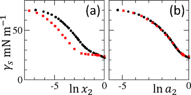 2
2 3
3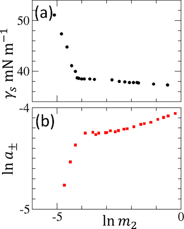 4
4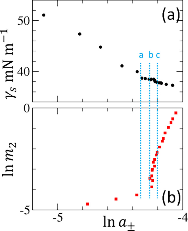 5
5 6
6 7
7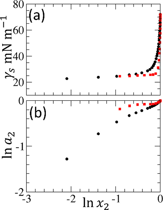 8
8 9
9 10
10| parameter range | isotherm equation |
|---|---|
|
|
|
|
| |
|
|
|
|
|
|
|
|
|
- —Maruho10.13039/100030684
- —Ministry of Education, Culture, Sports, Science and Technology10.13039/501100001700
- —Ministry of Education, Culture, Sports, Science and Technology10.13039/501100001700
- —Ministry of Education, Culture, Sports, Science and Technology10.13039/501100001700
- —Steven Abbott TCNF LtdNA
Peer Reviews
No public reviews on file for this paper yet. If you reviewed it on a platform where reviews are public (OpenReview, ICLR, NeurIPS, ICML), you can paste yours below so the community can read it here.
Videos
No videos yet. Explain this paper in a talk, walkthrough, or lecture? Add one.
Taxonomy
TopicsSurfactants and Colloidal Systems · Pickering emulsions and particle stabilization · Polymer Surface Interaction Studies
Introduction
The surface tension of the air/water interface changes with the concentration of the surfactant (“surface tension isotherm”). ?−? ? How can we understand the functional shape of a surface tension isotherm (Figure) on a mechanistic basis, in terms of the underlying surfactant interactions at the interface and in the bulk solution? To answer this question with clarity, this paper proposes to replace the classical models of surface tension (based on stoichiometric aggregation and binding) ?−? ? ? with the statistical thermodynamic fluctuation theory. ?,? This proposal has been necessitated by the mounting evidence for non-stoichiometric behavior in (1) self-aggregation in the bulk (e.g., micelle formation) and (2) adsorption at air/water interface, which poses difficulties for the stoichiometric models for binding and association, as well as by (3) the interpretive difficulties caused by the oversimplifications in capturing 1 and 2, as will be summarized below.
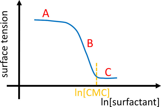
Schematic representation of a surface tension isotherm of surfactant–water mixture against the logarithmic surfactant concentration, with the regions defined by Menger et al. In region A, “the surface tension remain(s) relatively constant”. In region B, or the linear region (concentrations below CMC), “the slope of the curve is essentially constant”. In region C, above the critical micelle concentration, the surface tension levels off.
Capturing Self-Assembly in the Bulk Solution
Surfactants
Surfactant self-assembly cannot be captured by the stoichiometric m-mer formation ?,? that occurs abruptly at the critical micelle concentration (CMC). Evidence abounds that is contrary to the stoichiometric model: (i) premicelles (smaller surfactant aggregates) below CMC ?−? ? and (ii) micellar size distribution, ?,?,?,? namely, the statistical distribution of the aggregation number. Consequently, the surfactant self-assembly must be captured with appreciation of the variability and fluctuation of the aggregation number.
Different Aggregation Theories
for Surfactants and Non-surfactants
Common experimental techniques (e.g., small-angle scattering) have been established to quantify aggregation behaviors across varying degrees of self-association, such as co-solvents and hydrotropes ?−? ? ? as well as surfactants ?−? ? ? in water. However, different theories and models are used for these three classes. For co-solvents and hydrotropes, ?−? ? ? their weak, non-specific, and non-stoichiometric aggregation can be captured ?−? ? ? through the Kirkwood–Buff integral (KBI),? defined via radial distribution functions between molecular species, founded on statistical thermodynamic fluctuation theory. ?−? ? ? For surfactants, in contrast, aggregation numbers, founded on stoichiometric models, are still the common language. ?−? ? ? ? ? ? Despite long-standing attempts to introduce the fluctuation theory for micelles, ?−? ? ? stoichiometric binding models are still commonly used to capture surfactant aggregation, especially in the context of surface tension. ?,?,? Therefore, following previous attempts, ?−? ? ? our goal is to establish the fluctuation theory as the common theoretical foundation across the spectrum of self-association, applicable to co-solvents, hydrotropes, and surfactants alike.
Capturing Adsorption
on Air/Water Interface
What Constitutes a Full Surface Coverage?
To understand a surface tension isotherm mechanistically, not only surfactant aggregation in the bulk, but also surfactant adsorption onto the interface, must be considered. ?−? ? To this end, the Gibbs adsorption isotherm plays a crucial role, which relates the gradient of a surface tension isotherm (plotted against the logarithmic surfactant concentration) to the adsorption capacity of surfactants? (i.e., the number of surfactants adsorbed per area). Therefore, the commonly observed linear region in the surface tension isotherm (Figure) can be attributed to the adsorption capacity reaching saturation. ?−? ? To understand more microscopically the surface coverage of surfactants at saturation, the area-per-molecule is a useful measure to obtain a microscopic picture of surface coverage, easily calculable as the inverse of the saturation capacity (“the number of surfactants per area”).? However, the area-per-surfactant data, collected extensively (see, e.g., Table 2.1 by Rosen and Kunjappu?) in the literature, have recently been questioned by Menger and co-workers. ?,?,? The area values seemed too large [“[i]n order to achieve large surface tension reductions (typically from 72 mN/m to 30–40 mN/m), the interface must be packed far more tightly”?] and “surprisingly insensitive to rather sizable structural changes”.? This has escalated to the controversy on the foundation of the Gibbs isotherm. ?,?−? ? ? ?
Molecular Basis of Surface Coverage
How can we judge whether the area-per-surfactant is too large? To answer this question, the adsorption capacity (i.e., the inverse of area-per-surfactant) must be elucidated microscopically. However, the common isotherm models are incapable of answering this important question. The Szyzykowski–Langmuir model is the most common one for surface tension, which (despite its genesis as an empirical model ?,? ) represents? surfactant adsorption onto identical binding sites distributed uniformly on a homogeneous surface. ?,? However, mounting experimental evidence shows “the existence of thick adsorption layers, especially for ionic surfactants”.? which is in contrast with “adsorption layers without thickness” that “are assumed by most adsorption models, resulting in an infinite concentration of the surfactant at the air–water interface, which is not supported by experimental results”.? This poses serious questions on the meaning of (i) the number of binding sites as a parameter in the Szyszkowski–Langmuir model, with no further explanation to be gained about their physical origin, and (ii) the meaning of the “area-per-molecule”. These limitations have only recently been overcome by a generalization of the Langmuir model with the fluctuation theory, ?,? replacing the stoichiometric binding model for adsorption with the sorbate–surface and sorbate–sorbate interactions at the interface, with the allowance for interfacial thickness.? This novel approach to sorption isotherms is founded on number correlations and KBIs,? in the common language of the fluctuation theory shared with aggregation phenomena in the bulk solution, ?,? giving rise to a common theoretical foundation for sorption from gases and liquid solutions.? Without a need for simple model assumptions (e.g., lattice model?), our approach can capture specific and non-specific interactions alike.? Thus, our goal is to establish a theory for surface tension isotherms with the interactions in the bulk and at the interface formulated consistently via the fluctuation theory.
Interpretive Difficulties of Surface Tension
Isotherms
Surfactant Surface Tension Isotherms
The disagreements documented in the literature ?,? over the molecular interactions underlying the following regions of the surface tension isotherm, regarding
- (A)the onset in the decline of surface tension (region A of Figure)
- (B)the near-linear decrease in surface tension (region B of Figure)
- (C)the plateau of the surface tension isotherm above CMC (region C of Figure) are summarized in detail in Supporting Information: A. The lack of consensus in the literature necessitates a shift away from the classical way of thinking based on stoichiometric binding and aggregation models.
CMC-Like Behavior in Alcohol–Water
Mixture
The n-propanol–water mixture is not considered a surfactant solution but exhibits a CMC-like behavior (Figurea).? The need to rationalize this puzzling behavior is yet another important reason to modernize the surface tension isotherm theory. The clue to solving this paradox is again on the concentration scale: when plotted using the activity of n-propanol, the CMC-like behavior disappears; the surface tension isotherm of the n-propanol–water mixture becomes virtually identical to that of the ethanol–water mixture (Figureb).? However, what precisely causes the CMC-like behavior when plotted against the mole fraction instead of activity? Can we establish a common theory for alcohols and surfactants? These questions will be addressed by statistical thermodynamic fluctuation theory, which has a proven track record of providing mechanistic insights into solvation? and adsorption, ?,?,? regardless of the molecular scales and aggregation tendencies.
Surface tension isotherms of aqueous ethanol (black circles) and n-propanol (red squares) solutions, denoted with 1 = water and 2 = alcohol, (a) against ln x 2 and (b) against ln a 2 using the published data by Strey et al. at 25 °C. Note that the difference between ethanol and n-propanol becomes apparent in the ln x 2 plot a, with the apparent CMC-like behavior for n-propanol (i.e., a near-zero gradient at ln x 2 > −2.5) that is not observed in plot b, the ln a 2 plot.
Aims and Objectives
Our goal is to reveal the molecular interactions underlying the functional shape of an experimental surface tension isotherm. To this end, we need a novel theory synthesizing bulk self-aggregation and surface adsorption. To encompass the diverse classes of molecules added to water,? we introduce “co-molecule” as a general terminology for co-solvents, hydrotropes, and surfactants employed in the following different contexts:
- self-aggregation propensity in the bulk
- adsorption onto air–water interface as adsorbates
- surface tension modifier
In addition, the present limitations arising from the stoichiometric assumptions must be overcome. For all these classes and contexts of co-molecules, a common theoretical language must be established. To this end, our aim is to construct a universal theory of surface tension isotherms. This can be achieved by the following theoretical tools, all founded consistently on the statistical thermodynamic fluctuation theory:
- (A)sorption on air–water interface (via the generalization of our recent work on solid/liquid and solid/gas isotherms ?,?,?,? )
- (B)aggregation in bulk solution (founded on our recent work on complex solutions ?,? )
- (C)surface tension isotherm, i.e., how the competition between A and B synthetically gives rise to its gradient (first derivative) and curvature (second derivative)
- (D)how equations for surface tension isotherm can be derived via A–C.
These four theoretical tools will be crucial for achieving our fourfold objectives:
- (I)to reconceptualize the surfactant aggregation number based on the fluctuation theory, clarifying how it manifests in surface tension and activity measurements
- (II)to establish a common language for surface tension, adsorption, and aggregation common to all co-molecules, valid for surfactants and non-surfactants alike
- (III)to describe surface excess (surface tension decrease) and surface deficit (surface tension increase) for all co-molecules in a consistent language, including the factors influencing the apparent “area-per-molecule” ?,?,?,? at the interface
- (IV)to provide a mechanistic explanation of every salient feature of a typical surface tension isotherm (Figure) without employing any model assumptions
Theory
Capturing Molecular Interactions at the Interface and Bulk
Interfacial
and Bulk Subsystems
Our goal is to understand how the surface tension, γ_s_, changes with solution composition (“surface tension isotherm”) from the underlying molecular interactions. To this end, let us set up a gas–liquid interface of a binary mixture of solvent (species 1) and co-molecule (species 2) with the area of the interface, σ (note that the term “co-molecule” had to be chosen due to the need to include a wide variety of molecules for species 2; see Aims and Objectives in the Introduction section). We have shown previously that the classical foundation of interfacial thermodynamics, based on the combination of the Gibbs adsorption isotherm with the Gibbs dividing surface,? can be generalized to any interfacial geometry by introducing a trio of partially open ensembles, open only to co-molecules, with the number of solvents constrained.? Incorporating the local nature of the interface (i.e., the structural deviation of water–co-molecule mixtures from the bulk liquid and air, which is confined within a finite distance range from the interface,?) leads to the trio of partially open subsystems
- the interfacial subsystem:
- the reference bulk liquid subsystem:
- the reference bulk air subsystem: where T is the temperature and μ_2_ is the chemical potential of the co-molecule. We emphasize that all the intra- and intermolecular interactions (e.g., van der Waals and electrostatic) have been incorporated in the partition functions. The volume of the interfacial subsystem, v*, covers the region in which co-molecule distribution deviates from the bulk liquid and air (which may therefore be larger than the dense first layer of co-molecules), with the volume constraint
The interface is positioned such that the excess number of solvent molecules is zero, i.e.
which acts as the constraint on the number of solvents for the three subsystems involved. In addition, the bulk solvent concentrations in the air and liquid sides
will be crucial for specifying the sizes of the two reference subsystems. Working with the trio of partially open subsystems enables us to focus on (i) surface–co-molecule and (ii) co-molecule–co-molecule interactions, both mediated by the solvent molecules surrounding them. Consequently, the natural language for quantifying (i) and (ii) is the molecular distribution function.?
Surface–Co-molecule
Interaction
Our objective here is to capture the surface–co-molecule interaction. Microscopically speaking, the distribution function , at the position , represents the local concentration of co-molecule. Then, the overall interfacial effect is quantified by the net excess of from the reference bulk subsystems on the air and liquid sides (Supporting Information: B). However, it is challenging to have precise information on the functional form of . Indeed, macroscopic observables (such as surface tension or adsorption) are determined, under the dividing condition, via the surface excess Γ_s2_, defined by
where σ is the area of the interface. We will demonstrate below that mechanistic insights can be obtained from the derivatives of Γ_s2_ (eq), which defines the surface excess as the deviation of the mean ⟨ ⟩ number of co-molecules in the system from those of the reference subsystems, , and (see Supporting Information: B for details).
Co-molecule–Co-molecule Interaction
The co-molecule–co-molecule interaction in all three subsystems (interfacial, bulk liquid, and bulk air) can be quantified by the excess number, N 22, defined by
where is the number of co-molecules present in the vicinity of a probe co-molecule and ⟨n 2⟩ is the number of co-molecules in the absence of a probe co-molecule, both observed in the same volume. ?,? A positive N 22 indicates the excess of co-molecules located around the probe, while a negative N 22 denotes the deficit thereof. Thus, N 22 serves as an overall measure of co-molecule–co-molecule attraction or repulsion. N 22 can also be expressed in terms of the mean number deviation of co-molecules, ⟨δn _2_δn 2⟩, commonly referred to as the number fluctuation, via
which is an important relationship linking co-molecule interaction to its number fluctuation. Both representations of the excess numbers (eqs and ?) offer complementary perspectives to the co-molecule–co-molecule interaction, and will be employed throughout this paper.
In the next four subsections, we will develop tools A–D (see Aims and Objectives in the Introduction) based on the foundation presented above.
Adsorption Contribution to the Surface Tension
Isotherm (Tool A)
Surface–Co-molecule Interaction
The first derivative (gradient) of a surface tension isotherm (γ_s_) reveals the underlying surface–co-molecule interaction, captured by the surface excess Γ_s2_, through (Supporting Information: B)
where a 2 is the activity of the co-molecule and R is the gas constant. ?,? We emphasize here that our generalization of the Gibbs isotherm (eq) is an exact relationship founded on the partially open ensembles (eq) for the generalized dividing condition. ?,?
Co-molecule–Co-molecule Interaction
The second derivative (curvature) of the surface tension isotherm reveals the underlying co-molecule–co-molecule interactions via (see Supporting Information: B)
where , , and are the co-molecule number fluctuations in the subsystems at the interface, reference l, and reference a, respectively.? Here, we express Δ_s_⟨δn _2_δn 2⟩ in eq, referred to as the surface excess fluctuation,? in terms of the excess numbers (eq), as
This excess number representation (eq) provides a seamless link between adsorption and bulk aggregation of co-molecules (tool B) and will be central to deriving isotherm equations (tool C).
Bulk Self-Assembly
Contribution to the Surface Tension Isotherm (Tool B)
Need for Consistency with the Adsorption Theory
To clarify how self-assembly in the bulk solution contributes to the surface tension isotherm (tool C), the theory of self-assembly must be formulated in a manner consistent with the adsorption theory (tool A). Crucial for achieving this end will be the relationship between co-molecule activity and concentration, which appears in surface tension and bulk solution measurements (for co-molecule concentration, we will focus chiefly on molality, defined via , with M 1 as the molecular weight of the solvent, due to its direct link to co-molecule self-assembly in the bulk, as will be shown in the next subsection). Each point in a surface tension isotherm is a measurement of surface tension for a solution with a concentration of a co-molecule prepared under pressure P′. Since the chemical potential of this bulk solution is the same as the one in the interfacial system , how μ_2_ changes with can be expressed via
Since is the partial molar volume of co-molecule in the bulk solution and the molality is common between the interfacial and bulk solution, i.e., , eq can be differentiated for the interfacial system to yield
where the negligibility of in eq can be justified via a simple order-of-magnitude analysis (see Supporting Information: C). Thus, we can employ activity measurements for bulk solution systems to interpret surface tension isotherms reported against co-molecule concentrations. Its especially useful consequence is for the liquid reference (that appears also in eq), which can now be obtained from the bulk measurements of the chemical potential μ_2_ against the molality m 2 (see Supporting Information: C), via
From eq, we obtain a relationship for converting m 2 to ln a 2
and for converting the mole-fraction scale (x 2 = n 2/(n 1 + n 2)) to ln x 2
which still yields yet with an additional factor, x 1 (see Supporting Information: C). We emphasize that has a clear physical meaning as the aggregation number (see eq of ref ?, because it is the sum of (the excess number of co-molecules around a probe co-molecule) and +1 (the number of the probe co-molecule itself)? (note that the molality scale offers a more direct route to the aggregation number, hence will be used throughout this paper).
Gradient and Curvature of the Surface Tension
Isotherm (Tool C)
Gradient
Conventionally, surface tension isotherms are plotted against co-molecule concentration. This necessitates a synthesis of our theories on adsorption (eq) and bulk self-assembly (eq) via
which yields
Thus, according to eq, the gradient of a surface tension isotherm is the competition between
- (a)the adsorption of co-molecules (widely observed for surfactants or co-solvents) at the interface, which makes Γ_s2_ positive and drives down the surface tension
- (b)the bulk self-assembly of co-molecules (e.g., CMC for surfactants and bulk self-association of alcohols), which makes positive and attenuates the decrease in surface tension due to a
This interpretation (Figure) is universal, without involving any model assumptions, thanks to the exact derivations of eq.
Schematic representation of eq . The ln m 2 gradient of the surface tension is determined by a competition between surface excess (Γs2) and bulk self-assembly N22l+1 of surfactants.
Curvature
The curvature (second-order derivative) of a surface tension isotherm can be expressed as (see Supporting Information: D),
where Δ_2_⟨δn 2 ^1^δn 2 ^1^⟩, excess fluctuation around the probe co-molecule, is defined as
which measures the increase of co-molecule fluctuation around a probe co-molecule compared to the bulk . Thus, according to eq, the key contributors to the curvature are
- (a)a positive surface excess fluctuation, Δ_s_⟨δn 2_δn 2⟩ of eqs and ?, which drives down the second derivative under Γ_s2 > 0 and drives it up under Γ_s2_ < 0
- (b)a positive excess fluctuation around a probe co-solvent, Δ_2_⟨δn 2 ^1^δn 2 ^1^⟩, which drives up the second derivative
- (c)co-solvent self-association in the bulk, , attenuates a and b We emphasize that eq is an exact relationship, which guarantees the accuracy of its interpretation presented above. Our theory can be extended straightforwardly to electrolyte co-molecules ?,? (see Supporting Information: E). Thus, we established a universal interpretation tool for the gradient and curvature of a surface tension isotherm based on exact relationships without employing any models.
Equations for Surface Tension Isotherms (Tool D)
Deriving
a Surface Tension Isotherm from an Adsorption Isotherm
Our goal is to derive equations for surface tension isotherms, i.e., how the surface tension changes with co-molecule concentration. This can be achieved straightaway by integrating the generalized Gibbs isotherm (eq), which yields
where is the dummy integration variable for the activity. Consequently, a surface tension isotherm equation can be obtained by integrating a sorption isotherm (i.e., Γ_s2_ on the right-hand side of eq). When a clear physical interpretation is attributed to the parameters of Γ_s2_ (see below), the surface tension equation, obtained through eq, will attain the same level of interpretive clarity.
Recently, we have demonstrated that a wide class of solid/gas and solid/liquid isotherms can be modeled by two basic isotherms (ABC and cooperative), with two methods for combination (isotherm additivity and multiplicativity), that can all be derived from the fluctuation equation (eqs and ?). ?,? In the following, we will focus on the ABC isotherm as a natural generalization of the Szyszkowski–Langmuir model.
ABC Isotherm
Here, we generalize (see Supporting Information: F) our recent work on solid/gas and solid/liquid sorption to air/liquid interface. ?,?,?,?,? Our starting point is the combination of eqs and ?, which yields
Thus, the only postulates for the ABC isotherm are (i) the (generalized) Gibbs isotherm (for the surface excess Γ_s2_), (ii) the finite ranged nature of the interfacial effect, and (iii) a series expansion of a 2/Γ_s2_. Integrating eq alongside a series expansion ?,?
yields the ABC isotherm ?,? for air/liquid interface
with its parameters defined via
In the Results and Discussion, we will demonstrate that , B 0, and C 0 can be interpreted as sorbate-interface, disorbate, and trisorbate interactions, respectively.? Note that these parameters are defined in terms of number correlations and distributions that are accessible, in principle, to molecular dynamics simulations.? Substituting the ABC adsorption isotherm (eq) into eq and carrying out integration? leads to the ABC isotherm for surface tension
which is valid under . Dependent on the parameter ranges, three other equations emerge for the surface tension isotherm (Table) via integration? (eqs with ?). In the Results and Discussion, the ABC isotherm (eq) will be applied to fit the ethanol–water and n-propanol–water surface tension isotherms, with the mechanistic insights drawn from its parameters.
1: Surface Tension Isotherms Derived from the ABC Sorption Isotherm
AB Isotherm
Generalizes the Szyszkowski–Langmuir Model
Integrating the ABC isotherm leads to another important surface tension isotherm. Under C 0 = 0, integrating? eq with eq yields
which will be referred to as the AB isotherm for surface tension. Conversion from the activity to the concentration scale can be achieved by employing an activity model. The simplest approximation is to retain up to the first order of x 2 for a 2 (expressed in the dilute-ideal reference state),? which leads to the x 2 representation of the AB isotherm
This AB isotherm in the mole-fraction scale (eq) is the generalization of the Szyszkowski–Langmuir model ?,?
where n m and K L are the Langmuir saturation capacity and Langmuir constant, respectively. ?,? We emphasize that n m and K L are assumed to be positive in the Szyzskowski–Langmuir model. A comparison between the Szyszkowski–Langmuir model (eq) and the AB isotherm (eq) identifies the correspondence between the two, via
The Szyszkowski–Langmuir model is restricted to site-specific monolayer adsorption on a uniform surface, which does not account for interfacial thickness.? The AB isotherm, in contrast, is free from these restrictions.? Thus, the Szyszkowski–Langmuir model is a special and restricted case of the AB isotherm.
Validations
for the ABC Isotherm
We have established above that the ABC isotherm is a generalization of the Szyszkowski–Langmuir model via the fluctuation theory. This generalization provides evidence supporting the ABC isotherms. First, the Szyszkowski–Langmuir model can fit the surface tension isotherms for dilute co-molecules (e.g., surfactants ?,? and co-solvents?). Second, the STAND model, which was successful in modeling surface tension isotherms of surfactants, can be shown as a combination of the Szyszkowski–Langmuir model with a simple model for surfactant aggregation (see Supporting Information: G). Such successful fittings, via eq, can be converted to the AB isotherm. Third, the appearance of the arctangent in the ABC isotherm (eq) agrees with a recent surface tension model for ethanol–water mixture,? derived based on a simple distribution function assumed for adsorbed molecules. ?,? The evidence above justifies the applicability of the ABC isotherm to co-solvents and surfactants alike (see the Results and Discussion for the application to experimental data).
Origin of the Saturation Capacity
For the Szyszkowski–Langmuir model (eq), the saturation capacity, n m, is a parameter without any further information on its origin. In contrast, the microscopic origin of the saturation capacity can be revealed by the AB isotherm. For B 0 < 0, the AB sorption isotherm (eq with C 0 = 0) saturates to
As is clear from its units, the inverse of (i.e., ) has been referred to as the “area per molecule”, which is related to B 0 via
This paves the way for a more rigorous interpretation of the “area per molecule” (see the Results and Discussion). This can be achieved by combining eq with the definition of B 0 (eq). Considering strong adsorption enables us to neglect the bulk reference states in eq via
which simplifies eqs and ? to
Thus, saturation takes place when , i.e., the net-exclusion of co-molecules around a probe co-molecule. The AB isotherm (putting C 0 onward as zero) means that remains constant independent of co-molecule concentrations. In the Results and Discussion, we will clarify the novel physical insights that emerge from eq.
Results
and Discussion
In the following 4 subsections, we will accomplish the 4 objectives listed at the end of the Aims and Objectives of the Introduction.
Reconceptualizing Aggregation
Numbers via the Fluctuation Theory (Objective I)
Scope
We will demonstrate that the statistical thermodynamic fluctuation theory
- (I-1)gives a model-free definition of the aggregation number
- (I-2)clarifies how (1) manifests both in the surface tension isotherm and activity measurements
- (I-3)shows the importance of combining activity and surface tension for probing surfactant interactions above CMC
Redefining the Aggregation Number (Scope
I-1)
Our proposal is to replace the stoichiometric surfactant aggregation models with the statistical thermodynamic fluctuation theory that captures adsorption at the interface and self-association in the bulk solution in the common language of number correlations and fluctuations (see the Theory). This necessitates the reconceptualization of the surfactant aggregation number, N agg, via
(see Supporting Information: E for the generalization of eq to electrolyte co-molecules). Note that both expressions involve the surfactant excess number around a probe solute (N 22) plus the number of probe surfactant itself (i.e., +1). In the following, we will show that the conventional definition of the aggregation number is a special case of N agg.
Aggregation Number Manifests in Surface Tension
Isotherms (Scope I-2)
The abrupt change in gradient of a surface tension isotherm at CMC (see Figure) has been used to estimate the surfactant aggregation number. ?,?,?,? Here, we demonstrate how an averaged N agg (over a concentration range above CMC) manifests both in the surface tension isotherm and the activity measurements. This can be achieved by translating Rusanov’s ?,? method of determining N agg to our theory, which will establish a more direct route to N agg, for nonelectrolytes below, with a generalization to electrolytes in Supporting Information: E. As a first step, Rusanov ?,? identified the two linear regions in the surface tension isotherm: (i) the linear region (denoted by “lin”) below CMC and (ii) the plateau region (denoted as “plt”) above CMC (Figurea). These two gradients are eq averaged over the two concentration ranges of the gradients (denoted by the subscripts):
(a) Surface tension isotherm of aqueous dodecyltrimethylammonium bromide (DTAB) solutions at 293 K plotted against ln m 2 of DTAB, by converting the molarity scale in the experimental data published by Prokhorov and Rusanov to molality using the density data published by Yamanaka and Kaneshina. (b) Logarithmic DTAB activity (mean ionic activity, see Supporting Information: E for generalization to electrolytes), ln a ±, plotted against ln m 2 using the published activity data at 298 K by De Lisi et al.
Hence, the gradient ratio can be expressed as
- (i)surfactant aggregation is negligible in the linear region, such that
- (ii)the interface is saturated in both regions, such that that are both constants
- (iii)the isotherm gradient can be calculated from the two averages, i.e., and where assumption iii was implicit in Rusanov, which nevertheless leads to the following important relationship:
Consequently, under these assumptions, eq simplifies to
We emphasize that the rightmost side of eq is identical to Rusanov’s procedure for estimating the aggregation number. ?,? This has two important ramifications. First, the traditional aggregation number, N agg, has acquired a statistical thermodynamic interpretation in terms of number correlations and excess numbers [see Redefining the Aggregation Number (Scope I-1)]. Second, the alternative route to determine N agg results from this generalization. Note that Rusanov’s method (eq) involves the evaluation of two isotherm gradients, as well as introducing three assumptions (i–iii) on the unmeasurable quantities (Figurea). In contrast, the same N agg can be determined solely from the activity measurement (or from the osmotic coefficient itself, see Supporting Information: H) simply via
which involves only one gradient evaluation (Figureb). We emphasize that the activity route to N agg is free of the three assumptions (i–iii). Thus, evaluating the aggregation number via activity (eq) is a more direct route than via surface tension (eq). Moreover, it paves the way to examine whether the assumptions (i–iii) made by the surface tension route are valid.
Importance of Activity for Probing Surfactant
Adsorption and Self-Assembly above CMC (Scope I-3)
Here, we demonstrate the importance of activity when elucidating surfactant self-assembly and surfactant-surface interaction above CMC. To this end, we take dodecyltrimethylammonium bromide (DTAB) as an example, due to the availability of surface tension isotherm data? (Figurea) and activity (Figureb) data below CMC, which is rare.? For this system, mean ionic activity must be employed (see Supporting Information: E and H). Both surface tension and activity exhibit a clear break at CMC when plotted against ln m 2. Above CMC, however, we arrive at an apparent contradiction:
- (a)the gradient of the surface tension isotherm, plotted against ln m 2, remains virtually constant (Figurea), implying (via assumption ii and eq) a constant N agg above CMC
- (b)the gradient of ln a 2 increases above CMC (Figureb), implying (via eq) that N agg decrease above CMC
To resolve this contradiction, assumption ii (i.e., the constancy of Γ_s2_ above CMC) must be re-examined. To achieve this, employing ln a 2 as the variable gives us a clearer understanding of both Γ_s2_ (via eq) and N agg (via eq):
- (a)Γ_s2_, which is the gradient of Figurea, is still positive above CMC (due to the compression in the range of ln a 2 compared to ln m 2), yet with a reduced magnitude
- (b) N agg, which is the gradient of Figureb, is large above CMC (between b and c of Figureb) yet decreases at higher surfactant concentrations (above c of Figureb)
(a) Surface tension isotherm of aqueous dodecyltrimethylammonium bromide (DTAB) solutions at 293 K plotted against ln a 2 of DTAB, by converting the molality scale in Figure a to a 2 using the activity data in Figure b using cubic spline interpolation. (b) Logarithmic DTAB molality, ln m 2, plotted against the mean ionic activity of DTAB ln a ± based on Figure b.
Consequently, both Γ_s2_ and N agg decrease above CMC. This observation can be rationalized by the definitions of Γ_s2_ and N agg. According to the definition of surface excess (eq), while the “saturation” at the interface may keep unchanged above CMC, in the bulk solution keeps increasing, thereby leading to an overall decrease of Γ_s2_. Likewise, in the aggregation number is defined by eq, which involves a difference between the surfactant number around a probe surfactant and the bulk . The surfactant concentration automatically increases the bulk , making the solution more homogeneous, making the presence of the probe surfactant less special (note that the activity will be crucial for filling the remaining gap between the fluctuation theory and the previous approaches that employ stoichiometric aggregation models;? see Supporting Information: G). Thus, we have demonstrated that a combination of the surface tension isotherm and surfactant activity is crucial for probing surfactant interactions above the CMC.
Unifying Surfactants and Non-surfactants (Objective II)
Scope
Here, we demonstrate that our theory is applicable to surfactants and non-surfactants alike, taking aqueous alcohol solutions, known to exhibit complex self-association behavior, as examples. We will
- (II-1)resolve the apparent CMC paradox? for aqueous alcohol mixtures
- (II-2)attribute the plateau in surface tension isotherms to bulk aggregation (eq)
- (II-3)demonstrate the superiority of the activity data to surface tension isotherms in detecting aggregation in the bulk
Resolving the Apparent
CMC Paradox in Propanol–Water Mixtures (Scope II-1)
Here, we present a resolution of the apparent CMC mystery in n-propanol–water mixture.? This can be achieved by identifying the precise reasons behind the CMC-like behavior in the ln x 2 plot (Figurea), in contrast to the lack thereof in ln a 2 plot (Figureb).? The two gradients are linked via hence the CMC-like behavior should be attributed to the plateau in the plot of ln a 2 against ln x 2 (Figure), whose gradient, via eq, is .
Logarithmic activity (ln a 2) against the logarithmic mole fraction (ln x 2) of ethanol (black circles) and n-propanol (red squares) in their aqueous solutions, using the published activity data at 25 °C by Strey et al. The origin of CMC-like behavior (see Figure ) is caused by the near-zero gradient of (∂lna2∂lnx2)T,P at ln x 2 > −2.5 for the n-propanol–water mixture (red squares), while the lack of such behavior for ethanol–water mixture (black circles) is due to (∂lna2∂lnx2)T,P>0 for the entire concentration range.
Attributing the Plateau in Surface Tension
Isotherms to Bulk Aggregation (Scope II-2)
In the molality scale, the plateau in the surface tension isotherm (Figurea) is attributed to a large (Figureb, whose gradient is , via eq). However, the plateau takes place at high x 2, which means the bulk liquid subsystem contains more alcohol molecules than water. Consequently, unlike the case of surfactants, cannot be interpreted simply as N agg, i.e., the aggregation number of alcohols. In this case, it would be more convenient to treat the solvent and co-molecule in a symmetrical manner, in the {T, v ^l^, μ_1_, μ_2_} ensemble. An ensemble transformation ?,?
(Supporting Information: I) allows to be interpreted as the measure of solution segregation (i.e., alcohol–alcohol and water–water interactions stronger than alcohol–water) using the Kirkwood–Buff integrals. Thus, a large is the key to the plateau in the surface tension isotherms for surfactants and non-surfactants.
(a) Surface tension isotherm of water–ethanol (black circles and cyan lines) and water–n-propanol mixtures (red squares and orange lines) replotted against the logarithmic molality scale of alcohols (ln m 2) in conformity to our theory (eq ). Analogous to Figure for DTAB, the “linear” and “plateau” regions have been identified via visual inspection, indicated by the orange and cyan solid lines. (b) Plot of ln a 2 against ln m 2 for the same mixtures, whose gradient yields 1/(N22l+1) via eq , with the linear regressions in orange and cyan lines for the “linear” and “plateau” regions defined in panel a. For ethanol and n-propanol, N22l+1 in the plateau region is estimated to be ∼5.5 and 20, respectively.
Superiority of Activity over Surface Tension Isotherm (Scope
II-3)
Unlike the observation of n-propanol self-association via the surface tension isotherm (Figurea) and activity (Figureb), it is difficult to conclude solely from the surface tension isotherm, replotted choosing alcohol as solvent, water as co-molecule (Figurea), whether its near-constancy is due to an ambivalent surface excess of water (Γ_s2_ ≃ 0; neither surface accumulation nor exclusion) or strong segregation of solvent mixtures (i.e., a large ). On the contrary, the activity plot (Figureb) clearly indicates a plateau, demonstrating the segregation of n-propanol and water, but not water and ethanol. This underscores our lesson from surfactants: the activity plot is more versatile for identifying segregation in bulk solutions.
(a) Surface tension isotherms of ethanol–water (black circles) and n-propanol–water (red squares) mixtures, denoted with 1 = alcohol and 2 = water, replotted against ln x 2 (where x 2 is the mole fraction of water). (b) Logarithmic activity (ln a 2) against the ln x 2 of water dissolved in ethanol (black circles) and n-propanol (red squares) solvents, using the published activity data at 25 °C by Strey et al. Because of the very gradual rise in the isotherm, it is difficult to tell from the isotherm (a) whether it is due to weak adsorption or by alcohol self-aggregation as clearly as one could conclude from the activity plot (b).
Establishing Equations
for Surface Tension Isotherm with Their Parameters Representing the Underlying Interactions (Objective III)
Scope
Unlike the previous models, our goal is to employ minimum model assumptions to derive equations for surface tension isotherms so that
- (III-1)the Szyszkowski–Langmuir model (restricted to adsorption without layer thickenss) be replaced with the AB isotherm
- (III-2)the ABC isotherm can capture attractive and repulsive surface–co-molecule and co-molecule–co-molecule interactions
- (III-3)the adsorption capacity at saturation can be interpreted by the projected area of co-molecules, replacing the previous “area-per-molecule” that did not consider layer thickness?
AB Isotherm Replaces the Szyszkowski–Langmuir Model (Scope
III-1)
Here, we show that the ABC isotherm (eq), or even the AB isotherm (eq) as its special case, enjoys much wider applicability than the Szyszkowski–Langmuir model (eq). ?,? This can be appreciated most intuitively by comparing the Maclaurin expansion of the Szyszkowski–Langmuir model (with a 2 as its variable) with that of the AB isotherm
(note that eq can also be derived straightaway from the polynomial isotherm;? see Supporting Information: F). As is clear from its form (eq), the Szyszkowski–Langmuir model can only be applied to decreasing surface tension, with a convex functional shape, with co-molecule concentration; this is because n m (the “number of binding sites”) and K L (“binding constant”) must both be positive in the Szyszkowski–Langmuir model.? In contrast, the AB isotherm is free from such restrictions, applicable equally to increasing and decreasing surface tension, and to convex and concave functional shapes, because of its ability to handle?
- both repulsive (A 0 <
- and attractive (A 0 > 0) surface–co-molecule interaction
- both strengthened (B 0 >
- and weakened (B 0 < 0) co-molecule–co-molecule interaction Thus, the AB isotherm has eliminated the idealized assumptions of the Szyszkowski–Langmuir model. The AB isotherm’s ability to handle attractive and repulsive interactions alike is the reason why the AB isotherm enjoys wider applicability than the Szyszkowski–Langmuir model.
ABC Isotherm Captures Attractive and Repulsive Surface–Co-molecule
and Co-molecule–Co-molecule Interactions (Scope III-2)
The ABC isotherm (eq) can capture the surface tension isotherm along the concentration of alcohols (1 = water, 2 = alcohol; Figure) and the concentration of water (1 = alcohol, 2 = water; Figure). Upon the addition of alcohol to water (Figure), a strong alcohol adsorption leads to a simplification in the interpretation of the parameters
(a) Application of the ABC (solid lines) and AB (dotted lines) isotherms to fit the experimental surface tension data of water–ethanol (black circles) and water–n-propanol (red squares) mixtures against the logarithmic alcohol activity, ln a 2 (see Figure ). (b) Corresponding adsorption isotherms from the ABC (solid lines) and AB isotherms. The fitting parameters (A0,B0,C0) in nm2 are (0.0161, −0.128, −0.517) for water–ethanol and (0.0151, −0.132, −0.584) for water–n-propanol mixtures.
(a) Application of the ABC (solid lines) isotherm to fit the experimental surface tension data of ethanol–water (black circles) and n-propanol–water (red squares) mixtures against the logarithmic water activity, ln a 2. (b) Corresponding adsorption isotherms from the ABC (solid lines) isotherm. The fitting parameters (A0,B0,C0) in nm2 are (2.75, −5.43, 5.37) for ethanol–water and (19.5, −39.1, 39.3) for n-propanol–water mixtures.
Consequently, the negative B 0 signifies alcohol–alcohol exclusion at the interface and the negative C 0 indicates the weakening alcohol–alcohol interaction via 3-body repulsion (since these parameters were determined by fitting the ABC isotherm to the experimental surface tension isotherm, the a 2 → 0 in eq should signify extrapolation rather than actual measurements carried out at this limit; see also the note below eq F.4 of the Supporting Information). Upon the addition of water to alcohols (Figure), the weak exclusion of water from the interface is indicated by a small, negative , yet the exclusion becomes prominent at higher water concentrations. Consequently, the interpretation for the negative B 0 and positive C 0 can be provided by eq rather than eq. Under a strong exclusion of co-molecules at the interface, , eq behaves at high water concentration region, as
Thus, B 0 and C 0 represent a strong (a large, negative B 0) but attenuating (a large, positive C 0) water self-association in the bulk as the water concentration increases. In the case of surface exclusion, the bulk self-association of water molecules drives the shape of the surface tension isotherm. Thus, we have demonstrated that the ABC isotherm can capture the attractive and repulsive surface–co-molecule and co-molecule–co-molecule interactions at the interface and in the bulk.
Incorporating Adsorption Layer Thickness
(Scope III-3)
Is the Gibbs analysis of surface tension questionable because of the unintuitive values obtained for the saturating capacity, , or the “area-per-molecule”, , as its inverse? No further information can be obtained from the Szyszkowski–Langmuir model about the nature of . Such aporia can be overcome by the AB isotherm, as we demonstrated here. Combining the AB isotherm expression for (eq) for strongly adsorbing co-molecules with the definition of the excess number (eq), we obtain
through eqs and ?. Here, we introduce the excluded volume (or covolume), , via
where is the co-molecule concentration in the interface with v* being the volume of the interface noted in the next paragraph. signifies the net volume around a probe co-molecule which other co-molecules cannot enter. Using , eqs and ? transform to
with the interfacial thickness introduced by
where σ is the area of the interface introduced at the beginning of the Theory.
Thus, our proposal is to replace the “area-per-molecule” ?,? with what we term the “projected area”, . Without taking into account the thickness of the interfacial layer, is inevitably interpreted as the adsorbed molecule per unit area of a surface (without thickness). It follows that signifies area-per-molecule. Our theory, in contrast, considers interfacial thickness, hence the same quantity, , acquires a new interpretation via eq as the excluded volume divided by the thickness of the interface. We emphasize that the projected area itself is determined solely by the saturation capacity, , which is experimentally measurable. For its theoretical interpretation via the projected area (i.e., the right-hand side of eq), both and δ* depend on the evaluation of v*. This can be carried out (with the help of molecular dynamics simulations?) by setting the boundary between the interface and the bulk through the convergence of local co-molecule concentration to its bulk solution limit. Consequently, the volume v* is dependent inevitably on the definition of convergence, yet does not affect itself.
In contrast, capturing interfacial thickness was beyond the reach of the two-dimensional nature of the Szyszkowski–Langmuir model.? The two-dimensional picture of has led to the historical paradox that the area per surfactant is too large and insensitive to the molecular structures of the surfactant. ?,?,? Resolution to this paradox comes from our new interpretation of as the projected area (eq): a larger surfactant has not only a larger excluded volume, but also a larger interfacial thickness. Thus, the key to elucidating the projected area lies in a balance between the excluded volume and the thickness of the interface. We emphasize that quantifying these two determining factors requires careful study through simulation.
Linking Surfactant Isotherm
Features to Interactions (Objective IV)
Scope
Now we return to our goal of elucidating the interactions underlying the surface tension isotherm (Figure). We have already shown that
- bulk self-assembly is responsible for the plateau
- the aggregation number can change above CMC
In this section, armed with the interpretive tools for the gradient (eq) and curvature (eq) of the surface tension isotherms, we will clarify the interactions underlying
- (IV-1)the “precipitous decline”?
- (IV-2)the near-linear region of the surface tension isotherm
- (IV-3)premicelle formation
“Precipitous Decline”
of Surface Tension (Scope IV-1)
We present here a resolution to the paradox surrounding the sudden onset of surface tension decline, i.e., “why the surface tension remain(s) relatively constant in region A [in Figure] but then begin its precipitous decline only after saturation is ostensively reached at the beginning of region B”.? As the first step, we can safely neglect surfactant self-association in this dilute concentration range, such that . Consequently, we can employ the AB isotherm for surface tension of eq. Since is small at the onset of its decline, eq can be expanded, leading to
In this concentration range, surface tension is dominated by the surface–surfactant interaction, . Conforming to the convention of plotting the surface tension isotherms against ln m 2, eq converts to
According to eq, changes linearly with m 2. In contrast, when we plot against ln m 2, not only is the region A (m 2 ≪ 1) stretched but also with a very small gradient [m 2/(M 1 A 0)] according to eq. Thus, the apparent “precipitous decline”? is an artifact of the logarithmic plot, which is exaggerated especially for the low surfactant concentration region.
Near-Linear Region as Adsorption Capacity at Saturation (Scope
IV-2)
Considering the surfactant self-association that is still negligible (i.e., ) in this region, eq, becomes
This means that Γ_s2_ is the ln m 2 gradient of the surface tension isotherm. Consequently, a near-linear decline of the surface tension isotherm signifies the near-constancy of Γ_s2_,? or its approach to the saturation capacity
This rules out? the proposal that “the surface tension decline in region B arises from a continuously increasing occupancy of the interface”? because increasing Γ_2s_, according to eq, leads to a continuous steepening of the surface tension isotherm rather than its convergence (see Supporting Information: J for the agreement of our explanation with Rosen and Kunjappu?). Thus, we have shown via eqs and ? that the near-saturation of Γ_s2_ leads to a constant decrease in the surface tension isotherm plotted against the logarithmic concentration.
Premicelles (Scope IV-3)
Here, we rationalize the existence of premicelles (see the Introduction) and variability in the aggregation number around CMC.? Above the linear region, surface adsorption is saturated. Hence the gradient of the surface tension (eq) simplifies to
Consequently, a break in the surface tension isotherm gradient comes from the abrupt change in . This gradient change is quantified by the curvature (second-order derivative) of the surface tension isotherm, which can be expressed (see Supporting Information: D) as
with expressing the enhancement of surfactant number fluctuation around a surfactant. Before surfactant aggregation, , hence eq simplifies to
Consequently, around a surfactant, surfactant–surfactant number correlation increases ( ), which attenuates the gradient of the surface tension isotherm. This leads to the cooperativity of micelle formation, via the following equation (see Supporting Information: D):
because the aggregation number increase is driven by surfactant-induced enhancement of surfactant–surfactant interaction (number correlation), . Thus, the existence of premicelles is the evidence for the cooperative nature of micelle formation. We emphasize that the increase of reduces the isotherm gradient, which is true regardless of the subcategories for the degree of surfactant self-association (premicelles and micelles).
Our conclusions above are not restricted to some surfactants (e.g., DTAB due to the availability of activity data below CMC) but is expected to apply to surfactants in general (e.g., SDS and Tween). First, CMC is a general feature of surfactants, at which surfactant self-assembly drives up , leading to the plateau (diminished gradient) of surface tension isotherms. The existence of CMC must be accompanied by the increase of , i.e., premicelles. Second, the linear region of the surface tension isotherm is another feature of surfactants in general, where surfactant adsorption is saturated. Consequently, “precipitous decline” must precede prior to saturation. Thus, our theory provides a direct link between these general characteristics of surfactants and the functional shape of the surface tension isotherms.
Conclusion
Our goal was to understand the shape of a surface tension isotherm (i.e., how air/water surface tension changes with surfactant concentration) based on the surfactant interactions at the interface and in the bulk solution. Achieving this goal was made difficult by the unrealistic, oversimplistic assumptions in the classical models, such as the site-specific binding for surface adsorption and monodisperse micelles for surfactant self-aggregation in the bulk. Thus, the stoichiometric models (via the law of mass action) for adsorption and bulk self-association had to be replaced for interpretive clarity.
We have established a novel theory of surface tension isotherms founded on the statistical thermodynamic fluctuation theory. This was achieved by synthesizing our recent work on sorption isotherms and on the structures of complex solutions. We have established model-free interpretive tools for the gradient (first derivative) and curvature (second derivative) of a surface tension isotherm, in terms of a competition between surfactant interactions at the interface and in the bulk solution.
We have replaced the stoichiometric definition of the aggregation number (applicable only to monodisperse micelles) with the one based on surfactant number fluctuations, which can be evaluated from the surface tension gradient ratio between the linear and post-CMC regions. With fluctuation as its foundation, the general features of a surfactant surface tension isotherm (including the precipitous onset, linear region, CMC, and postmicellar region) have been explained mechanistically, without any need for model assumptions. Not only can the fluctuation theory capture polydisperse, non-stoichiometric associations but also the crucial importance of surfactant–surfactant exclusion for the surface coverage. Moreover, there is no longer a need to construct separate theories for surfactants and small molecules due to the universality of the fluctuation theory. A forthcoming paper will generalize our theory to co-molecule (e.g., surfactant and co-solvent) mixtures.
This paper has established a link between the functional shape of an experimental isotherm and the parameters of our statistical thermodynamic isotherm that capture the overall correlations and distributions of co-molecules at the interface. These parameters will serve as a clear target for microscopic elucidation (e.g., in terms of surfactant monolayer and electric double layers of ionic surfactants) via molecular simulations.
Supplementary Material
The reference list from the paper itself. Each links out to its DOI / PubMed record.
- 1Rosen, M. J. ; Kunjappu, J. T. Surfactants and Interfacial Phenomena; Wiley: New York, 2012.
- 2Butt, H. ; Graf, K. ; Kappl, M. Physics and Chemistry of Interfaces; Wiley: New York, 2003.
- 3Adamson, A. W. ; Gast, A. P. Physical Chemistry of Surfaces, 6th ed.; Wiley: New York, 1997.
- 4Tanford, C. The Hydrophobic Effect: Formation of Micelles and Biological Membranes; Wiley: New York, 1973.
- 5Tanford C.Thermodynamics of Micelle Formation: Prediction of Micelle Size and Size Distribution Proc. Natl. Acad. Sci. U. S. A.1974711811181510.1073/pnas.71.5.18114525294 PMC 388331 · doi ↗ · pubmed ↗
- 6Rusanov A.The Mass Action Law Theory of Micellar Solutions Adv. Coll. Interface Sci.19934517810.1016/0001-8686(93)80027-9 · doi ↗
- 7Rusanov A. I.On the Problem of Determining Aggregation Numbers from Surface Tension Measurements Langmuir 201733126431265010.1021/acs.langmuir.7b 0252529032687 · doi ↗ · pubmed ↗
- 8Shimizu S.Matubayasi N.Replacing the Langmuir Isotherm with the Statistical Thermodynamic Fluctuation Theory J. Phys. Chem. Lett.2024153683368910.1021/acs.jpclett.4c 0028138536016 PMC 11000240 · doi ↗ · pubmed ↗