BCGLMs: Bayesian modeling for disease prediction using compositional microbiome features
Li Zhang, Zhenying Ding, Nengjun Yi

TL;DR
BCGLMs is an R package that uses Bayesian methods to analyze microbiome data for predicting diseases and other outcomes.
Contribution
It introduces Bayesian compositional models with random effects and phylogenetic relationships for microbiome analysis.
Findings
The package supports various response types including continuous, binary, ordinal, and survival data.
Incorporating phylogenetic relationships improves prediction accuracy in microbiome studies.
The package provides numerical and graphical tools for model result summarization.
Abstract
BCGLMs is a freely available R package that provides functions for setting up and fitting Bayesian compositional models for continuous, binary, ordinal and survival responses. It also includes models with random effects to capture sample-related accumulated small effects, improving prediction accuracy. The package includes tools for summarizing results from fitted models both numerically and graphically. Built on top of the widely used brms package, BCGLMs enable users to incorporate phylogenetic relationships between microbiome taxa into the modeling framework. Overall, BCGLMs package offers a flexible and powerful set of tools for analyzing compositional microbiome data. The package is publicly available via GitHub https://github.com/Li-Zhang28/BCGLMs.
Genes, proteins, chemicals, diseases, species, mutations and cell lines named across the full text — each resolved to its canonical identifier and authoritative record.
Click any figure to enlarge with its caption.
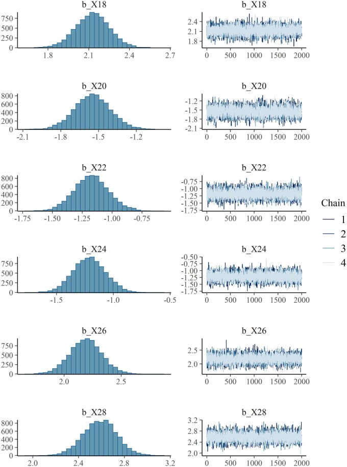 Figure 1
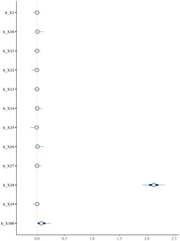 Figure 2
|
| ||||
|
|
|
|
| |
|
|
|
|
|
|
|
|
|
|
|
|
|
|
|
|
|
|
|
|
|
|
|
|
|
|
|
|
|
|
|
|
|
|
|
|
|
|
|
|
|
|
|
|
|
|
|
|
|
|
|
|
|
|
|
|
|
|
|
|
Peer Reviews
No public reviews on file for this paper yet. If you reviewed it on a platform where reviews are public (OpenReview, ICLR, NeurIPS, ICML), you can paste yours below so the community can read it here.
Videos
No videos yet. Explain this paper in a talk, walkthrough, or lecture? Add one.
Taxonomy
TopicsGeochemistry and Geologic Mapping · Gut microbiota and health · Oral microbiology and periodontitis research
1 Introduction
Recent advances in sequencing technologies and computational tools—such as 16S rRNA gene sequencing and taxonomic profiling—have enabled high-throughput characterization of the human microbiome (Jovel et al. 2016, Johnson et al. 2019). These developments have led to the generation of microbiome data summarized as operational taxonomic units (OTUs) (Huse et al. 2012). It facilities researchers exploring the relationships between microbiome composition and health outcomes, with growing interest in using microbiome features to predict disease and inform personalized medicine strategies.
However, incorporating microbiome data as covariates in predictive models presents several analytical challenges: (i) microbiome data are compositional, meaning only relative abundances are observed (Gloor et al. 2017). Due to high sparsity and variability in count data, these covariates are typically transformed and analyzed using compositional data analysis techniques; (ii) the hierarchical and correlated structure of microbiome data, embedded within a phylogenetic tree and classified across taxonomic levels, introduces intrinsic relationships among taxa that complicate variable selection and coefficient estimation (Martiny et al. 2015); (iii) the high dimensionality of microbiome data—often involving thousands to tens of thousands of taxa—contrasts sharply with the relatively small number of available samples, necessitating advanced regularization or Bayesian shrinkage approaches (Chen et al. 2013); (iv) modeling disease outcomes is complicated by their diverse forms, including continuous measures, binary indicators, ordinal stages, and time-to-event outcomes, requiring flexible modeling frameworks (Zhang et al. 2024a,b).
Various methods have been proposed to address these challenges. To handle the high dimensionality of microbial features, researchers have employed Bayesian approaches and penalized regression techniques. The compositional nature of microbiome data—has typically been addressed through sum-to-zero constraints on the coefficients (Lin et al. 2014, Shi et al. 2016). To account for the phylogenetic and taxonomic relationships among microbial taxa, structured Bayesian priors have also been developed (Zhang et al. 2021, 2024a,b). While initial methods focused on continuous outcomes, some have been extended to binary responses (Lu et al. 2019). In our recent work (Zhang et al. 2024a), we further advanced this line of research by developing models capable of handling ordinal outcomes through a Bayesian framework using Markov Chain Monte Carlo (MCMC) algorithms.
Despite these methodological developments, few R packages are currently available to implement such models for compositional microbiome data. The Compack package implements the penalized log-contrast model proposed by Lin et al. (2014) for continuous outcomes. The coda4microbiome package, developed by Calle and Susin, applies elastic-net penalization to all possible pairwise log-ratios in generalized linear models (GLMs), supporting continuous and binary outcomes(Calle and Susin 2022). Additionally, the bglm function in the BhGLM package enables Bayesian hierarchical modeling, including applications to compositional data(Yi et al. 2019, Zhang et al. 2025a).
However, these packages are limited in several important ways. All are restricted to either binary or continuous outcomes, with Compack only applicable to continuous data. Moreover, both Compack and coda4microbiome rely on penalization-based regression approaches that yield point estimates and do not provide full posterior distributions, thus failing to capture uncertainty in parameter estimates and predictions. Crucially, none of these packages incorporate phylogenetic relationships among microbial taxa, which are essential for accurately modeling the inherent structure of microbiome data.
A flexible and efficient R package is essential for advancing the analysis of compositional microbiome data in disease research. We present BCGLMs, a freely available R package designed to predict disease outcomes using compositional microbiome predictors, based on our previously published methods. The package implements four Bayesian modeling approaches: BCGLM, BCO, BCCOXPH, and BCGLMM. In our prior work, we evaluated against existing tools and demonstrated that BCGLM outperforms the popular functions in packages such as Compack and coda4microbiome, yielding more accurate coefficient estimates and lower prediction error in compositional data analysis (Zhang et al. 2024b). The BCO method is the first and only approach developed to handle multi-level ordinal responses using compositional microbiome data (Zhang et al. 2024a). The BCGLMM method introduces additional innovation by incorporating random effects, allowing for the detection of both moderate effects from specific taxa and the cumulative influence of many low-abundance taxa (Zhang et al. 2025b). Together, these tools make BCGLMs a comprehensive and practical solution for microbiome-based disease modeling.
2 Models and algorithms
Assume we collected microbiome samples. For each sample, we observe a response variable and m compositional microbiome taxa, represented as relative abundance tax—i.e. the observed counts divided by the total sequences. Let denote the resulting matrix of microbiome covariates, with ( ) and for all i. The response may be continuous, binary, ordinal or survival. We link the response to the microbiome covariates, using an appropriate link function depending on the response type. To account for the compositional nature of the microbiome covariates, we use log-contrast models with sum-to-zero constraint (Lin et al. 2014, Shi et al. 2016, Lu et al. 2019):
In generalized linear models, is linked to the response y through a link function :
For survival outcome, we consider the Cox proportional hazards model, where the hazard function of the survival time is modeled as:
This sum-to-zero constraint ensures identifiability and reflects the compositional nature of the data. In Bayesian framework, this constraint can be softly enforced by assigning a prior (Zhang et al. 2024a,b, 2025a,b):
which we refer to as “soft-centering”. This approach allows for implementation within the brms package in R, which provides a flexible interface for Bayesian modeling using Stan (Gelman et al. 2015). The brms framework enables user-defined priors and automatically compiles the corresponding Stan code, facilitating model specification and estimation (Bürkner 2017).
To account for phylogenetic and taxonomic relationships between taxa and incorporate this relation in variable coefficients estimation, we use regularized horseshoe priors on compositional covariates coefficients(Piironen and Vehtari 2017):
the regularized horseshoe is a continuous shrinkage prior that includes both a global scale parameter , and the local shrinkage parameters for each . The global parameter controls overall shrinkage across all taxa, while the local parameters allow for coefficient-specific regularization. This structure enables the model to apply strong shrinkage to irrelevant taxa while preserving signals with substantial effects, thereby improving estimation accuracy in high-dimensional settings.
We incorporate phylogenetic structure by modeling the local shrinkage parameters based on a taxon-level similarity matrix (Randolph et al. 2018), constructed from a phylogenetic square distance matrix D^(2)^ (Randolph et al. 2018):
This structure is modeled using an intrinsic autoregressive (IAR) prior (Morris et al. 2019), which induces correlated shrinkage across phylogenetically related taxa. This hierarchical structure can also be implemented via brms through custom prior specification.
In the BCGLMM model, we further introduce a sample-level random effect to capture the cumulative small effects (Zhang et al. 2025b),
where is a sample-level similarity matrix constructed to encode relationships among samples, such as shared environmental or clinical features (Zhao et al. 2015).
The model is estimated using the Hamiltonian Monte Carlo (HMC) algorithm and its adaptive variant, the No-U-Turn Sampler (NUTS), in Stan (Gelman et al. 2014). These MCMC methods efficiently generate posterior samples from the joint distribution defined by the likelihood and the prior specifications. The resulting posterior draws are used to summarize the distribution of each model parameter, enabling both point and interval estimation, and supporting inference on effect sizes and prediction accuracy.
3 Features
In the developed R package, we provide four core functions: bcglm, bco, bccoxph, and bcglmm, which implement compositional generalized linear models (GLMs), compositional cumulative logistic regression, compositional survival CoxPH regression, and compositional GLM mixed models, respectively. For bcglm, bco, and bccoxph, incorporating a similarity matrix between taxa is optional. To facilitate this, we include a similarity function that computes the similarity matrix based on phylogenetic or taxonomic information. Users can choose whether to include this matrix in the model; by default, the similarity matrix is not used, meaning the phylogenetic relationships among taxa are ignored.
To support model implementation, the package also provides simulation functions for each model type. The functions sim_c and sim_b generate simulated microbiome covariates under a compositional framework for continuous and binary response, respectively, as described in our paper (Zhang et al. 2024b). The sim_s function generates simulated compositional variables for survival responses. The sim_o function generates simulated compositional variables for ordinal responses (Zhang et al. 2024a), and sim_cmm simulates compositional variables with a mixture of both large and small effect sizes, where the proportion of small effects can be specified relative to the total number of predictors (Zhang et al. 2025b).
The BCGLMs package uses brms as the underlying Bayesian regression engine for model fitting. Therefore, summary and diagnostic tools provided by brms—such as summary(), fixef(), and plot()—remain fully available to users. These functions allow users to extract posterior summaries (e.g. means, standard errors, and 95% credible intervals for regression coefficients) and to generate standard diagnostic figures, including trace plots and posterior density plots. The mcmc_plot() function, implemented in bayesplot and accessible through brms, provides additional visualization of posterior estimates and uncertainty.
4 Results
In our published work introducing the bcglm, bco, and bcglmm methods, we conducted simulation studies to evaluate the performance of each approach. In this section, we demonstrate how to apply each method using the corresponding simulation functions provided in the package. These functions ultimately call the brm function from the brms package, with the regularized horseshoe prior incorporated for coefficient estimation. In the work (Zhang et al. 2024a,b), we have shown that the global shrinkage parameter with a heavy-tailed Cauchy prior is minimally impacted by the choice of the scale ; in this article, we use the default setting with a scale of 1.
To use the BCGLMs package, users can install it from GitHub. The package depends on several R packages, including phyloseq, BhGLM, and brms. For users running R version 4.4.x, the following code can be used to install the required packages and BCGLMs:
#Install dependencyif (! require(“BiocManager”, quietly = TRUE)) { install.packages(“BiocManager”)}BiocManager::install(“phyloseq”)install.packages(“remotes”)remotes::install_github(“paul-buerkner/brms”)remotes::install_github(“nyiuab/BhGLM”, force = TRUE)Note:Please check Bioconductor—phyloseq for more versions of phyloseq.BhGLM is currently compatible with R ≤ 4.4.x. Users running R ≥ 4.5 may encounter installation or runtime errors because the package has not been updated for recent R versions.#Install BCGLMsremotes::install_github(“Li-Zhang28/BCGLMs”, force = TRUE, build_vignettes = TRUE)
Here, we demonstrate the use of bcglm to analyze example data.
4.1 Demonstration of bcglm using simulated data
The bcglm function is designed to analyze compositional microbiome data with either continuous or binary outcomes. The simulation functions sim_c and sim_b generate correlated compositional data with continuous and binary responses, respectively, replicating the setup from our paper (Zhang et al. 2024b). Users can specify the sample size and number of taxa (i.e. covariate dimensionality), and the output is a list containing simulated compositional predictors and outcomes.
After generating the data, users can fit the model using bcglm, with the option to include a taxon-level similarity matrix. We also provide a similarity function to compute this matrix based on phylogenetic or taxonomic information. The inclusion of this similarity structure allows the model to account for phylogenetic relationships among taxa during estimation.
In this simulation, we generated 100 compositional variables and a continuous response for 400 samples. The similarity matrix was calculated and stored as sim, which was then incorporated into the model fitting using the bcglm function. The parameters df_local and df_global specify the degrees of freedom for the Student-t distributions on the prior of local shrinkage parameters and the global shrinkage parameter in the regularized horseshoe prior. By default, both parameters are set to 1, corresponding to a half-Cauchy distribution. Users may also define half-t priors with smaller degrees of freedom to induce heavier tails and allow for more flexible shrinkage behavior.
dat = sim_c( * n * = 400, p = 100) otu=otu_table(dat$x, taxa_are_rows = F)
dis.taxa = phyloseq::distance(otu, method = “bray”, type = “taxa”)
sim
similarity(dis.taxa)
fit = bcglm(x = daty, family = gaussian, df_local = 1, df_global = 1, similarity = sim)
After model fitting, posterior summaries—including the point estimates and the 2.5% and 97.5% quantiles—can be extracted for the regression coefficients.
**: **
We can also examine trace plots and density plots (Fig. 1) using the plot function for specific variables.
Density and trace plots of selected non-zero effects from the simulation.
plot (fit, variable = c(“b_X18”, “b_X20”, “b_X22”, “b_X24”, “b_X26”, “b_X28”), nvariables = 6)
Additionally, the mcmc_plot function can be used to visualize posterior draws for selected parameters. For example, we can display the credible intervals for variables that start with X1 (Fig. 2).
mcmc_plot(fit, variable = “^b_X1”, regex = TRUE)
Posterior mean and 95% credible interval from MCMC draw for selected effects.
In this example, we incorporate phylogenetic relationships by including a similarity matrix. Users may also set the similarity argument to NULL to ignore the relationships between taxa. The function sim_b can be used in a similar manner to generate a binary response, and model fitting is achieved by setting the family argument to Bernoulli in the bcglm function.
The simulation utilities included in BCGLMs are simple demonstration tools, designed to illustrate the basic workflow of Bayesian compositional generalized linear models rather than providing a fully flexible or highly customizable simulation framework. Several parameters in these functions are intentionally fixed or limited to ensure reproducibility and ease of use. Users can leverage these examples to explore model fitting, posterior summaries, and diagnostic plots; however, the functions are not intended for extensive simulation studies or advanced parameter exploration. Users may extend these functions to explore additional simulation scenarios as needed.
5 Conclusions
We have developed a freely available R package, BCGLMs, to address the analytical challenges associated with compositional microbiome variables and different types of outcomes. Although built on the brms package, BCGLMs extends its functionality in several keyways to enhance usability, integration, and accessibility. First, it directly models covariates on the simplex, which is appropriate for microbiome relative abundance data. Second, it implements a structured version of the regularized horseshoe prior, enabling adaptive and interpretable shrinkage for high-dimensional compositional features. Third, BCGLMs allows the incorporation of phylogenetic relationships among taxa via prior specification, providing more biologically informed modeling. Together, these features offer a streamlined workflow for compositional microbiome data analysis, reducing the need for complex preprocessing or manual model specification. In addition, BCGLMs improves accessibility by packaging advanced Bayesian methods into a user-friendly interface, lowering the expertise required to apply these models in practice.
BCGLMs incorporate phylogenetic relationships using kernel-based similarity matrices, but its primary focus remains on directly modeling the compositional structure of microbiome data. In contrast to many kernel- or distance-based approaches, BCGLMs employs a fully Bayesian MCMC framework, providing posterior distributions for regression parameters rather than only point estimates (Zhang et al. 2024a,b). This allows for richer inference, including uncertainty quantification and interpretable shrinkage, which is particularly valuable when analyzing high-dimensional compositional features with complex dependencies.
Although primarily designed for microbiome studies, the Bayesian modeling framework underlying BCGLMs is broadly applicable to a wide range of compositional data contexts. With its extensible design and scalability, the package provides a versatile toolkit for researchers working with both standard and large-scale compositional datasets.
The reference list from the paper itself. Each links out to its DOI / PubMed record.
- 1Bürkner P-C. brms: an R package for Bayesian multilevel models using stan. J Stat Soft 2017;80:1–28.
- 2Calle ML, Pujolassos M, Susin A. coda 4microbiome: compositional data analysis for microbiome cross-sectional and longitudinal studies. BMC Bioinformatics 2023;24:82. 10.1186/s 12859-023-05205-3 · doi ↗
- 3Chen J , Bushman FD, Lewis JD et al Structure-constrained sparse canonical correlation analysis with an application to microbiome data analysis. Biostatistics 2013;14:244–58.23074263 10.1093/biostatistics/kxs 038PMC 3590923 · doi ↗ · pubmed ↗
- 4Gelman A , Carlin JB, Stern HS et al Bayesian Data Analysis. Boca Raton: Chapman and Hall/CRC, 2014.
- 5Gelman A , Lee D, Guo J. Stan: a probabilistic programming language for Bayesian inference and optimization. J Educ Behav Stat 2015;40:530–43.
- 6Gloor GB , Macklaim JM, Pawlowsky-Glahn V et al Microbiome datasets are compositional: and this is not optional. Front Microbiol 2017;8:2224.29187837 10.3389/fmicb.2017.02224 PMC 5695134 · doi ↗ · pubmed ↗
- 7Huse SM , Ye Y, Zhou Y et al A core human microbiome as viewed through 16S r RNA sequence clusters. P Lo S One 2012;7:e 34242.22719824 10.1371/journal.pone.0034242 PMC 3374614 · doi ↗ · pubmed ↗
- 8Johnson JS , Spakowicz DJ, Hong B-Y et al Evaluation of 16S r RNA gene sequencing for species and strain-level microbiome analysis. Nat Commun 2019;10:5029.31695033 10.1038/s 41467-019-13036-1PMC 6834636 · doi ↗ · pubmed ↗