Evidence accumulation from experience and observation in the cingulate cortex
Ruidong Chen, Setayesh Radkani, Neelima Valluru, Seng Bum Michael Yoo, Mehrdad Jazayeri

TL;DR
This study shows how the brain combines personal experience and observation to update beliefs in a social setting.
Contribution
It identifies the anterior cingulate cortex as the brain region integrating experiential and observational evidence.
Findings
Humans and monkeys updated beliefs effectively through experience but less so through observation.
Anterior cingulate cortex integrates experiential and observational evidence into a coherent belief representation.
Population activity geometry reveals the computational architecture of evidence integration.
Abstract
We use our experiences to form and update beliefs about the hidden states of the world1–3. When possible, we also gather evidence by observing others. However, how the brain integrates experiential and observational evidence is not understood. We studied the dynamics of evidence integration in a two-player game with volatile hidden states. Both humans and monkeys successfully updated their beliefs while playing the game and observing their partner, though less effectively when observing. Electrophysiological recordings in animals revealed that the anterior cingulate cortex integrates independent sources of experiential and observational evidence into a coherent neural representation of dynamic belief about the environment’s state. The geometry of population activity revealed the computational architecture of this integration and provided a neural account of the behavioral asymmetry…
Genes, proteins, chemicals, diseases, species, mutations and cell lines named across the full text — each resolved to its canonical identifier and authoritative record.
Click any figure to enlarge with its caption.
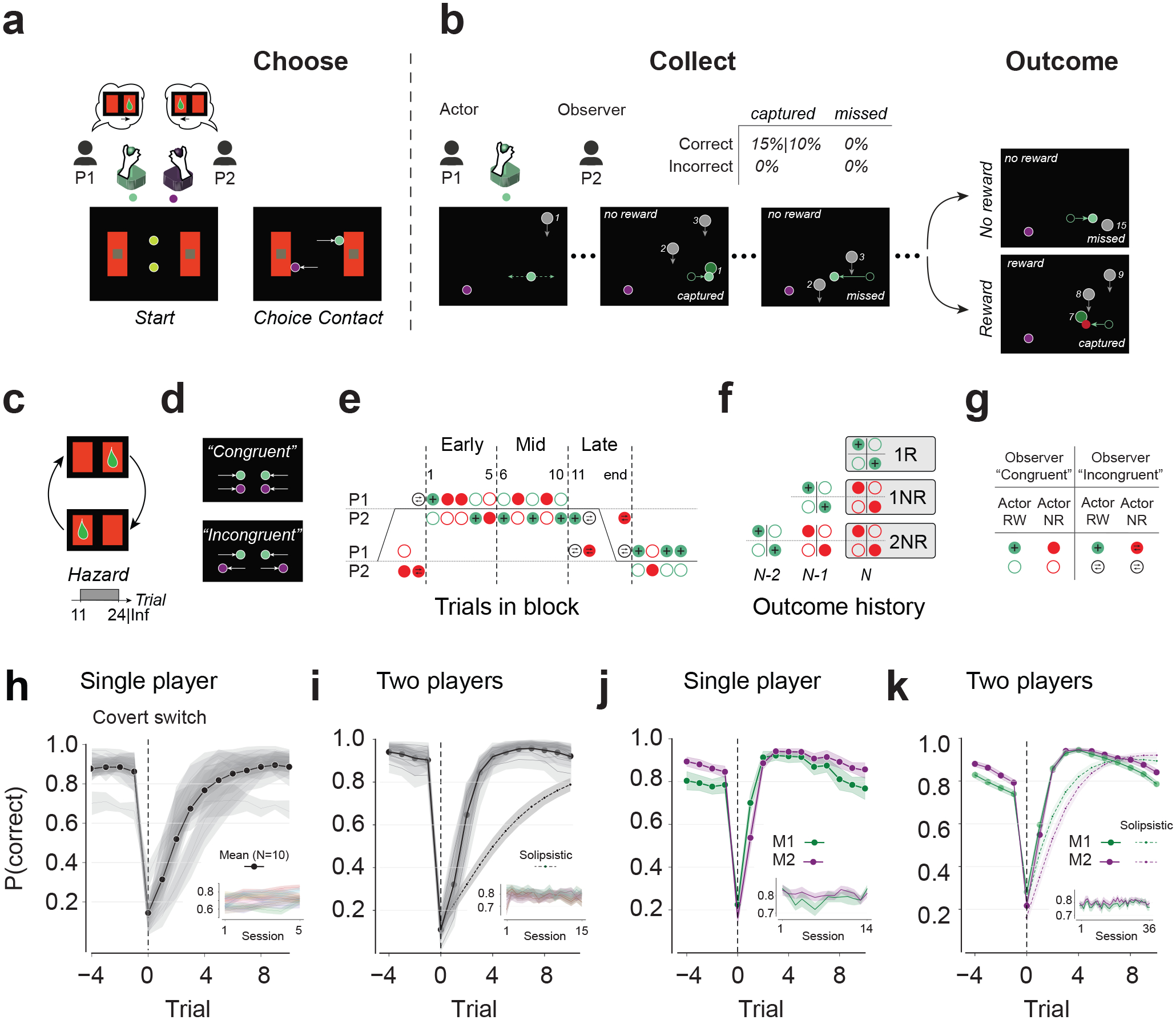 Figure 1
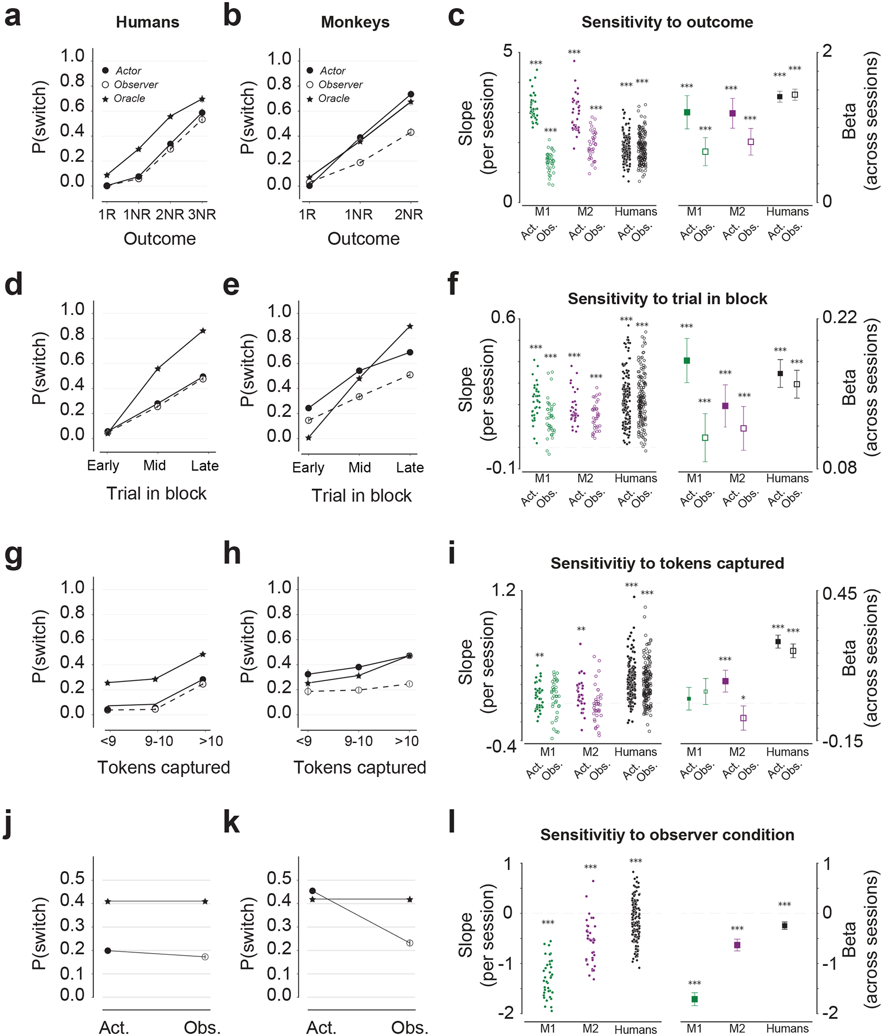 Figure 2
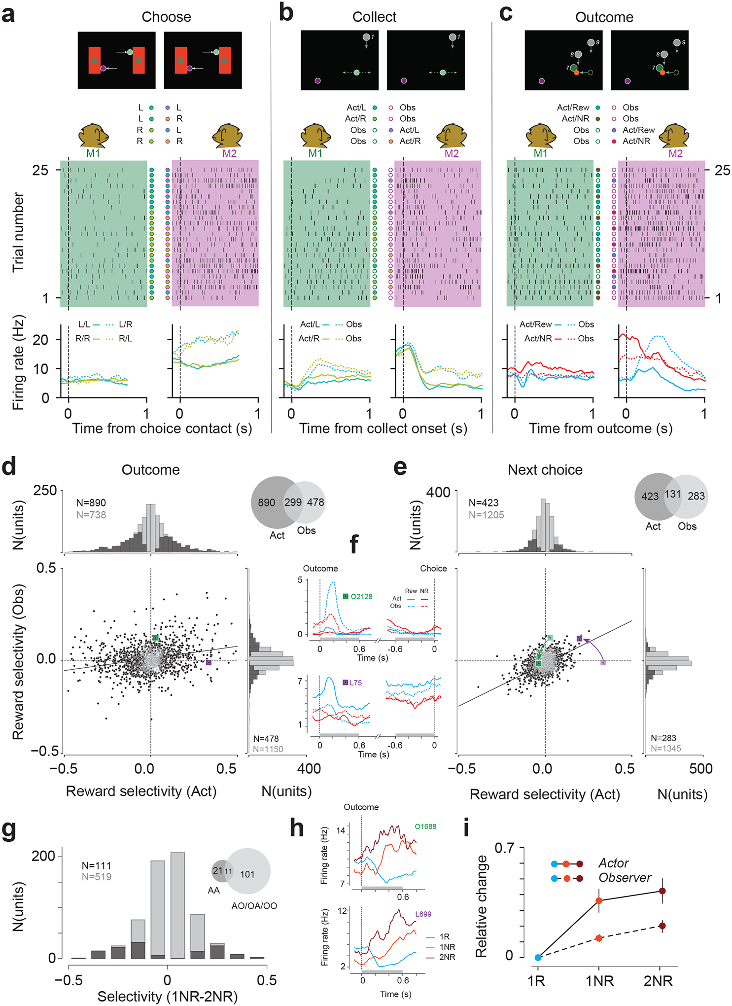 Figure 3
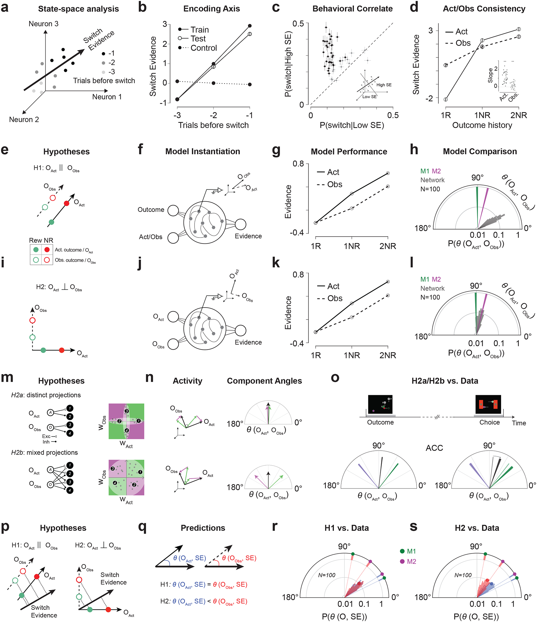 Figure 4
Peer Reviews
No public reviews on file for this paper yet. If you reviewed it on a platform where reviews are public (OpenReview, ICLR, NeurIPS, ICML), you can paste yours below so the community can read it here.
Videos
No videos yet. Explain this paper in a talk, walkthrough, or lecture? Add one.
Taxonomy
TopicsAction Observation and Synchronization · Face Recognition and Perception · Embodied and Extended Cognition
A hallmark of cognition is the ability to infer the hidden causes of our experiences. Waking up with an upset stomach, you might wonder if it is due to food poisoning or if you caught the flu. Your first clues are your symptoms—nausea versus fever would hint at different causes. But you may also rely on others’ experiences. You may think it is flu if a coworker recently had the flu, or you may reason it is food poisoning if your dinner partner has similar symptoms. While the capacity to integrate experiential and observational evidence to infer hidden causes is unequivocal, the neural mechanisms that enable such sophisticated computations are not well understood.
The anterior cingulate cortex (ACC) is thought to play a central role in evidence-based decision making. ACC carries signals related to outcome history, performance monitoring, action and strategy selection, and beliefs about associations and contexts^1–21^. Notably, ACC representations persist over relatively long time scales^22^ and integrate information across events and experiences^1–3,23^. These findings coupled with complementary causal studies^3,15,24–26^ have provided strong evidence that ACC encodes behaviorally-relevant beliefs about latent causes in the environment.
We know far less about the computational and neural basis of observational inference and learning. Some studies have examined the neural signatures of observed reward and punishment^27^ in the amygdala, striatum, and many cortical areas^28–39^. Among these, ACC has been a prominent region of interest that supports vicarious reinforcement and observational fear conditioning^33,35,36,39–42^. Therefore, ACC may play a more general role in belief updating that spans both experiential and observational settings.
However, most studies on observational learning have relied on relatively simple tasks that either do not require inferring latent causes or do not involve integration of experiential and observational evidence. As a result, little is known about the parallels and distinctions between the neural representation of experiential and observational evidence, and how these two sources of information are integrated to form beliefs about the latent state of the world.
Here, we tackle these questions using a combination of human behavior, primate neurophysiology, and neural modeling in a two-player belief-updating game. The behavioral results revealed a familiar asymmetry between experiential and observational evidence^43–45^ in both humans and monkeys. ACC recordings revealed how the evidence derived from self and other experiences are integrated into a coherent population pattern of neural activity supporting participants’ beliefs and behavior on a trial-by-trial basis. Moreover, the organization of the population activity associated with self-experience, observation, and integrated belief provided an explanation for the behavioral asymmetry.
Behavioral task and performance
We designed a two-player game for humans and monkeys to investigate the behavioral and neural signatures of updating beliefs in the presence of both experiential and observational evidence (Figure 1a–g). Each trial consists of two phases. In the first phase, the players use their respective joysticks to independently choose between a left and a right arena (Figure 1a). They are free to choose either arena (Figure 1d) but this choice is consequential because only one of the arenas may eventually lead to a reward (Figure 1c). Human participants additionally reported their choice confidence (see Methods).
In the second phase, one player is randomly designated as the actor. The actor controls an avatar in their chosen arena with the joystick and must capture tokens falling from the top of the screen, aiming to collect as many as possible to maximize expected reward. Receiving reward is probabilistic and depends on both the arena and the number of captured tokens during the second phase (Figure 1b). If the actor selects the correct arena, each captured token has a fixed probability of yielding a reward (0.1 for humans and 0.15 for monkeys), and the delivery of reward would terminate the trial (i.e., no more token capture allowed). In the other arena, capturing tokens never results in a reward. Trials without rewards end after all 15 tokens have dropped. The correct arena switches in a blocked fashion (Figure 1c). From the moment the actor begins to collect tokens to the end of the trial, the other player, whom we refer to as the observer, watches the actor play and witnesses the outcome without receiving any reward.
We matched the actor’s and observer’s sensory experiences as closely as possible: both saw all events, the actor was designated only after both chose an arena, and roles were assigned randomly. Thus, both had equal information for rational inference, ensuring any asymmetries in evidence accumulation reflect internal rather than external factors.
We collected data from ten humans (five pairs) and two monkeys. All participants learned the task in a single-player version (average choice performance (mean±SD) in humans: 71.85±7.02% across 5 sessions, Figure 1h; in M1: 78.39±3.34% and in M2: 80.96±1.65% across 14 sessions, Figure 1j) before moving onto the two-player version (performance in humans 79.15±3.05% over 15 sessions, Figure 1i; in M1 78.68±2.07%, and M2 80.38±1.73% over 36 sessions, Figure 1k). Monkeys trained longer and faced higher reward probabilities. In both versions, performance dropped immediately after covert block switches and recovered within a few trials, indicating belief updating (Figure 1h–k, S2c–f). We used single-player data to simulate “solipsistic” agents that ignored observer trials (see Methods). As expected, solipsistic agents performed worse than their respective single-player source due to ignored observer trials (humans: 50.72±10.90%; M1: 74.82±3.27%; M2: 71.40±3.09%), and significantly worse compared to the two-player sessions (Figure 1i,k). Attention to observer trials was evident in monkeys’ eye movement data, with preferential orienting of gaze toward the active arena (M1: 58.0 ± 22.5%; M2: 87.4 ± 18.7%; Figure S1h,k).
Humans and monkeys integrate experiential and observational evidence rationally
To evaluate the degree to which participants played the game rationally, we compared their behavior to that of an optimal “oracle” model (Figure 2). Specifically, we analyzed the decision to switch on the next trial as a function of three factors: (1) history of trial outcomes (including the current trial), (2) position of the current trial in the block, and (3) number of captured tokens in the current trial. To ensure a fair comparison between actor and observer, we first focus on congruent trials where both players chose the same arena.
Behavioral consequences of outcome history (Figure 2a–c).
Because only one arena yields rewards, the oracle treats rewarded trials as confirmation of a correct choice and consecutive no reward trials as accumulating evidence for a switch (star, Figure 2a,b). The choice behavior of both humans and monkeys showed a similar pattern: Switch probability, denoted P(switch), was low after rewarded trials and increased monotonically with consecutive unrewarded trials (Figure 2a–b, S4a–b). This pattern was evident in single sessions (Figure 2c, left), remained significant in a logistic regression analysis that accounted for outcome history, trial in block, and number of captured tokens (Figure 2c, right), and was corroborated by the pattern of human confidence reports (Figure S3a).
Behavioral consequences of trial position in the block (Figure 2d–f).
Since switches are less likely early on compared to later in the block, the oracle is more likely to switch later in the block (star, Figure 2d,e). As neither the oracle nor the participants were aware of block switches, we inferred subjective block switches from the behavior (Figure S2e–f) and registered trial position within subjective blocks (see Methods). In accordance with the oracle, P(switch) for both humans and monkeys increased monotonically with trial position in the block (Figure 2d–e, S4c–d). This effect was evident in single sessions (Figure 2f, left), remained significant in a multivariate logistic regression analysis (Figure 2f, right), and was corroborated by the pattern of human confidence reports (Figure S3a).
Behavioral consequences of number of captured tokens (Figure 2g–i).
The probability of success increases with the number of captured tokens. Participants understood this contingency and aimed to maximize the number of captured tokens (see Methods; Figure S2g–h). Moreover, as predicted from the oracle (star, Figure 2g–h), participants must treat unrewarded trials with larger numbers of captured tokens as stronger evidence for a block switch. Qualitatively, this effect was evident in human participants’ behavior (Figure 2g, S3a), and to a lesser degree in monkeys (filled, Figure 2h, S4e–f). However, a more rigorous multiple regression analysis indicated that the effect was significant only in humans, and in Actor condition for one of the animals (Figure 2i, S3b).
Behavioral consequences of the choice incongruence (Figure S5).
We also analyzed incongruent trials where participants chose opposite arenas. These trials were more frequent later in the block (Figure S5a,d), as expected by the higher switch probability, and were associated with lower confidence reports in humans (Figure S5c). Moreover, across human participants and one monkey, the actor was more likely to switch following incongruent trials (Figure S5b,e–g), indicating that players were influenced by each other’s decisions on top of their experiences and outcomes.
Humans and monkeys discount observational evidence
By design, the oracle evaluates actor and observer trial outcomes identically (star, Figure 2j–k). In contrast, humans and monkeys weighted observational evidence less than experienced evidence (Figure 2j–k) even though actor and observer were randomly assigned and had identical visual experiences. This asymmetry was stronger in monkeys, possibly because the actor monkey received juice reward. Notably, the asymmetry was evident in single sessions (Figure 2l, left), and remained significant after accounting for other experimental factors (Figure 2l, right). This result indicates that humans and monkeys were less responsive to unrewarded trials as an observer. Notably, this asymmetry was not due to players spending less time looking at the screen when designated as observer (Figure S1e–m). This asymmetry was also reflected in humans’ confidence reports when they chose to stay in the same arena (Figure S3a).
Experiential and observational evidence integration in the cingulate cortex
Our behavioral results provided compelling evidence that monkeys, like humans, integrate experiential and observational evidence to infer latent state switches. To investigate the underlying neural computations, we recorded neural activity in ACC (see Table S1 for stereotaxic coordinates) simultaneously from the two animals.
Our recordings (M1: 31 sessions; M2: 20 sessions; simultaneous recording in 19 sessions) yielded 1628 units (M1: 859; M2: 769). Most task-modulated neurons were sensitive to multiple variables and their sensitivity could change throughout the trial (Figure 3a–c). For example, we found mixed selectivity to trial outcome for the actor and observer (Figure 3d,e,S6a–d) with a large proportion sensitive to actor outcome (bootstrap test, p<0.05 in 890/1628=54.7% of all neurons in both animals, see Methods), a smaller proportion to observer outcome (bootstrap test, p<0.05 in 478/1628=29.4% of all neurons in both animals), and a sizeable overlap between the two (299/1069=28.0% of outcome selective neurons). Moreover, this sensitivity changed throughout the trial, as evident from single neurons (Figure 3f) and across the population (Figure 3d–e, regression slopes). Notably, the alignment for outcome encoding between the actor and observer increased in the choice phase compared to the outcome phase (Figure 3d–e; regression slope in choice: 0.46±0.03; outcome: 0.13±0.01; variance explained in choice: 32%; outcome: 6%). This result is consistent with a gradual integration of distinct actor- and observer-dependent responses into an identity-agnostic outcome representation.
We further analyzed single neurons for evidence of outcome integration across actor and observer trials. Integration requires firing rate modulations for the actor and observer to be in the same direction; opposite directions would counter integration. Accordingly, we restricted our analysis to 630 neurons with same-sign outcome selectivity for actor and observer (Figure 3d–e, 1^st^ and ^3rd^ quadrants) and quantified the difference between firing rates in the 1NR and 2NR conditions (Figure 3g, S6e,f). Across this population, 17.6% (111/630) were more strongly modulated for 2NR compared to 1NR trials. This effect was also evident in the average firing rates of individual neurons (Figure 3h).
Previous work has shown that ACC neurons integrate cross-trial evidence in single-player tasks that involve only experiential evidence^3,10,23^. As such, it is critical to subdivide 2NR trials and distinguish between Actor-Actor trials that involve only experiential evidence and the other three conditions that have at least one observer trial (Actor-Observer, Observer-Actor, and Observer-Observer). Doing so, we found that 91.0% (101/111) of neurons that featured evidence accumulation were sensitive to observer trials (Figure 3g, inset).
A notable feature of behavior was the asymmetry in evidence accumulation: unrewarded trials, matched in every other aspect, were weighed more strongly in actor trials compared to observer trials. We therefore asked whether firing rate changes in neurons featuring evidence accumulation were also stronger for actor trials. Indeed, firing rate modulations in the 1NR and 2NR trials compared to rewarded trials were stronger in the Actor condition (Figure 3i, S6h–i, mean z-scored rate change in actor condition: 0.36 in 1NR, 0.42 in 2NR; observer condition: 0.12 in 1NR, 0.20 in 2NR; p<0.001 between Actor and Observer conditions, paired t-tests).
The neural geometry of multi-agent evidence accumulation
While single neurons encoded a wide range of task variables, this sensitivity was typically mixed, changing both during the trial (Choose versus Collect versus Outcome phases) and as a function of trial type (e.g., Actor versus Observer). This property, which is common across frontal cortical neurons^46^, motivated further neural analysis at the population level, which can offer complementary computational insights^47–49^.
A stable dimension encoding switch belief (Figure 4a–d).
First, we identified a dimension along which activity increased monotonically across trials leading to a behavioral switch (Figure 4a, see Methods). Using cross-validation, we verified that this dimension predicted switch behavior (Figure 4b; Figure S7a–b for individual animals). Importantly, this effect was specific to trials preceding switches and was not due to a trial-order effect (Figure 4b, dashed). We also confirmed the link between the encoding dimension and switch behavior by verifying that large and small projections of neural activity on the encoding dimension corresponded to high and low values of P(switch), respectively (Figure 4c).
Because behavior was influenced by both Actor and Observer trials, we examined projections onto the encoding dimension for each trial type separately. This dimension carried outcome information for both, with larger projections in 2NR than 1NR trials (p < 0.001 in both Actor and Observer conditions, paired t-tests; Figure 4d; Figure S7e–f for individual animals). This observation was evident within sessions as quantified by the regression slopes relating projections to the number of unrewarded trials (Figure 4d, inset). Consistent with behavioral asymmetry, regression slopes were steeper for Actor than Observer trials (p < 0.001, paired t-test, Figure 4d, inset). Control analyses confirmed that this difference was not explained by unequal trial counts or neuron numbers (Figure S11a–c).
Identity and outcome inputs to ACC (Figure 4e–l).
We examined the neural state space to characterize how inputs to ACC convey information about identity and outcome. We considered two hypotheses. H1 proposes a shared, identity-agnostic input for outcomes and a separate input for identity. This arrangement yields parallel encoding dimensions for Actor and Observer outcomes (Figure 4e). H2, in contrast, posits independent inputs for experienced and observed outcomes, producing orthogonal encoding dimensions (Figure 4i).
To test these hypotheses, we compared the geometry of ACC population activity with that of recurrent neural network (RNN) models implementing each hypothesis. In H1, the RNN received one input conveying identity-agnostic outcome information and another signaling identity (Figure 4f). In H2, it received separate inputs for experienced and observed outcomes (Figure 4j). We trained 100 randomly initialized RNNs per hypothesis (see Methods).
All RNNs successfully integrated evidence and reproduced the behavioral asymmetry (Figure 4g,k; Figure S8). We then compared their outcome representational geometry to that of ACC, identifying Actor and Observer encoding dimensions in each dataset and evaluating H1 and H2 based on the angle between these dimensions in the models and ACC.
We compared RNNs instantiating H1 and H2. The angle between Actor and Observer dimensions was smaller and closer to parallel in H1 (30.77 ± 6.88°, mean ± SD, N = 100; Figure 4h) and larger, approaching orthogonality, in H2 (78.89 ± 7.56°, N = 100; Figure 4l). ACC data showed similarly large angles (M1: 90.83 ± 1.35°; M2: 75.97 ± 1.28°; N = 100 splits per animal), consistent with H2 predictions (Figure 4h,l). This orthogonality was not explained by firing rate differences in rewarded trials: differences during unrewarded trials were equally strong and frequent (rewarded: n=375/1628, p<0.05, average z-scored rate difference=0.31; unrewarded: n=358/1628, average z-scored rate difference=0.34; Figure S12c). Moreover, orthogonality persisted when considering only unrewarded trials (Figure S12f).
To test whether the independent inputs are necessary for orthogonality, we trained additional RNNs with the H1 input architecture but imposed a constraint enforcing a large angle between the Actor and Observer outcome dimensions. These models failed to perform the task (Figure S13). These findings strengthen the hypothesis that ACC receives Actor and Observer outcome information via independent input pathways.
Input projection patterns onto ACC (Figure 4m–o, S9a–c).
We analyzed population responses in ACC to dissect the organization of input projections onto ACC. Our previous analysis indicated that ACC receives independent inputs associated with actor and observer outcomes. This orthogonality is consistent with two hypotheses, denoted H2a and H2b. H2a posits that the actor and observer inputs project to disjoint ACC subpopulations (Figure 4m, S9a). This organization is consistent with the input orthogonality because disjoint populations are inherently orthogonal. H2b, in contrast, posits mixed projections to the same population in ACC (Figure 4m, S9a), which could also result in orthogonality.
Many neurons were sensitive to both actor and observer outcomes (Figure 3d, S6a–b). This result provides evidence for some level of mixed projection. To distinguish between H2a and H2b more definitively, we divided the neurons into two groups. The first group, which we refer to as aligned, include neurons whose firing rates move in the same direction for actor and observer conditions, either positively or negatively (Figure 4m, S9a green). The second group, which we refer to as anti-aligned are the neurons that encode outcome with opposite signs (Figure 4m, S9a magenta).
Critically, H2a and H2b make distinct predictions about the geometry of activity within the subspaces formed by these groups. In H2a, where projections are disjoint, the angles between actor and observer outcome representations remain orthogonal for both aligned and anti-aligned neurons (Figure 4n, S9b–c). In contrast, H2b predicts a divergence in the angle relationships: for aligned neurons, the encoding dimensions are more aligned, resulting in acute angles, whereas for anti-aligned neurons, the encoding dimensions are oppositely oriented, leading to obtuse angles (Figure 4n, S9b–c).
In ACC, at the time of outcome, the decomposed angle between actor and observer dimensions had large positive and negative components, consistent with H2b – not H2a (Figure 4o; Figure S7g–h for individual animals). As the task proceeds to time of choice for the next trial, the two vectors become more aligned (angle at outcome: 83.46° ± 0.92°, choice: 69.94° ± 1.98°, Figure 4o), consistent with the increased correlation of single neuron selectivities (Figure 3e). Together these results suggest that the actor and observer outcome inputs drive ACC through mixed projection patterns.
Geometry of evidence integration (Figure 4p–s).
For effective integration, the switch evidence dimension should be outside the null space of both actor/observer outcome encoding dimensions. This predicts that the angle between the actor outcome and switch evidence, θ(OAct,SE), as well as the angle between the observer outcome and switch evidence, θ(OObs,SE) must be less than 90 deg. However, the relative geometry of these dimensions differ under the two hypotheses (Figure 4p). Under H1, because the outcome encoding dimensions are parallel, θ(OAct,SE) and θ(OObs,SE) must be the same (Figure 4p). In contrast, under H2, because the outcome encoding dimensions are orthogonal, θ(OAct,SE) and θ(OObs,SE) can assume different values (Figure 4q).
We measured θ(OAct,SE) and θ(OObs,SE) in both the models and ACC (see Methods). The representational geometry in ACC was better captured by H2 (Figure 4r,s). In both ACC and H2-instantiating RNNs, θ(OAct,SE) was smaller than θ(OObs,SE) (RNN_H2_: 43.15±10.22 vs. 59.11±10.89 deg., M1: 26.25±0.88 vs. 79.05±1.42 deg., M2: 31.96±0.94 vs. 54.40±1.35 deg.). This difference was not explained by unequal trial counts or numbers of outcome-responsive neurons and persisted after controlling for both factors (M1: 34.07 ± 1.82 vs. 74.05 ± 2.44 deg., M2: 33.20 ± 1.37 vs. 48.88 ± 1.75 deg. Figure S11d). By contrast, the two angles had similar magnitudes in the H1-instantiating RNNs (44.03 ± 7.35 vs. 43.48 ± 7.80 deg.).
For integration to occur, actor and observer outcomes must drive a common switch evidence dimension. In this respect, the smaller θ(OAct,SE) relative to θ(OObs,SE) may provide a neural explanation of the behavioral asymmetry in experiential versus observational evidence integration. Specifically, if integration occurs by linear projection of activity along the outcome dimension onto the switch evidence dimension, then a smaller angle between the actor outcome and switch evidence dimensions would enable the same strength of evidence collected on actor trials to produce a higher increment in cumulative evidence (Figure 4p).
To further substantiate the relationship between neural geometry and behavioral sensitivity, we computed the outcome-switch angle separately for each session, for both Actor and Observer conditions. Pooling the data across the two animals, we found strong support for our hypothesis: there was a significant negative correlation between behavioral sensitivity and neural angle across sessions (Figure S14a–c).
Additional analyses of these variables for the two animals and the two conditions separately (Figure S14d–i) revealed that the effects were significant for the Actor condition in monkey M1 and the Observer condition in M2 only. Based on this finding, we hypothesized that the two animals were engaged in a leader–follower dynamic with M2 being more strongly influenced by M1 than the other way around, which was borne out of additional behavioral analyses (Figure S14j; also see Figure 2l).
Together, these results suggest that the angles between switch evidence and outcome dimensions in ACC account for the asymmetry in behavioral sensitivity between Actor and Observer conditions.
So far, we configured all RNNs such that their output weights were fixed. To test the effect of this assumption on our findings, we performed control analyses on RNNs built with learnable output weights (Figure S10b,d). The geometry of evidence integration in these readout-learnable networks was different from both the readout-fixed networks and the ACC. Specifically, they exhibited relatively higher alignment between actor and observer outcome dimensions and outcome and evidence dimensions (Figure S10b,d). These results suggest ACC internal dynamics and not its downstream projections are responsible for evidence integration.
Discussion
Our work brings together two important yet traditionally distinct areas of research concerning the role of ACC in cognition. One important function of ACC is to monitor and integrate one’s experience over time to inform strategic decision-making^6,11,17^. This function supports a wide range of mental computations including explore-exploit trade-offs, cost-benefit analysis, conflict monitoring, and causal inference^1–4,19,23,25^. Another function ascribed to ACC is sensitivity to observed reward and punishment enabling vicarious learning^35,36,39–42^. Our work offers a unifying perspective wherein ACC plays a general role in integrating experiential and observational outcomes over flexible timescales to update belief about environmental states. The confluence of these two research directions brings to focus several important questions.
First, what anatomical substrates and circuit motifs enable the integration of information about self and other? We found that ACC encodes all three key computational variables needed for integration: actor outcome, observer outcome, and integrated belief. A comparison of population activity between models and ACC provided evidence that actor and observer outcomes were associated with activity patterns in orthogonal subspaces. This finding suggests that ACC computes beliefs about the state of the environment by integrating outcome information from distinct identity-dependent input streams.
Analysis of the geometry of neural representation is often used to infer computational algorithms. For example, subspace orthogonality is thought to prevent interference and maximize robustness^47,50–52^, and factorized representations are thought to facilitate structural generalization^49,53–57^. In our work, we augmented this analysis with single-neuron tuning properties to dissect the organization of input projections onto ACC. Results indicated that ACC did not rely on disjoint subpopulations for actor and observer information. Instead, actor/observer information was supplied via overlapping projections. We do not know the constraints that determine the organization of these projections. However, in our experiment, this mixing may facilitate the integration process. With disjoint subpopulations, the integration would have to be augmented by a gating mechanism to select the subpopulation that has to be integrated on each trial. In contrast, the mixed representation provides a single subpopulation of outcome-aligned neurons that can be used for integration in all trials.
Our analyses indicated that ACC coding properties changed throughout the inter-trial interval (Figure 4o, S15)^58^. One notable feature was the reduction of the angle between the population vectors encoding the actor and observer outcomes, from the outcome phase to the choice phase in the next trial. This finding is reminiscent of prior work showing high-dimensional firing-rate vectors rapidly decay to a single dimension during the process of decision-making^59^. However, in our work, this process unfolded in the presence of multiple inputs (two agents) and long timescales (across trials), which pose important constraints on the circuits responsible for evidence accumulation in ACC^60.61^.
Second, does the brain process experiential and observational information similarly? In our two-player game, although humans and monkeys integrated experiential and observational outcomes, they learned less from observations. Discounting observational evidence has been reported previously^43–45^. However, several aspects of our study reinforce the view that there is a fundamental asymmetry between learning from experience and observation. By interleaving actor and observer trials while collecting each player’s choice on every trial, we could track both players’ evolving beliefs with precision. This design choice as well as our analysis of congruent and unrewarded trials enabled us to rule out various confounds that could lead to this asymmetry. Finally, we found this asymmetry to be stronger in monkeys, possibly because monkeys received juice reward, which could accentuate the difference between experience and observation. The difference between humans and monkeys may also stem from superior social cognition in humans enabling more effective evaluation and integration of observations.
We identified a neural correlate of this asymmetry in the ACC, where signals encoding actor outcomes were more closely aligned with cumulative switch evidence than those encoding observer outcomes. Validating the functional relevance of this finding will require precise patterned activations of subpopulations of neurons in ACC^62–64^. Additionally, characterizing the behavioral contingencies and neural constraints that give rise to this asymmetry remains an important direction for future research.
In sum, our work establishes the basic mechanisms of multi-agent evidence integration and offers a starting point for addressing exciting and unresolved questions about social learning. Extensions of our work can be used to study the mechanisms through which cognitive factors such as belief about the partner’s skill level, their prior knowledge about task contingencies, and their social rank influence observational learning.
Methods
We collected behavioral data from humans, and behavioral and neurophysiological data from rhesus macaque monkeys (Macaca mulatta). Experimental procedures for humans were approved by the Committee on the Use of Humans as Experimental Subjects at the Massachusetts Institute of Technology. Experimental procedures for animals conformed to the National Institutes of Health guidelines and were approved by the Committee of Animal Care at the Massachusetts Institute of Technology.
Experimental procedures for non-human primates
Two monkeys (M1, female, 6 Kg, aged 6; M2: male, 11 Kg, aged 11) were seated comfortably in two adjacent primate chairs in a dark quiet enclosure at a distance of 40 inches. Animals were head-restained, facing forward, and unable to see one another. Stimuli were presented on two side-by-side display monitors (Acer R240HY) 40 inches apart (center to center), at a normal distance of 19 inches from the animals’ eyes. The monitors displayed identical stimuli throughout experiments. Each animal could manipulate a joystick (Logitech Extreme 3D Pro) placed at a distance adjusted for each animal’s reach (~6 inches) in front of their chair. Joysticks were physically constrained to left/right movements only. The joystick digital output (1–1024) was thresholded to three states: left movement (1–463), no movement (464–560), and right movement (561–1024). Eye movements were sampled at 1kHz using infrared cameras (Eyelink 1000, SR Research). The MWorks software package (http://mworks-project.org) and MOOG library^65^ (https://jazlab.github.io/moog.github.io/) were used to generate visual stimuli and to enforce behavioral contingencies. A photodiode was used to sync electronic events with stimulus presentations.
Neural recordings were made from the anterior cingulate cortex (ACC) with 64-channel linear probes with 50-μm inter-electrode spacing (V-probe, Plexon Inc.) inserted through a rectangular recording chamber. Extracellular signals were bandpass filtered (300 Hz to 6 kHz) and digitized (sampling rate: 30 kHz) using two 32-channel headstages (Intan Technologies), and collected using OpenEphys software (http://www.open-ephys.org). Spike sorting and curation were carried out using Kilosort 3 (https://github.com/MouseLand/Kilosort) and phy (https://github.com/cortex-lab/phy). Recording sites and number of sessions/trials are reported in Table S1. Data analysis was performed using custom Python code.
Experimental procedures for humans
We recruited a total of 14 participants. All participants gave informed consent, were naive to the purpose of the study, and had normal or corrected-to-normal vision. Participants were asked to play the single-player version of the task first, and after gaining familiarity were invited to play the two-player version. One participant did not learn the task after three single-player sessions (set to be an exclusion criterion before data collection begins). Three participants withdrew voluntarily after finishing the single-player sessions. The remaining 10 participants (6 males and 4 females, aged 18–65) completed the two-player sessions. These participants were divided into 5 fixed pairs (1 female-female, 2 male-male, and 2 male-female). Each session lasted ~60 min. Participants were paid a fixed amount at the end of each session. Those who finished all single and two-player experiments were paid an additional 50% of all their earnings as a bonus.
In each session, participants sat in adjacent dark enclosures, separated by an opaque curtain to prevent visual contact. Each enclosure had identical equipment (monitor, keyboard, joystick connected to a Mac mini). Participants knew their monitors displayed the same visuals, though they couldn’t see the other screen. In the single-player experiment, only one setup was used. Like monkey experiments, tasks, stimuli, and behavioral contingencies were controlled by MWorks and MOOG software packages.
Behavioral task
We devised a two-player trial-based game. Each trial consists of two hierarchically organized phases. Phase 1 begins with the presentation of the two arenas on the two sides of the monitor and two disks stacked on top of one another mid-way between the two arenas representing the two players (‘avatars’). Each arena is a red rectangle (8.2 × 16.4cm) with a central gray square (width: 4.1cm) placed 3 cm to the left or right of the vertical midline. Each avatar appears as a yellow disk (diameter: 2.4cm) placed 3.85 cm above or below the horizontal midline. After 750 ms, the two yellow avatars are randomly assigned to the two players by a change of color, purple for player 1, and green for player 2. At this time, players must choose either the left or right arena by moving their avatar in the direction of their preferred arena. Once an avatar contacts an arena, the joystick control for that avatar is temporarily relinquished. After both players choose their preferred arena an additional 750 ms interphase-interval delay is imposed and then the task moves to the second phase. In phase two, players are randomly assigned to be the actor and observer, the red rectangles disappear, and the two avatars are displaced from the edge to the bottom interior of the corresponding arenas. The actor is placed 10.1 cm away from the vertical midline and 6 cm below the horizontal midline. The observer is placed 10.1 cm away from the vertical midline and 12 cm below the horizontal midline. Immediately afterward, the actor starts playing the token capture game on its monitor, a copy of which is shown on the observer’s monitor. The observer was free to move the joystick, but joystick movements were disconnected from avatar control during Observer trials. The actor must use the joystick to move the avatar left or right to capture 15 falling tokens (gray circular disks of diameter: 6.72 cm). The tokens drop sequentially every 1/3 s, starting 16.8 cm above the center and moving directly downward at the constant speed of 50.4 cm/s. The horizontal positions of tokens are sampled from a Gaussian Process (GP) centered at the initial position of the actor’s avatar with a squared exponential kernel. To vary task difficulty across trials, the standard deviation of the GP was sampled from a discrete uniform distribution ([2.52, 5.04, 7.56] cm).
Each trial ends in either a win or a lose state. To maximize wins, the actor must select the correct arena and collect as many tokens as possible. The correct arena (the one associated with a non-zero win probability) switches covertly in a blocked fashion (see below). In either arena, captured tokens turn green, while missed tokens disappear without effect. A win is signaled by a change of the color of the avatars and an auditory tone. A trial ends either with a win or after all 15 tokens pass. The observer receives no reward but can monitor trial progression and infer the outcome from the visual and auditory feedback. Each trial lasts 5.42 ± 2.18 seconds. After the trial, the display remains stationary for 1 second before switching to a uniform black screen for an inter-trial interval of 2.676 ± 0.085 seconds.
Before the two-player game, players completed a single-player version with a single avatar, designated as the actor. All other task aspects remained identical to the two-player version. The task contingencies were identical for humans and monkeys with a few exceptions as follows.
Non-human primates.
(a) The switching probability is 0 for the first 10 trials, 1/3 for trials 11–24, and 1 for trial 25. (b) In the correct arena, captured tokens may trigger a win with a 15% probability. (c) A win triggered a juice drop for the actor. (d) Animals first played the single-player version until their performance stabilized. The single-player data reported are from sessions with stable performance. (e) They were then introduced to the two-player version without electrophysiology recordings until performance stabilized. Reported behavioral and neural data are from subsequent sessions with simultaneous behavioral and physiological recordings.
Humans.
(a) The switching probability is 0 for the first 10 trials, 1/3 for subsequent trials. (b) In the correct arena, captured tokens may trigger a win with a 10% probability. (c) Before the start of the first session, participants read verbal instructions about the game but were not informed of the reward probabilities or state-switching statistics. (d) Participants played the single-player version for 5 or 6 sessions (see below). Single-player sessions started with 50 practice trials where the correct and incorrect arenas were cued (green and yellow, respectively). After an optional short break, participants completed 600 trials of the one-player game with 2-minute breaks every 200 trials. Reported single-player data are from sessions 1–5 and do not include the practice trials. (e) Initially, participants were scheduled for five single-player sessions. During data collection, a confidence-reporting step was added, requiring participants to use a keyboard to report their confidence on every trial (1: “not confident at all” to 4: “fully confident”) after selecting the arena, in both single and two-player games. Nine participants who completed five sessions of single player in the original task (i.e., with no confidence report) played a sixth session with confidence reporting, while the tenth participant used the augmented task from the start and did not require a sixth session. (f) Participants received instructions about the two-player game before the first two-player session. Each session included 525 trials with two 2-minute breaks after every 175 trials. Each pair completed 15 two-player sessions, totaling 7875 trials.
Analysis of behavior
We used players’ choice behavior to quantify the probability of choosing the correct arena from 4 trials before to 10 trials after a block switch (Figure 1h–k).
Solipsistic agent.
To test if a player was sensitive to observer trials, we compared its performance to the performance predicted if the player were to ignore all observer trials and treat the two-player game as a single-player. We refer to this hypothetical player as solipsistic. If we denote a win state at trial n by Rn, then the average probability of Rn for a solipsistic actor in the two-player game (P2p) based on their average performance in the one-player game (P1p) can be written as follows:
The <.> denotes average probabilities. The sum runs over the Observer trials preceding trial n since the last block switch, indexed by k. To understand this equation, consider a sequence of n trials with k Observer and n-k Actor trials. The binomial coefficient (n-choose-k) counts such combinations, while (½)^n^ gives their probability, with (½)^k^ for k Observer and (½)^n-k^ for n-k Actor trials. The term P1p(Rn-k) implements the assumption that the actor disregards Observer trials, behaving as if only n-k trials have passed since the last block switch.
We tested the significance of the difference in accuracy between this agent and the participant using t-test on the average P(correct) for positions [0,10].
Oracle agent.
To estimate an upper performance bound on trial n, we simulated an oracle agent who mimicked the player’s choices for trial 1:n-1 but selected the correct choice on trial n. Therefore, if the correct choice on trial n is to switch, regardless of whether trial n–1 was rewarded or not, the oracle will switch. This results in a non-zero probability of switching after rewarded trials.
Difficulty of the collecting tokens
In the second phase, token positions were random, creating varying difficulty levels. To assess whether players attempted to maximize captured tokens, we analyzed performance on unrewarded trials as a function of difficulty (D), defined as the sum of absolute distances between successive tokens.
Here, is the horizontal position of the i-th token in screen coordinates. Since each unrewarded trial has 15 tokens, the difficulty is the sum of 14 horizontal displacements.
Subjective belief about the correct arena and block switches
Since the correct arena and block switches were covert, we developed a method to estimate participants’ subjective beliefs about the arena and trial position within a block. The first rewarded trial of a session was assumed to indicate the correct arena and was assigned position 1 of the first block. The position incremented until the first reward on the opposite arena, which was assumed to signal a block switch, resetting the position to 1. Early, Mid, and Late trials were defined as [1,5], [6,10], and [11, ∞), with bin sizes balanced as closely as possible.
Regression analysis of switch behavior and confidence
We used logistic regression to quantify the dependence of switch behavior on various factors after unrewarded trials, including the number of consecutive unrewarded trials, the number of tokens captured, and position in the trial.
Switch is a binary variable indicating when the player chooses a different side than the actor’s current choice (i.e., the arena for which direct evidence is acquired). is the number of consecutive unrewarded trials in the same arena. We only included up to 4 consecutive unrewarded trials in this analysis. is the number of touched tokens, and is the subjective trial position in the block.
Combining both Actor and Observer trials, we used simple logistic regression (for each monkey) or mixed effects logistic regression (for human participants):
is a binary indicator variable (0 for Actor, 1 for Observer).
We also computed the contribution from choice conflict for the Actor condition. For this analysis, we included incongruent trials, which were excluded in previous regressions.
is a binary indicator variable (1 for incongruent, 0 for congruent).
For human participants, we additionally performed mixed effects linear regression on their confidence report.
Analysis of single neurons
We estimated each neuron’s firing rate by averaging spike counts in shifting 100 ms time bins with a 10 ms step size. We analyzed firing rates aligned to different task events including the choice time (i.e., when the avatar contacts an arena) and outcome (i.e., reward time in rewarded trials and end of token collection in unrewarded trials). For visualization, binned firing rates were smoothed using a 3-bin moving average.
Single-neuron sensitivity to outcome and choice
We measured selectivity to reward outcome in self/other conditions using receiver operating characteristic (ROC) analysis based on spike counts within 600-ms windows, either after the outcome or before the choice. The ROC score, calculated as the area under the performance curve of a binary classifier, classified trials as rewarded or unrewarded—either for the current trial (outcome) or the previous trial (choice). To center selectivity at 0, we subtracted 0.5 from the score, where values of −0.5 and 0.5 indicate perfect separation of reward outcome with lower or higher firing rates for the reward condition, respectively. Significance was assessed via bootstrap (1000 iterations, p<0.05). To compute the correlation of ROC scores between self and other conditions, we performed total least squares regression between self and other selectivities.
Single-neuron sensitivity to cumulative errors
We computed selectivity for the history of congruent unrewarded trials (1NR vs. 2NR) using ROC analysis for neurons that exhibited significant reward selectivity in either the Actor or Observer condition and maintained the same selectivity sign in both. Binary classifiers were constructed for the four possible consecutive outcomes: 1NR-Actor vs. 2NR-Actor (AA), 1NR-Actor vs. 2NR-Observer (AO), 1NR-Observer vs. 2NR-Actor (OA), and 1NR-Observer vs. 2NR-Observer (OO). For neurons with significant selectivity in any condition, we also calculated the average differences in z-scored firing rates across rewarded Actor trials, 1NR (Actor or Observer), and 2NR (Actor or Observer). Neurons with consistent rate changes (either 1R<1NR<2NR or 1R>1NR>2NR) were classified as encoding cumulative error.
Single-neuron sensitivity to Actor and Observer conditions
We compared trial-by-trial firing rates in the 600ms after outcome between Actor/Observer conditions using rank sum test, separately for rewarded and unrewarded trials. For neurons with significant differences, we calculated the absolute z-scored firing rate differences between Actor and Observer conditions.
Population activity for actor/observer outcome and switch evidence
We used targeted dimensionality reduction (TDR) to identify encoding dimensions of actor outcome, observer outcome, and switch evidence^47^. To do so, we used regression to relate each neuron’s spike count within a 600 ms window following the outcome to different task variables.
For Actor/Observer outcome (analyzed separately), we used the following regression:
is an indicator variable for outcome (1 for unrewarded, 0 for rewarded) and an indicator variable for choice (−1 for left, 1 for right). To reduce estimation noise, only neurons that had more than 5 trials in all conditions were included.
For Actor/Observer outcome without rewarded trials, we used the following regression:
is an indicator variable for history (0 for 1NR trials, 1 for 2NR trials).
For switch evidence, we used the following regression:
represents the distance in trials from the next switch, with values of −1 for one trial before, −2 for two trials before, and −3 for more than two trials before the switch. is an indicator variable for choice (−1 for left, 1 for right). To reduce estimation noise, only neurons that had more than 10 trials in all conditions were included.
After solving the regression for all neurons, we arranged the coefficients in a matrix and orthogonalized columns using QR-decomposition, requiring R to have positive diagonal values such that the columns of Q provided are orthogonalized set of coefficients for each variable.
For Actor/Observer (Equation 7), we used the orthogonalized coefficients associated with the outcome (first column) as the Actor/Observer outcome dimension for each condition. For the switch evidence (Equation 8), we used the coefficients associated with (first column) as the switch evidence dimension. For cross-validation of the switch evidence dimension, we randomly selected one trial per condition, computed the evidence dimension from the remaining trials, and projected the held-out trial activity onto this dimension. This process was repeated 100 times, generating 100 cross-validated projections per condition.
Predicting switch behavior from switch evidence dimension
We projected neural activity onto the switch evidence dimension to predict switch behavior in the next trial. For each recording session, we selected trials with at least two recorded neurons and at least 10 switch trials. Using spike counts from all but one randomly selected trial, we computed the switch evidence dimension and projected activity from all trials onto it, generating a distribution of projection values. The held-out trial was classified as high or low evidence based on whether its projection value was above or below the median of this distribution. This process was repeated 1000 times per session. We then calculated the proportion of switch trials in the high and low evidence groups, considering sessions significant if the low evidence group had a significantly lower proportion of switches, as determined by a rank-sum test.
Contribution of actor/observer outcome to switch evidence dimension
We computed neural switch evidence in Actor and Observer conditions by randomly selecting one trial from each Actor/Observer × 1R/1NR/2NR condition as a held-out test trial, deriving the evidence dimension from the remaining trials, and projecting the test trial activity onto this dimension. Only accumulation-selective neurons from sessions where neural switch evidence significantly predicted switching behavior were included. This process was repeated 100 times to generate a distribution of projection values for each condition.
The geometry of actor/observer outcome, and switch evidence
We measured pairwise angles between actor outcome, observer outcome, and switch evidence dimensions using a randomly selected half of the trials and repeated this process 100 times generating a distribution of angles. We also measured the angle between actor and observer separately in two subspaces: the aligned subspace, computed from those neurons whose coefficients in Actor- and Observer-outcome coefficients had the same sign; and the anti-aligned subspace, which had opposite signs.
Stability of switch evidence in the inter-trial interval
We computed the switch evidence (SE) dimension using a sliding window of 600 ms with a 300 ms step size, over the 3 seconds following outcome onset. For each time window, we calculated the angle between the SE dimension at that time and the SE dimension computed immediately after the outcome.
Analysis of neural geometry and behavior across sessions
We measured pairwise neural angles between outcome and switch evidence dimensions using data from individual sessions. To test whether these angles were predictive of learning rate, we performed a regression analysis relating neural angle to behavioral sensitivity, defined as the slope of the regression between P(Switch) and the number of unrewarded trials. We carried out this analysis across several data subsets: (1) Combined across animals and conditions (Actor and Observer); (2) Combined across animals but separately for Actor and Observer conditions; (3) Separately for each animal, combining across conditions; (4) Separately for each animal and each condition.
Because sessions varied in the number of recorded neurons, we used weighted total least squares regression, assigning weights based on the expected variance in angle estimation. Specifically, we estimated each session’s weight using the following procedure:
We first identified the session with the maximum number of neurons (N) and computed its outcome-switch angle (θ). This session was used as the reference and assigned a weight of 1. To estimate the reliability of angle measurements in sessions with fewer neurons (M < N), we simulated how angle estimates degrade with reduced dimensionality. We constructed two vectors in N-dimensional space with a known angular separation θ, then repeatedly (5000 times) subsampled M random dimensions and computed the angle between the truncated vectors. This yielded a distribution of estimated angles for dimensionality M. The variance of this distribution reflects the expected noise in angle estimation for a session with M neurons. We then used the inverse of this variance as the weight assigned to that session in the regression.
Session level analysis of neural geometry and behavior
We measured pairwise angles using data from single sessions. To assess the correlation between a neural angle (between outcome and switch evidence dimensions) and rate of learning (the regression slope of P(Switch) over number of unrewarded trials), we performed weighted total least squares regression between the neural angle and the behavioral slope for Actor and Observer conditions. The weight of each session was determined by the expected variance of measurement given the number of neurons available in that session, relative to the maximum number of neurons recorded in any session. Given the session with the maximum number of neurons N and measured angle θ, we constructed two vectors V1 and V2 in N-dimensional space with θ between them. For this session the weight was set to 1. For each session with number of neurons M<N, we subsampled V1 and V2 in randomly selected M dimensions from the original N-dimensional space, and computed the angle between them. We repeated this process 5000 times to obtain the standard deviation SD(M). The inverse of this variance was used as the weight in the regression.
To assess the degree to which either animal’s learning rate as an observer was correlated with the actor’s, we performed total least squares regression between the behavioral slope in Actor condition for M1 (M2) and Observer condition for M2 (M1).
Neural network model for multi-agent integration task
We used recurrent neural network (RNN) models with different architectural and optimization constraints to test two hypotheses about how ACC integrates experiential and observational evidence into cumulative switch belief. One hypothesis (H1) posits that ACC receives the experienced and observed evidence through a common identity-agnostic input while another input provides information about the identity (self/other). The other hypothesis (H2) posits that ACC receives independent inputs for experienced and observed outcomes.
Architectural constraints.
All models have three layers, an input layer providing three distinct inputs, a hidden layer consisting of 200 recurrently connected units, and an output layer for computing the network output.
RNNs instantiating H1 receive one input conveying information about both experienced and observed outcomes and another input for identity (Actor: −1, Observer: 1). RNNs instantiating H2 receive experienced and observational outcomes through separate inputs, with only one of them active in any given trial (the other one is set to zero). These inputs project to all hidden units, are active at the onset of each trial, and are set to 0 at other timesteps. In both cases, a third input served as a go cue instructing when the RNN has to generate an output, 𝑌, which is a scalar reflecting the cumulative evidence across trials.
For all RNNs, the input carrying outcome information is a sample from a bimodal Gaussian distribution (Equation 9), with one positive and one negative mode centered at 0.5 and −0.5, corresponding to win (rewarded) and lose (unrewarded) states, respectively.
For both H1 and H2, we tested two model variants. In one variant, we assumed the readout weights that drive the output were learnable (H1^learn^, H2^learn^), and in the other, the readout weights were initialized randomly and were not learnable (H1^fix^, H2^fix^). The weights of the input layer were initialized randomly and were not subjected to learning.
Optimization constraints.
All RNNs were trained to adjust their output, 𝑌, according to the following requirements:
- 𝑌 must reset to zero after rewarded trials (positive inputs).
- 𝑌 must integrate outcome input following unrewarded trials (negative inputs) for both Actor and Observer conditions and maintain the integrated value across trials.
- To replicate the Actor/Observer behavioral asymmetry, Actor and Observer inputs must be integrated with a gain of 1 and 0.5, respectively.
- In the first variant (H1^learn^, H2^learn^), both the recurrent and readout weights were trained. In the second variant (H1^fix^, H2^fix^), training was applied only to the recurrent weights.
- In the third variant (H1^wide^, H2^wide^), we explicitly encouraged separation between Actor and Observer outcome representations by adding a penalty term to the loss function proportional to the squared cosine similarity between the corresponding readout vectors. In principle, networks under H1 may learn effectively orthogonal representations by forming two subpopulations, with each representing Actor/Observer outcome using the identity input as a gate. In practice, however, this solution may be too fragile and difficult to reach through gradient descent.
Information was presented in a trial-based manner, with each trial having a variable duration sampled uniformly between 10 to 20 timesteps. The input was provided at the first timestep and then set to zero. A go cue input instructed the RNN when to generate an output. This go cue was presented as a linear ramp from 0 to 1 over 5 timesteps, remaining at 1 for an additional 5 timesteps. The onset of the go cue, relative to the trial start, was sampled uniformly from 0 to 5 timesteps. RNNs were required to compute and maintain the output while the go cue is 1.
Model dynamics.
The activity of hidden units is given by
In Equation 10, , is the activity of all units, is the embedding weights for inputs, , is the recurrent weights, is a tanh nonlinear function, and b is a bias term. In Equation 11, is the output and is the readout weights. All parameters were randomly initialized from a normal distribution with zero mean and variance 1/N, where N is the number of parameters for each layer. We trained the networks using gradient descent in batches of 16, by minimizing the MSE loss between output and target (when the go cue is at level 1). We do not constrain network dynamics outside of the reporting window.
We trained 100 models with random initiations per hypothesis, for a total of 600 models, and each model was trained for 100,000 iterations, with 500 timesteps per iteration.
Model performance.
We computed the performance of trained networks as the average output in the reporting period conditioned on input and trial history. 1R, 1NR, and 2NR were assigned in the same way as in behavioral trials.
Model analysis.
Similar to ACC, we applied TDR to activity in the hidden layer units to identify encoding dimensions for actor outcome, observer outcome, and switch evidence.
For Actor/Observer outcome (analyzed separately), we used the following regression:
is an indicator variable for outcome (1: unrewarded; 0: rewarded).
For switch evidence, we used the following regression:
is the output value at the time when the go cue reaches 1 for each trial.
Supplementary Material
1
The reference list from the paper itself. Each links out to its DOI / PubMed record.
- 1Hayden BY, Pearson JM & Platt ML Neuronal basis of sequential foraging decisions in a patchy environment. Nat Neurosci 14, 933–939 (2011).21642973 10.1038/nn.2856 PMC 3553855 · doi ↗ · pubmed ↗
- 2Shenhav A, Botvinick MM & Cohen JD The expected value of control: an integrative theory of anterior cingulate cortex function. Neuron 79, 217–240 (2013).23889930 10.1016/j.neuron.2013.07.007PMC 3767969 · doi ↗ · pubmed ↗
- 3Sarafyazd M & Jazayeri M Hierarchical reasoning by neural circuits in the frontal cortex. Science 364, (2019).10.1126/science.aav 891131097640 · doi ↗ · pubmed ↗
- 4Carter C Anterior cingulate cortex, error detection, and the online monitoring of performance. Science 280, 747–749 (1998).9563953 10.1126/science.280.5364.747 · doi ↗ · pubmed ↗
- 5Ito S, Stuphorn V, Brown JW & Schall JD Performance monitoring by the anterior cingulate cortex during saccade countermanding. Science 302, 120–122 (2003).14526085 10.1126/science.1087847 · doi ↗ · pubmed ↗
- 6Seo H & Lee D Temporal filtering of reward signals in the dorsal anterior cingulate cortex during a mixed-strategy game. J Neurosci 27, 8366–8377 (2007).17670983 10.1523/JNEUROSCI.2369-07.2007 PMC 2413179 · doi ↗ · pubmed ↗
- 7Monosov IE Anterior cingulate is a source of valence-specific information about value and uncertainty. Nat. Commun 8, 1–12 (2017).28747623 10.1038/s 41467-017-00072-y PMC 5529456 · doi ↗ · pubmed ↗
- 8Kennerley SW, Behrens TEJ & Wallis JD Double dissociation of value computations in orbitofrontal and anterior cingulate neurons. Nat Neurosci 14, 1581–1589 (2011).22037498 10.1038/nn.2961 PMC 3225689 · doi ↗ · pubmed ↗