Mixing of fast random walks on dynamic random permutations
Luca Avena, Remco van der Hofstad, Frank den Hollander, Oliver Nagy

TL;DR
This paper studies how quickly a random walk on a dynamic random permutation reaches a uniform distribution, showing a sudden transition in mixing behavior.
Contribution
The paper introduces a novel analysis of mixing times for random walks on dynamic permutations with coagulation and fragmentation dynamics.
Findings
The total variation distance drops abruptly in a single jump after a random time.
The post-jump distance follows a deterministic function related to Erdős–Rényi graph component sizes.
Both coagulation-only and coagulation-fragmentation dynamics exhibit similar mixing behavior.
Abstract
We analyse the mixing profile of a random walk on a dynamic random permutation, focusing on the regime where the walk evolves much faster than the permutation. Two types of dynamics generated by random transpositions are considered: one allows for coagulation of permutation cycles only, the other allows for both coagulation and fragmentation. We show that for both types, after scaling time by the length of the permutation and letting this length tend to infinity, the total variation distance between the current distribution and the uniform distribution converges to a limit process that drops down in a single jump. This jump is similar to a one-sided cut-off, occurs after a random time whose law we identify, and goes from the value 1 to a value that is a strictly decreasing and deterministic function of the time of the jump, related to the size of the largest component in Erdős–Rényi…
Genes, proteins, chemicals, diseases, species, mutations and cell lines named across the full text — each resolved to its canonical identifier and authoritative record.
Click any figure to enlarge with its caption.
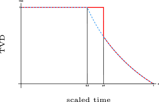 Figure 1
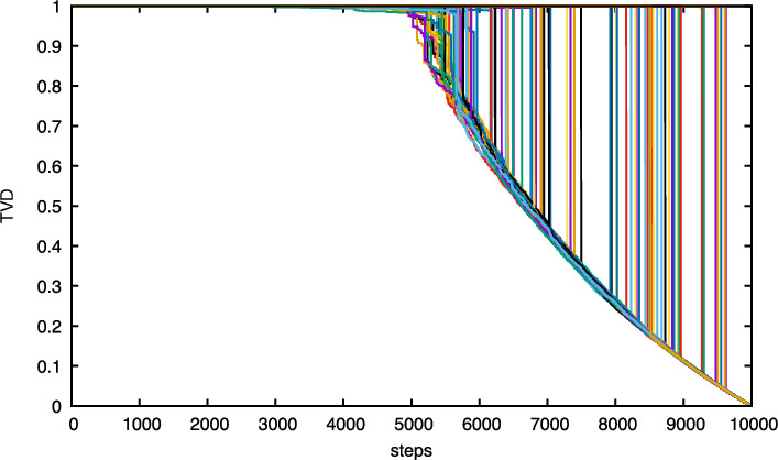 Figure 2
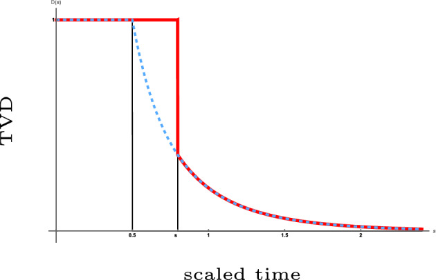 Figure 3
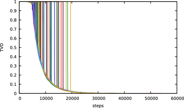 Figure 4
 Figure 5
 Figure 6
 Figure 7
 Figure 8
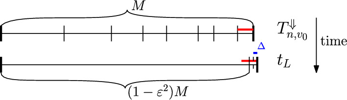 Figure 9
- —http://dx.doi.org/10.13039/501100003246Nederlandse Organisatie voor Wetenschappelijk Onderzoek
Peer Reviews
No public reviews on file for this paper yet. If you reviewed it on a platform where reviews are public (OpenReview, ICLR, NeurIPS, ICML), you can paste yours below so the community can read it here.
Videos
No videos yet. Explain this paper in a talk, walkthrough, or lecture? Add one.
Taxonomy
TopicsStochastic processes and statistical mechanics · Bayesian Methods and Mixture Models · Algorithms and Data Compression
Introduction and main results
Target
The goal of this paper is to identify the mixing profile of a fast random walk on a dynamic random permutation, where fast means that the random walk instantly achieves local equilibrium, i.e., fully mixes on the cycle of the permutation it sits on before the next change in the permutation occurs. The focus is on two types of dynamics for the permutation, both starting from the identity permutation and consisting of successive applications of random transpositions. The first type—called coagulative dynamics—imposes the constraint that transpositions leading to fragmentation of a permutation cycle are ignored. The second type—called coagulative-fragmentative dynamics—does not impose this constraint. A major feature of dynamic random permutations is that they represent a disconnected geometry, which marks a departure from the setting that was considered in earlier work (see Sect. 1.2).
We show that for both dynamics, after scaling time by the length of the permutation and letting this length tend to infinity, the total variation distance between the current distribution and the uniform distribution converges to a limit process that makes a single jump down from the value 1 to a value on a deterministic curve and subsequently follows this curve on its way down to 0. The aforementioned curve is strictly decreasing in time and is related to the size of the largest component in the Erdős–Rényi random graph. The jump down to this curve, which is similar to a one-sided cut-off, occurs after a random time whose law we identify. This type of mixing profile is different from that of previously studied models (see Sect. 1.2). The law of the drop-down time and the function describing the deterministic curve are different for the two types of dynamics. Visual representations of the mixing profiles are given in Figs. 1 and 3, while simulations are shown in Figs. 2 and 4.
The model analysed in this paper is a first step towards understanding the behaviour of simple random walk on a dynamic permutation. This process is, despite its apparent simplicity, hard to analyse in detail, especially when the stepping rate of the random walk is commensurate with the transposition rate of the dynamic permutation. (In Appendix A we show that our model indeed is the limit of the simple random walk model as the step rate tends to infinity.) A key tool in our analysis is Schramm’s coupling [1]. While this coupling was used previously to study the cycle structure of a dynamic permutation at a fixed time, we adapt the arguments in a way that allows us to study the evolution of cycles over a time interval of diverging length. We emphasise that our model is a random walk in a dynamic random environment (i.e., time-inhomogeneous) and therefore has features different from those of a random walk in a static random environment (i.e., time-homogeneous). Moreover, our model can be viewed as a mass-spreading process on a disconnected dynamic geometry, and therefore bridges two perspectives (see e.g. [2], which cites the present paper, and references therein).Fig. 1. The red curve is a typical evolution of the total variation distance for an infinitely fast random walk on a coagulative dynamic permutation. The blue curve is a plot of the deterministic function of the scaled time to which the total variation distance drops at a random time and subsequently sticks toFig. 2Simulations of the evolution of the total variation distance for \documentclass[12pt]{minimal} \usepackage{amsmath} \usepackage{wasysym} \usepackage{amsfonts} \usepackage{amssymb} \usepackage{amsbsy} \usepackage{mathrsfs} \usepackage{upgreek} \setlength{\oddsidemargin}{-69pt} \begin{document}$$10^2$$\end{document} different realisations of a coagulative dynamic permutation of \documentclass[12pt]{minimal} \usepackage{amsmath} \usepackage{wasysym} \usepackage{amsfonts} \usepackage{amssymb} \usepackage{amsbsy} \usepackage{mathrsfs} \usepackage{upgreek} \setlength{\oddsidemargin}{-69pt} \begin{document}$$10^4$$\end{document} elements and an infinitely fast random walk on top. Each simulation run corresponds to a single coloured curveFig. 3The same as Fig. 1 for a coagulative-fragmentative dynamic permutationFig. 4. The same as Fig. 2 for a coagulative-fragmentative permutation
The remainder of this section is organised as follows. Section 1.2 provides background and recalls earlier work. Section 1.3 fixes the setting and introduces relevant definitions and notations. Section 1.4 lists some preliminaries for Erdős–Rényi random graphs that are needed along the way. Section 1.5 introduces a graph process associated with the dynamics that serves as a tool for analysing the dynamics. Section 1.6 contains two main theorems, one for each type of dynamics, describing the evolution of the total variation distance between the current distribution of the random walk and its equilibrium distribution, which is the uniform distribution on \documentclass[12pt]{minimal} \usepackage{amsmath} \usepackage{wasysym} \usepackage{amsfonts} \usepackage{amssymb} \usepackage{amsbsy} \usepackage{mathrsfs} \usepackage{upgreek} \setlength{\oddsidemargin}{-69pt} \begin{document}$$[n]=\{1, \ldots , n\}$$\end{document} . Section 1.7 discusses the importance of the main theorems, places them in their proper context, and provides an outline of the remainder of the paper.
Background and earlier work
While over the past years random walks on static random graphs have received a lot of attention, and the scaling properties of quantities like mixing times, cover times and metastable crossover times have been identified, much less is known about random walks on dynamic random graphs. In the static setting, a two-sided cut-off on scale \documentclass[12pt]{minimal} \usepackage{amsmath} \usepackage{wasysym} \usepackage{amsfonts} \usepackage{amssymb} \usepackage{amsbsy} \usepackage{mathrsfs} \usepackage{upgreek} \setlength{\oddsidemargin}{-69pt} \begin{document}$$\log n$$\end{document} has been established for a general class of undirected sparse graphs with good expansion properties [3–5]. Similar results have been obtained for directed sparse graphs [6, 7] and for graphs with a community structure [8].
In the dynamic setting, predominantly the focus has been on dynamic percolation, Erdős–Rényi random graphs with edges switching on and off randomly, and configuration models with random rewiring of edges. Both directed and undirected graphs have been considered, as well as backtracking and non-backtracking random walks. In [9–11] random walks on dynamic percolation clusters on a d-dimensional discrete torus were considered. Mixing times were identified for several parameter regimes controlling the rate of the random walk and the rate of the random graph dynamics. Similar results were obtained for dynamic percolation on the complete graph [12, 13]. Some further advances were achieved in [14], where general bounds on mixing times, hitting times, cover times and return times were derived for certain classes of dynamic random graphs under appropriate expansion assumptions. Non-backtracking random walks on configuration models that are sparse and with high probability are connected were studied in a series of papers [15–17], which culminated in a general framework for studying mixing times of non-backtracking random walks on dynamic random graphs subject to mild regularity conditions. Mixing of random walks on directed configuration models was treated in [18].
Random permutations generated by random transpositions have attracted plenty of interest as well. An important starting point is [19], where a cut-off in the total variation distance was established after the application of \documentclass[12pt]{minimal} \usepackage{amsmath} \usepackage{wasysym} \usepackage{amsfonts} \usepackage{amssymb} \usepackage{amsbsy} \usepackage{mathrsfs} \usepackage{upgreek} \setlength{\oddsidemargin}{-69pt} \begin{document}$$\frac{1}{2} n\log n + O(n)$$\end{document} random transpositions. The sharp constant in front of the leading-order term was achieved with the help of representation theory for the symmetric group. This paper led to a flurry of follow-up work, of which we mention [1], where the structure of large cycles of an evolving random permutation was studied. Similar results were obtained in [20], including sharp control on the number of observed fragmentations. An important aspect of both [1] and [20] is the representation of an evolving random permutation, starting from the identity permutation, in terms of a random graph process that can be studied by using the theory of random graphs. For the coagulative-fragmentative dynamics considered in the present paper, also called transposition dynamics, this graph process representation yields a graph-growth model that at every step adds an edge drawn uniformly at random. This graph-growth model is closely related to the standard “combinatorial” Erdős–Rényi model, whose study is by now a classical topic in the theory of random graphs (see, for example, [21] or [22]). Yet another important feature of [1] is the introduction of Schramm’s coupling as a tool to study the cycle structure of evolving random permutations. In a follow-up article [23], a modified version of this coupling is used to study the mixing of dynamic permutations endowed with a more general dynamics, of which the transposition dynamics is a special case. We also mention [24], which contains a detailed account of Schramm’s coupling. The works cited above each highlight one particular facet of the random transposition model, but close relatives have been studied extensively under different names: mean-field Tóth model [25], the interchange process on the complete graph (see [24, 26, 27] and references therein), or multi-urn Bernoulli-Laplace diffusion models [28], where our setting corresponds to a particular choice of the model parameters.
The coagulative dynamics considered in the present paper can be recast, in the spirit of [1], as a graph-valued random process that starts with an empty graph on n vertices and describes a forest that progressively merges into a spanning tree on n vertices through the addition of edges that do not create a cycle. The study of this process and its close relatives has a somewhat twisted history. It is similar to the standard additive coalescent (see [29] for an overview), but it is also interesting in its own right (see [30, 31]). Finally, there is a wealth of results on minimal spanning trees and Kruskal’s algorithm, which is another closely related process. In particular, we mention [32], since this work implies some facts that we list in Sect. 2. We derive these facts independently, using different techniques in a different setting.
Setting, definitions and notation
For \documentclass[12pt]{minimal} \usepackage{amsmath} \usepackage{wasysym} \usepackage{amsfonts} \usepackage{amssymb} \usepackage{amsbsy} \usepackage{mathrsfs} \usepackage{upgreek} \setlength{\oddsidemargin}{-69pt} \begin{document}$$n \in {\mathbb {N}}$$\end{document} , let \documentclass[12pt]{minimal} \usepackage{amsmath} \usepackage{wasysym} \usepackage{amsfonts} \usepackage{amssymb} \usepackage{amsbsy} \usepackage{mathrsfs} \usepackage{upgreek} \setlength{\oddsidemargin}{-69pt} \begin{document}$$S_n$$\end{document} denote the set of permutations of [n], i.e., bijections from [n] to itself. Recall that \documentclass[12pt]{minimal} \usepackage{amsmath} \usepackage{wasysym} \usepackage{amsfonts} \usepackage{amssymb} \usepackage{amsbsy} \usepackage{mathrsfs} \usepackage{upgreek} \setlength{\oddsidemargin}{-69pt} \begin{document}$$S_n$$\end{document} endowed with the operation of permutation composition \documentclass[12pt]{minimal} \usepackage{amsmath} \usepackage{wasysym} \usepackage{amsfonts} \usepackage{amssymb} \usepackage{amsbsy} \usepackage{mathrsfs} \usepackage{upgreek} \setlength{\oddsidemargin}{-69pt} \begin{document}$$\circ $$\end{document} forms a group. Write \documentclass[12pt]{minimal} \usepackage{amsmath} \usepackage{wasysym} \usepackage{amsfonts} \usepackage{amssymb} \usepackage{amsbsy} \usepackage{mathrsfs} \usepackage{upgreek} \setlength{\oddsidemargin}{-69pt} \begin{document}$$\gamma _{v}(\pi )$$\end{document} to denote the cycle of the permutation \documentclass[12pt]{minimal} \usepackage{amsmath} \usepackage{wasysym} \usepackage{amsfonts} \usepackage{amssymb} \usepackage{amsbsy} \usepackage{mathrsfs} \usepackage{upgreek} \setlength{\oddsidemargin}{-69pt} \begin{document}$$\pi $$\end{document} that contains the element v.
Definition 1.1
(Dynamic permutation) A sequence of permutations of [n], denoted by \documentclass[12pt]{minimal} \usepackage{amsmath} \usepackage{wasysym} \usepackage{amsfonts} \usepackage{amssymb} \usepackage{amsbsy} \usepackage{mathrsfs} \usepackage{upgreek} \setlength{\oddsidemargin}{-69pt} \begin{document}$$\Pi _n = (\Pi _n(t))_{t=0}^{t^{\textrm{max}}}$$\end{document} with \documentclass[12pt]{minimal} \usepackage{amsmath} \usepackage{wasysym} \usepackage{amsfonts} \usepackage{amssymb} \usepackage{amsbsy} \usepackage{mathrsfs} \usepackage{upgreek} \setlength{\oddsidemargin}{-69pt} \begin{document}$$t^{\textrm{max}} \in {\mathbb {N}}_0 \cup \{\infty \}$$\end{document} , is called a dynamic permutation. \documentclass[12pt]{minimal} \usepackage{amsmath} \usepackage{wasysym} \usepackage{amsfonts} \usepackage{amssymb} \usepackage{amsbsy} \usepackage{mathrsfs} \usepackage{upgreek} \setlength{\oddsidemargin}{-69pt} \begin{document}$$\spadesuit $$\end{document}
Example 1.2
(Transpositions may fragment cycles or coagulate cycles) Pick \documentclass[12pt]{minimal} \usepackage{amsmath} \usepackage{wasysym} \usepackage{amsfonts} \usepackage{amssymb} \usepackage{amsbsy} \usepackage{mathrsfs} \usepackage{upgreek} \setlength{\oddsidemargin}{-69pt} \begin{document}$$n=7$$\end{document} and consider the permutation
\documentclass[12pt]{minimal} \usepackage{amsmath} \usepackage{wasysym} \usepackage{amsfonts} \usepackage{amssymb} \usepackage{amsbsy} \usepackage{mathrsfs} \usepackage{upgreek} \setlength{\oddsidemargin}{-69pt} \begin{document}$$\begin{aligned} \left( \begin{array}{lllllll} 1 & 2 & 3 & 4 & 5 & 6 & 7\\ 2 & 3 & 4 & 5 & 6 & 7 & 1 \end{array}\right) \quad \text {with cycle structure} \quad (1,2,3,4,5,6,7). \end{aligned}$$\end{document}The transposition (1, 5) turns this into the permutation
\documentclass[12pt]{minimal} \usepackage{amsmath} \usepackage{wasysym} \usepackage{amsfonts} \usepackage{amssymb} \usepackage{amsbsy} \usepackage{mathrsfs} \usepackage{upgreek} \setlength{\oddsidemargin}{-69pt} \begin{document}$$\begin{aligned} \left( \begin{array}{lllllll} 1 & 2 & 3 & 4 & 5 & 6 & 7\\ 6 & 3 & 4 & 5 & 2 & 7 & 1 \end{array}\right) \quad \text {with cycle structure} \quad (1,6,7)(2,3,4,5). \end{aligned}$$\end{document}Another application of the same transposition acts in reverse. Note that \documentclass[12pt]{minimal} \usepackage{amsmath} \usepackage{wasysym} \usepackage{amsfonts} \usepackage{amssymb} \usepackage{amsbsy} \usepackage{mathrsfs} \usepackage{upgreek} \setlength{\oddsidemargin}{-69pt} \begin{document}$$S_n$$\end{document} is a non-commutative group for any \documentclass[12pt]{minimal} \usepackage{amsmath} \usepackage{wasysym} \usepackage{amsfonts} \usepackage{amssymb} \usepackage{amsbsy} \usepackage{mathrsfs} \usepackage{upgreek} \setlength{\oddsidemargin}{-69pt} \begin{document}$$n \ge 3$$\end{document} . \documentclass[12pt]{minimal} \usepackage{amsmath} \usepackage{wasysym} \usepackage{amsfonts} \usepackage{amssymb} \usepackage{amsbsy} \usepackage{mathrsfs} \usepackage{upgreek} \setlength{\oddsidemargin}{-69pt} \begin{document}$$\square $$\end{document}
We consider two types of dynamic permutations:
Definition 1.3
(Coagulative dynamic permutation) \documentclass[12pt]{minimal} \usepackage{amsmath} \usepackage{wasysym} \usepackage{amsfonts} \usepackage{amssymb} \usepackage{amsbsy} \usepackage{mathrsfs} \usepackage{upgreek} \setlength{\oddsidemargin}{-69pt} \begin{document}$$\Pi _n = (\Pi _n(t))_{t=0}^{n-1}$$\end{document} is called a coagulative dynamic permutation (CDP) when \documentclass[12pt]{minimal} \usepackage{amsmath} \usepackage{wasysym} \usepackage{amsfonts} \usepackage{amssymb} \usepackage{amsbsy} \usepackage{mathrsfs} \usepackage{upgreek} \setlength{\oddsidemargin}{-69pt} \begin{document}$$\Pi _n(0) = \text {Id}$$\end{document} (i.e., the identity permutation) and
\documentclass[12pt]{minimal} \usepackage{amsmath} \usepackage{wasysym} \usepackage{amsfonts} \usepackage{amssymb} \usepackage{amsbsy} \usepackage{mathrsfs} \usepackage{upgreek} \setlength{\oddsidemargin}{-69pt} \begin{document}$$\begin{aligned} \Pi _n(t) = \Pi _n(t-1) \circ (a,b), \qquad t \in [n-1], \end{aligned}$$\end{document}where, for each \documentclass[12pt]{minimal} \usepackage{amsmath} \usepackage{wasysym} \usepackage{amsfonts} \usepackage{amssymb} \usepackage{amsbsy} \usepackage{mathrsfs} \usepackage{upgreek} \setlength{\oddsidemargin}{-69pt} \begin{document}$$t \in [n-1]$$\end{document} , (a, b) is a random transposition sampled uniformly at random from the set of all transpositions of [n] that satisfy the constraint
\documentclass[12pt]{minimal} \usepackage{amsmath} \usepackage{wasysym} \usepackage{amsfonts} \usepackage{amssymb} \usepackage{amsbsy} \usepackage{mathrsfs} \usepackage{upgreek} \setlength{\oddsidemargin}{-69pt} \begin{document}$$\begin{aligned} \gamma _{a}(\Pi _n(t-1)) \ne \gamma _{b}(\Pi _n(t-1)). \end{aligned}$$\end{document}The latter guarantees that no cycle of \documentclass[12pt]{minimal} \usepackage{amsmath} \usepackage{wasysym} \usepackage{amsfonts} \usepackage{amssymb} \usepackage{amsbsy} \usepackage{mathrsfs} \usepackage{upgreek} \setlength{\oddsidemargin}{-69pt} \begin{document}$$\Pi _n(t-1)$$\end{document} is fragmented by the transposition (a, b). \documentclass[12pt]{minimal} \usepackage{amsmath} \usepackage{wasysym} \usepackage{amsfonts} \usepackage{amssymb} \usepackage{amsbsy} \usepackage{mathrsfs} \usepackage{upgreek} \setlength{\oddsidemargin}{-69pt} \begin{document}$$\square $$\end{document}
Definition 1.4
(Coagulative-fragmentative dynamic permutation) \documentclass[12pt]{minimal} \usepackage{amsmath} \usepackage{wasysym} \usepackage{amsfonts} \usepackage{amssymb} \usepackage{amsbsy} \usepackage{mathrsfs} \usepackage{upgreek} \setlength{\oddsidemargin}{-69pt} \begin{document}$$\Pi _n = (\Pi _n(t))_{t=0}^{\infty }$$\end{document} is called a coagulative-fragmentative dynamic permutation (CFDP) when the same holds as in Definition 1.3, but without the constraint in (2). \documentclass[12pt]{minimal} \usepackage{amsmath} \usepackage{wasysym} \usepackage{amsfonts} \usepackage{amssymb} \usepackage{amsbsy} \usepackage{mathrsfs} \usepackage{upgreek} \setlength{\oddsidemargin}{-69pt} \begin{document}$$\spadesuit $$\end{document}
Remark 1.5
(Time horizon for dynamic permutations and cycle structure) Since CDP starts from the identity permutation, it becomes a permutation with a single cycle after exactly \documentclass[12pt]{minimal} \usepackage{amsmath} \usepackage{wasysym} \usepackage{amsfonts} \usepackage{amssymb} \usepackage{amsbsy} \usepackage{mathrsfs} \usepackage{upgreek} \setlength{\oddsidemargin}{-69pt} \begin{document}$$n-1$$\end{document} steps. Once this happens, there is no permutation that satisfies (2) and the dynamics is trapped. CFDP has no traps and can evolve forever. The structure of cycles is random and the sizes of the large cycles, properly rescaled, converge in distribution to the Poisson-Dirichlet distribution with parameter 1 (see e.g. [1, Theorem 1.1] for a precise statement).
Our aim is to study mixing of fast random walks on both CDP and CFDP. To simplify our analysis, we work with infinite-speed random walks, as defined next:
Definition 1.6
(Infinite-speed random walk on \documentclass[12pt]{minimal} \usepackage{amsmath} \usepackage{wasysym} \usepackage{amsfonts} \usepackage{amssymb} \usepackage{amsbsy} \usepackage{mathrsfs} \usepackage{upgreek} \setlength{\oddsidemargin}{-69pt} \begin{document}$$\Pi _n$$\end{document} ) Fix \documentclass[12pt]{minimal} \usepackage{amsmath} \usepackage{wasysym} \usepackage{amsfonts} \usepackage{amssymb} \usepackage{amsbsy} \usepackage{mathrsfs} \usepackage{upgreek} \setlength{\oddsidemargin}{-69pt} \begin{document}$$\Pi _n$$\end{document} and an element \documentclass[12pt]{minimal} \usepackage{amsmath} \usepackage{wasysym} \usepackage{amsfonts} \usepackage{amssymb} \usepackage{amsbsy} \usepackage{mathrsfs} \usepackage{upgreek} \setlength{\oddsidemargin}{-69pt} \begin{document}$$v_0\in [n]$$\end{document} . Recall that \documentclass[12pt]{minimal} \usepackage{amsmath} \usepackage{wasysym} \usepackage{amsfonts} \usepackage{amssymb} \usepackage{amsbsy} \usepackage{mathrsfs} \usepackage{upgreek} \setlength{\oddsidemargin}{-69pt} \begin{document}$$\gamma _{v}(\Pi _n(t))$$\end{document} is the cycle of \documentclass[12pt]{minimal} \usepackage{amsmath} \usepackage{wasysym} \usepackage{amsfonts} \usepackage{amssymb} \usepackage{amsbsy} \usepackage{mathrsfs} \usepackage{upgreek} \setlength{\oddsidemargin}{-69pt} \begin{document}$$\Pi _n(t)$$\end{document} that contains v. Formally, the infinite-speed random walk (ISRW) starting from \documentclass[12pt]{minimal} \usepackage{amsmath} \usepackage{wasysym} \usepackage{amsfonts} \usepackage{amssymb} \usepackage{amsbsy} \usepackage{mathrsfs} \usepackage{upgreek} \setlength{\oddsidemargin}{-69pt} \begin{document}$$v_0$$\end{document} is a sequence of probability distributions \documentclass[12pt]{minimal} \usepackage{amsmath} \usepackage{wasysym} \usepackage{amsfonts} \usepackage{amssymb} \usepackage{amsbsy} \usepackage{mathrsfs} \usepackage{upgreek} \setlength{\oddsidemargin}{-69pt} \begin{document}$$(\mu ^{n,v_0} (t))_{t\in {\mathbb {N}}_0}$$\end{document} supported on [n], with initial distribution at time \documentclass[12pt]{minimal} \usepackage{amsmath} \usepackage{wasysym} \usepackage{amsfonts} \usepackage{amssymb} \usepackage{amsbsy} \usepackage{mathrsfs} \usepackage{upgreek} \setlength{\oddsidemargin}{-69pt} \begin{document}$$t=0$$\end{document} given by
\documentclass[12pt]{minimal} \usepackage{amsmath} \usepackage{wasysym} \usepackage{amsfonts} \usepackage{amssymb} \usepackage{amsbsy} \usepackage{mathrsfs} \usepackage{upgreek} \setlength{\oddsidemargin}{-69pt} \begin{document}$$\begin{aligned} \mu ^{n,v_0} (0) = \left( \mu ^{n,v_0}_{w}(0)\right) _{w\in [n]}, \end{aligned}$$\end{document}where \documentclass[12pt]{minimal} \usepackage{amsmath} \usepackage{wasysym} \usepackage{amsfonts} \usepackage{amssymb} \usepackage{amsbsy} \usepackage{mathrsfs} \usepackage{upgreek} \setlength{\oddsidemargin}{-69pt} \begin{document}$$\mu ^{n,v_0}_{w}(0)$$\end{document} , the mass at \documentclass[12pt]{minimal} \usepackage{amsmath} \usepackage{wasysym} \usepackage{amsfonts} \usepackage{amssymb} \usepackage{amsbsy} \usepackage{mathrsfs} \usepackage{upgreek} \setlength{\oddsidemargin}{-69pt} \begin{document}$$w \in [n]$$\end{document} at time \documentclass[12pt]{minimal} \usepackage{amsmath} \usepackage{wasysym} \usepackage{amsfonts} \usepackage{amssymb} \usepackage{amsbsy} \usepackage{mathrsfs} \usepackage{upgreek} \setlength{\oddsidemargin}{-69pt} \begin{document}$$t=0$$\end{document} , is given by
\documentclass[12pt]{minimal} \usepackage{amsmath} \usepackage{wasysym} \usepackage{amsfonts} \usepackage{amssymb} \usepackage{amsbsy} \usepackage{mathrsfs} \usepackage{upgreek} \setlength{\oddsidemargin}{-69pt} \begin{document}$$\begin{aligned} \mu ^{n,v_0}_{w}(0) = {\left\{ \begin{array}{ll} \frac{1}{|\gamma _{w}(\Pi _n(0)) |}, & w \in \gamma _{v_0}(\Pi _n(0)),\\ 0, & w \notin \gamma _{v_0}(\Pi _n(0)), \end{array}\right. } \end{aligned}$$\end{document}and with distribution at a later time \documentclass[12pt]{minimal} \usepackage{amsmath} \usepackage{wasysym} \usepackage{amsfonts} \usepackage{amssymb} \usepackage{amsbsy} \usepackage{mathrsfs} \usepackage{upgreek} \setlength{\oddsidemargin}{-69pt} \begin{document}$$t \in {\mathbb {N}}$$\end{document} given by
\documentclass[12pt]{minimal} \usepackage{amsmath} \usepackage{wasysym} \usepackage{amsfonts} \usepackage{amssymb} \usepackage{amsbsy} \usepackage{mathrsfs} \usepackage{upgreek} \setlength{\oddsidemargin}{-69pt} \begin{document}$$\begin{aligned} \mu ^{n,v_0} (t) = \left( \mu ^{n,v_0}_{w}(t)\right) _{w\in [n]}, \end{aligned}$$\end{document}where
\documentclass[12pt]{minimal} \usepackage{amsmath} \usepackage{wasysym} \usepackage{amsfonts} \usepackage{amssymb} \usepackage{amsbsy} \usepackage{mathrsfs} \usepackage{upgreek} \setlength{\oddsidemargin}{-69pt} \begin{document}$$\begin{aligned} \mu ^{n,v_0}_{w}(t) = \frac{1}{|\gamma _{w}(\Pi _n(t))|} \sum _{u \in \gamma _{w}(\Pi _n(t))}\mu ^{n,v_0}_{u}(t-1). \end{aligned}$$\end{document}Informally, ISRW spreads infinitely fast over the cycle in the permutation it resides on. \documentclass[12pt]{minimal} \usepackage{amsmath} \usepackage{wasysym} \usepackage{amsfonts} \usepackage{amssymb} \usepackage{amsbsy} \usepackage{mathrsfs} \usepackage{upgreek} \setlength{\oddsidemargin}{-69pt} \begin{document}$$\spadesuit $$\end{document}
In Appendix A we show that the infinite-speed random walk arises as the limit of a standard random walk whose stepping rate relative to the rate of the permutation dynamics tends to infinity. Note that the evolution of the ISRW distribution is fully determined by the initial position of the random walk and the realisation of the dynamic permutation. See Fig. 5 for an illustration.
Remark 1.7
(ISRW as a mass-spreading process) The reader may prefer to let go of the connection with the random walk and view the ISRW purely as a mass-spreading process. Such a change of perspective would change nothing in our arguments.
Fig. 5. Example of an evolution of an ISRW on top of a CFDP with three elements starting from the identity permutation. The first row shows the transpositions that generate the next permutation. The second row is a graphical representation of the cycles of this permutation. The third row shows the evolution of the ISRW distribution, given that it started from the element 1
Preliminaries for Erdös-Rényi random graphs
The arguments in this paper frequently make use of results on the structure of Erdős–Rényi random graphs. This section provides what is needed to state the main theorems in Sect. 1.6. For overviews on Erdős–Rényi random graphs and their properties we refer to [21, 22, 33–35].
Definition 1.8
(Standard Erdős–Rényi multi-graph process) The standard Erdős–Rényi multi-graph process on n vertices is the discrete-time process \documentclass[12pt]{minimal} \usepackage{amsmath} \usepackage{wasysym} \usepackage{amsfonts} \usepackage{amssymb} \usepackage{amsbsy} \usepackage{mathrsfs} \usepackage{upgreek} \setlength{\oddsidemargin}{-69pt} \begin{document}$$\left( G(n,t) \right) _{t=0}^{t_{\textrm{max}}}$$\end{document} constructed as follows:
- G(n, 0) is the graph with n vertices and no edges.
- At each time \documentclass[12pt]{minimal} \usepackage{amsmath} \usepackage{wasysym} \usepackage{amsfonts} \usepackage{amssymb} \usepackage{amsbsy} \usepackage{mathrsfs} \usepackage{upgreek} \setlength{\oddsidemargin}{-69pt} \begin{document}$$t\in {\mathbb {N}}_0$$\end{document} , pick an edge \documentclass[12pt]{minimal} \usepackage{amsmath} \usepackage{wasysym} \usepackage{amsfonts} \usepackage{amssymb} \usepackage{amsbsy} \usepackage{mathrsfs} \usepackage{upgreek} \setlength{\oddsidemargin}{-69pt} \begin{document}$$e_t$$\end{document} uniformly at random from the \documentclass[12pt]{minimal} \usepackage{amsmath} \usepackage{wasysym} \usepackage{amsfonts} \usepackage{amssymb} \usepackage{amsbsy} \usepackage{mathrsfs} \usepackage{upgreek} \setlength{\oddsidemargin}{-69pt} \begin{document}$$\left( {\begin{array}{c}n\\ 2\end{array}}\right) $$\end{document} possible edges, and let G(n, t) be the graph obtained by adding \documentclass[12pt]{minimal} \usepackage{amsmath} \usepackage{wasysym} \usepackage{amsfonts} \usepackage{amssymb} \usepackage{amsbsy} \usepackage{mathrsfs} \usepackage{upgreek} \setlength{\oddsidemargin}{-69pt} \begin{document}$$e_t$$\end{document} to \documentclass[12pt]{minimal} \usepackage{amsmath} \usepackage{wasysym} \usepackage{amsfonts} \usepackage{amssymb} \usepackage{amsbsy} \usepackage{mathrsfs} \usepackage{upgreek} \setlength{\oddsidemargin}{-69pt} \begin{document}$$G(n, t-1)$$\end{document} . Note that we do not allow for self-loops, but do allow for multiple edges. \documentclass[12pt]{minimal} \usepackage{amsmath} \usepackage{wasysym} \usepackage{amsfonts} \usepackage{amssymb} \usepackage{amsbsy} \usepackage{mathrsfs} \usepackage{upgreek} \setlength{\oddsidemargin}{-69pt} \begin{document}$$\spadesuit $$\end{document}
Remark 1.9
(Versions and asymptotic equivalence) There are versions of the Erdős–Rényi multi-graph process that differ in how edges are deployed and whether or not multiple edges and self-loops are allowed. With respect to monotone properties, notably the expected size of connected components, the “random growth” G(n, t) model described in Definition 1.8 is asymptotically equivalent to the “combinatorial” model G(n, M) with \documentclass[12pt]{minimal} \usepackage{amsmath} \usepackage{wasysym} \usepackage{amsfonts} \usepackage{amssymb} \usepackage{amsbsy} \usepackage{mathrsfs} \usepackage{upgreek} \setlength{\oddsidemargin}{-69pt} \begin{document}$$M = t$$\end{document} edges at times \documentclass[12pt]{minimal} \usepackage{amsmath} \usepackage{wasysym} \usepackage{amsfonts} \usepackage{amssymb} \usepackage{amsbsy} \usepackage{mathrsfs} \usepackage{upgreek} \setlength{\oddsidemargin}{-69pt} \begin{document}$$t=O(n)$$\end{document} , which in turn is asymptotically equivalent to the “bond percolation” model G(n, p) with \documentclass[12pt]{minimal} \usepackage{amsmath} \usepackage{wasysym} \usepackage{amsfonts} \usepackage{amssymb} \usepackage{amsbsy} \usepackage{mathrsfs} \usepackage{upgreek} \setlength{\oddsidemargin}{-69pt} \begin{document}$$\smash {p = M {\left( {\begin{array}{c}n\\ 2\end{array}}\right) }^{-1}}$$\end{document} . For details, see [21, Sections 1.1, 1.3]. Since we work on time scales of order n, we will use this asymptotic equivalence without further notice.
Definition 1.8 allows for some natural modifications, of which one is important for the study of CDP:
Definition 1.10
(Cycle-free Erdős–Rényi graph process) The cycle-free Erdős–Rényi graph process on n vertices is the graph process \documentclass[12pt]{minimal} \usepackage{amsmath} \usepackage{wasysym} \usepackage{amsfonts} \usepackage{amssymb} \usepackage{amsbsy} \usepackage{mathrsfs} \usepackage{upgreek} \setlength{\oddsidemargin}{-69pt} \begin{document}$$\smash {\left( G(n,t)\right) _{t=0}^{t_{\textrm{max}}}}$$\end{document} starting from the empty graph with n vertices, such that at each time t an edge is added that is chosen uniformly at random from the set of edges that do not create a cycle, a multi-edge or a self-loop. Thus, G(n, t) is a forest for all \documentclass[12pt]{minimal} \usepackage{amsmath} \usepackage{wasysym} \usepackage{amsfonts} \usepackage{amssymb} \usepackage{amsbsy} \usepackage{mathrsfs} \usepackage{upgreek} \setlength{\oddsidemargin}{-69pt} \begin{document}$$0 \le t\le t_{\textrm{max}}$$\end{document} . \documentclass[12pt]{minimal} \usepackage{amsmath} \usepackage{wasysym} \usepackage{amsfonts} \usepackage{amssymb} \usepackage{amsbsy} \usepackage{mathrsfs} \usepackage{upgreek} \setlength{\oddsidemargin}{-69pt} \begin{document}$$\spadesuit $$\end{document}
To understand the typical evolution of CDP, we make use of two couplings: one between CDP and cycle-free Erdős–Rényi graph processes, the other between cycle-free Erdős–Rényi graph processes and their standard counterparts. To explain how, we need to introduce three functions that describe key structural properties of these processes:
Definition 1.11
(Functions related to the structure of Erdős–Rényi random graphs)
- Define \documentclass[12pt]{minimal} \usepackage{amsmath} \usepackage{wasysym} \usepackage{amsfonts} \usepackage{amssymb} \usepackage{amsbsy} \usepackage{mathrsfs} \usepackage{upgreek} \setlength{\oddsidemargin}{-69pt} \begin{document}$$\zeta :\, [0, \infty ) \rightarrow [0,1)$$\end{document} as \documentclass[12pt]{minimal} \usepackage{amsmath} \usepackage{wasysym} \usepackage{amsfonts} \usepackage{amssymb} \usepackage{amsbsy} \usepackage{mathrsfs} \usepackage{upgreek} \setlength{\oddsidemargin}{-69pt} \begin{document}$$\zeta (u) = 0$$\end{document} for \documentclass[12pt]{minimal} \usepackage{amsmath} \usepackage{wasysym} \usepackage{amsfonts} \usepackage{amssymb} \usepackage{amsbsy} \usepackage{mathrsfs} \usepackage{upgreek} \setlength{\oddsidemargin}{-69pt} \begin{document}$$u\in [0, \tfrac{1}{2}]$$\end{document} and as the unique positive solution of the equation \documentclass[12pt]{minimal} \usepackage{amsmath} \usepackage{wasysym} \usepackage{amsfonts} \usepackage{amssymb} \usepackage{amsbsy} \usepackage{mathrsfs} \usepackage{upgreek} \setlength{\oddsidemargin}{-69pt} \begin{document}$$1 - \zeta (u) = \text {e}^{-2u\zeta (u)}$$\end{document} for \documentclass[12pt]{minimal} \usepackage{amsmath} \usepackage{wasysym} \usepackage{amsfonts} \usepackage{amssymb} \usepackage{amsbsy} \usepackage{mathrsfs} \usepackage{upgreek} \setlength{\oddsidemargin}{-69pt} \begin{document}$$u \in (\tfrac{1}{2},\infty )$$\end{document} . Note that \documentclass[12pt]{minimal} \usepackage{amsmath} \usepackage{wasysym} \usepackage{amsfonts} \usepackage{amssymb} \usepackage{amsbsy} \usepackage{mathrsfs} \usepackage{upgreek} \setlength{\oddsidemargin}{-69pt} \begin{document}$$\zeta $$\end{document} is non-decreasing and continuous on \documentclass[12pt]{minimal} \usepackage{amsmath} \usepackage{wasysym} \usepackage{amsfonts} \usepackage{amssymb} \usepackage{amsbsy} \usepackage{mathrsfs} \usepackage{upgreek} \setlength{\oddsidemargin}{-69pt} \begin{document}$$[0,\infty )$$\end{document} , and analytic on \documentclass[12pt]{minimal} \usepackage{amsmath} \usepackage{wasysym} \usepackage{amsfonts} \usepackage{amssymb} \usepackage{amsbsy} \usepackage{mathrsfs} \usepackage{upgreek} \setlength{\oddsidemargin}{-69pt} \begin{document}$$(\tfrac{1}{2},\infty )$$\end{document} .
- Define \documentclass[12pt]{minimal} \usepackage{amsmath} \usepackage{wasysym} \usepackage{amsfonts} \usepackage{amssymb} \usepackage{amsbsy} \usepackage{mathrsfs} \usepackage{upgreek} \setlength{\oddsidemargin}{-69pt} \begin{document}$$\phi :\, [0, \infty ) \rightarrow [0,1)$$\end{document} as
Note that \documentclass[12pt]{minimal} \usepackage{amsmath} \usepackage{wasysym} \usepackage{amsfonts} \usepackage{amssymb} \usepackage{amsbsy} \usepackage{mathrsfs} \usepackage{upgreek} \setlength{\oddsidemargin}{-69pt} \begin{document}$$\phi $$\end{document} is strictly increasing and continuous on \documentclass[12pt]{minimal} \usepackage{amsmath} \usepackage{wasysym} \usepackage{amsfonts} \usepackage{amssymb} \usepackage{amsbsy} \usepackage{mathrsfs} \usepackage{upgreek} \setlength{\oddsidemargin}{-69pt} \begin{document}$$[0,\infty )$$\end{document} , and hence has a well-defined inverse \documentclass[12pt]{minimal} \usepackage{amsmath} \usepackage{wasysym} \usepackage{amsfonts} \usepackage{amssymb} \usepackage{amsbsy} \usepackage{mathrsfs} \usepackage{upgreek} \setlength{\oddsidemargin}{-69pt} \begin{document}$$\phi ^{-1}$$\end{document} . Furthermore, the function \documentclass[12pt]{minimal} \usepackage{amsmath} \usepackage{wasysym} \usepackage{amsfonts} \usepackage{amssymb} \usepackage{amsbsy} \usepackage{mathrsfs} \usepackage{upgreek} \setlength{\oddsidemargin}{-69pt} \begin{document}$$\phi $$\end{document} is properly normalised in the sense that \documentclass[12pt]{minimal} \usepackage{amsmath} \usepackage{wasysym} \usepackage{amsfonts} \usepackage{amssymb} \usepackage{amsbsy} \usepackage{mathrsfs} \usepackage{upgreek} \setlength{\oddsidemargin}{-69pt} \begin{document}$$\phi (\infty ) = 1$$\end{document} (see Appendix B). 3. Define \documentclass[12pt]{minimal} \usepackage{amsmath} \usepackage{wasysym} \usepackage{amsfonts} \usepackage{amssymb} \usepackage{amsbsy} \usepackage{mathrsfs} \usepackage{upgreek} \setlength{\oddsidemargin}{-69pt} \begin{document}$$\eta :\, [0,1) \rightarrow [0,1)$$\end{document} as
\documentclass[12pt]{minimal} \usepackage{amsmath} \usepackage{wasysym} \usepackage{amsfonts} \usepackage{amssymb} \usepackage{amsbsy} \usepackage{mathrsfs} \usepackage{upgreek} \setlength{\oddsidemargin}{-69pt} \begin{document}$$\begin{aligned} \eta (w) = \zeta (\phi ^{-1}(w)), \qquad w\in [0,1). \end{aligned}$$\end{document}\documentclass[12pt]{minimal} \usepackage{amsmath} \usepackage{wasysym} \usepackage{amsfonts} \usepackage{amssymb} \usepackage{amsbsy} \usepackage{mathrsfs} \usepackage{upgreek} \setlength{\oddsidemargin}{-69pt} \begin{document}$$\spadesuit $$\end{document}
The functions defined in Definition 1.11 are illustrated in Fig. 6 and have the following interpretation:
- \documentclass[12pt]{minimal} \usepackage{amsmath} \usepackage{wasysym} \usepackage{amsfonts} \usepackage{amssymb} \usepackage{amsbsy} \usepackage{mathrsfs} \usepackage{upgreek} \setlength{\oddsidemargin}{-69pt} \begin{document}$$\zeta (u)$$\end{document} describes the expected size of the largest component of the Erdős–Rényi random graph at time un. For \documentclass[12pt]{minimal} \usepackage{amsmath} \usepackage{wasysym} \usepackage{amsfonts} \usepackage{amssymb} \usepackage{amsbsy} \usepackage{mathrsfs} \usepackage{upgreek} \setlength{\oddsidemargin}{-69pt} \begin{document}$$u \in [0,\infty )$$\end{document} , denote by \documentclass[12pt]{minimal} \usepackage{amsmath} \usepackage{wasysym} \usepackage{amsfonts} \usepackage{amssymb} \usepackage{amsbsy} \usepackage{mathrsfs} \usepackage{upgreek} \setlength{\oddsidemargin}{-69pt} \begin{document}$$|{\mathscr {C}}_{\textrm{max}}^{\textrm{ER}}(n,un)|$$\end{document} the size of the largest connected component in the Erdős–Rényi random graph with n vertices and un edges, and \documentclass[12pt]{minimal} \usepackage{amsmath} \usepackage{wasysym} \usepackage{amsfonts} \usepackage{amssymb} \usepackage{amsbsy} \usepackage{mathrsfs} \usepackage{upgreek} \setlength{\oddsidemargin}{-69pt} \begin{document}$$|{\mathscr {C}}_{\textrm{sec}}^{\textrm{ER}}(n,un)|$$\end{document} the size of the second-largest connected component. Then, by [36], as \documentclass[12pt]{minimal} \usepackage{amsmath} \usepackage{wasysym} \usepackage{amsfonts} \usepackage{amssymb} \usepackage{amsbsy} \usepackage{mathrsfs} \usepackage{upgreek} \setlength{\oddsidemargin}{-69pt} \begin{document}$$n\rightarrow \infty $$\end{document} ,
- The function \documentclass[12pt]{minimal} \usepackage{amsmath} \usepackage{wasysym} \usepackage{amsfonts} \usepackage{amssymb} \usepackage{amsbsy} \usepackage{mathrsfs} \usepackage{upgreek} \setlength{\oddsidemargin}{-69pt} \begin{document}$$\phi $$\end{document} provides the link between the standard and the cycle-free Erdős–Rényi graph process (see Lemmas 2.4–2.5 below).
- \documentclass[12pt]{minimal} \usepackage{amsmath} \usepackage{wasysym} \usepackage{amsfonts} \usepackage{amssymb} \usepackage{amsbsy} \usepackage{mathrsfs} \usepackage{upgreek} \setlength{\oddsidemargin}{-69pt} \begin{document}$$\eta (u)$$\end{document} is the analogue of \documentclass[12pt]{minimal} \usepackage{amsmath} \usepackage{wasysym} \usepackage{amsfonts} \usepackage{amssymb} \usepackage{amsbsy} \usepackage{mathrsfs} \usepackage{upgreek} \setlength{\oddsidemargin}{-69pt} \begin{document}$$\zeta (u)$$\end{document} for the cycle-free Erdős–Rényi graph process at time un, \documentclass[12pt]{minimal} \usepackage{amsmath} \usepackage{wasysym} \usepackage{amsfonts} \usepackage{amssymb} \usepackage{amsbsy} \usepackage{mathrsfs} \usepackage{upgreek} \setlength{\oddsidemargin}{-69pt} \begin{document}$$u\in [0,1]$$\end{document} (see Lemma 2.6 below). Note the change in behaviour of \documentclass[12pt]{minimal} \usepackage{amsmath} \usepackage{wasysym} \usepackage{amsfonts} \usepackage{amssymb} \usepackage{amsbsy} \usepackage{mathrsfs} \usepackage{upgreek} \setlength{\oddsidemargin}{-69pt} \begin{document}$$\zeta ,\phi ,\phi ^{-1},\eta $$\end{document} at \documentclass[12pt]{minimal} \usepackage{amsmath} \usepackage{wasysym} \usepackage{amsfonts} \usepackage{amssymb} \usepackage{amsbsy} \usepackage{mathrsfs} \usepackage{upgreek} \setlength{\oddsidemargin}{-69pt} \begin{document}$$\tfrac{1}{2}$$\end{document} . Note that \documentclass[12pt]{minimal} \usepackage{amsmath} \usepackage{wasysym} \usepackage{amsfonts} \usepackage{amssymb} \usepackage{amsbsy} \usepackage{mathrsfs} \usepackage{upgreek} \setlength{\oddsidemargin}{-69pt} \begin{document}$$\phi ^{-1}$$\end{document} blows up at 1.Fig. 6. Graphs of the functions introduced in Definition 1.11: \documentclass[12pt]{minimal} \usepackage{amsmath} \usepackage{wasysym} \usepackage{amsfonts} \usepackage{amssymb} \usepackage{amsbsy} \usepackage{mathrsfs} \usepackage{upgreek} \setlength{\oddsidemargin}{-69pt} \begin{document}$$\zeta $$\end{document} , \documentclass[12pt]{minimal} \usepackage{amsmath} \usepackage{wasysym} \usepackage{amsfonts} \usepackage{amssymb} \usepackage{amsbsy} \usepackage{mathrsfs} \usepackage{upgreek} \setlength{\oddsidemargin}{-69pt} \begin{document}$$\phi $$\end{document} , respectively, \documentclass[12pt]{minimal} \usepackage{amsmath} \usepackage{wasysym} \usepackage{amsfonts} \usepackage{amssymb} \usepackage{amsbsy} \usepackage{mathrsfs} \usepackage{upgreek} \setlength{\oddsidemargin}{-69pt} \begin{document}$$\phi ^{-1}$$\end{document} (upper curve), \documentclass[12pt]{minimal} \usepackage{amsmath} \usepackage{wasysym} \usepackage{amsfonts} \usepackage{amssymb} \usepackage{amsbsy} \usepackage{mathrsfs} \usepackage{upgreek} \setlength{\oddsidemargin}{-69pt} \begin{document}$$\eta $$\end{document} (lower curve)
Associated graph process
For any dynamic permutation starting from the identity permutation, define the associated graph process as follows:
Definition 1.12
(Graph process associated with \documentclass[12pt]{minimal} \usepackage{amsmath} \usepackage{wasysym} \usepackage{amsfonts} \usepackage{amssymb} \usepackage{amsbsy} \usepackage{mathrsfs} \usepackage{upgreek} \setlength{\oddsidemargin}{-69pt} \begin{document}$$\Pi _n$$\end{document} ) Let \documentclass[12pt]{minimal} \usepackage{amsmath} \usepackage{wasysym} \usepackage{amsfonts} \usepackage{amssymb} \usepackage{amsbsy} \usepackage{mathrsfs} \usepackage{upgreek} \setlength{\oddsidemargin}{-69pt} \begin{document}$$\Pi _n=(\Pi _n(t))_{t=0}^{t_{\textrm{max}}}$$\end{document} with \documentclass[12pt]{minimal} \usepackage{amsmath} \usepackage{wasysym} \usepackage{amsfonts} \usepackage{amssymb} \usepackage{amsbsy} \usepackage{mathrsfs} \usepackage{upgreek} \setlength{\oddsidemargin}{-69pt} \begin{document}$$t_{\textrm{max}} \in {\mathbb {N}}\cup \{ \infty \}$$\end{document} be a dynamic permutation starting from the identity permutation. Construct the associated graph process, denoted by \documentclass[12pt]{minimal} \usepackage{amsmath} \usepackage{wasysym} \usepackage{amsfonts} \usepackage{amssymb} \usepackage{amsbsy} \usepackage{mathrsfs} \usepackage{upgreek} \setlength{\oddsidemargin}{-69pt} \begin{document}$$A_{\Pi _n}$$\end{document} , as follows:
- At time \documentclass[12pt]{minimal} \usepackage{amsmath} \usepackage{wasysym} \usepackage{amsfonts} \usepackage{amssymb} \usepackage{amsbsy} \usepackage{mathrsfs} \usepackage{upgreek} \setlength{\oddsidemargin}{-69pt} \begin{document}$$t=0$$\end{document} , start with the empty graph on the vertex set \documentclass[12pt]{minimal} \usepackage{amsmath} \usepackage{wasysym} \usepackage{amsfonts} \usepackage{amssymb} \usepackage{amsbsy} \usepackage{mathrsfs} \usepackage{upgreek} \setlength{\oddsidemargin}{-69pt} \begin{document}$${\mathcal {V}}= [n]$$\end{document} .
- At times \documentclass[12pt]{minimal} \usepackage{amsmath} \usepackage{wasysym} \usepackage{amsfonts} \usepackage{amssymb} \usepackage{amsbsy} \usepackage{mathrsfs} \usepackage{upgreek} \setlength{\oddsidemargin}{-69pt} \begin{document}$$t\in {\mathbb {N}}$$\end{document} , add the edge \documentclass[12pt]{minimal} \usepackage{amsmath} \usepackage{wasysym} \usepackage{amsfonts} \usepackage{amssymb} \usepackage{amsbsy} \usepackage{mathrsfs} \usepackage{upgreek} \setlength{\oddsidemargin}{-69pt} \begin{document}$$\{a,b\}$$\end{document} , where a, b are such that \documentclass[12pt]{minimal} \usepackage{amsmath} \usepackage{wasysym} \usepackage{amsfonts} \usepackage{amssymb} \usepackage{amsbsy} \usepackage{mathrsfs} \usepackage{upgreek} \setlength{\oddsidemargin}{-69pt} \begin{document}$$\Pi _n(t) = \Pi _n(t-1)\circ (a,b)$$\end{document} . \documentclass[12pt]{minimal} \usepackage{amsmath} \usepackage{wasysym} \usepackage{amsfonts} \usepackage{amssymb} \usepackage{amsbsy} \usepackage{mathrsfs} \usepackage{upgreek} \setlength{\oddsidemargin}{-69pt} \begin{document}$$\spadesuit $$\end{document}
Associated graph processes were used in [1, 20] and follow-up articles to represent the evolution of a general dynamic permutation in terms of a dynamics generated by applying a single transposition at every time step.
A crucial role will be played by the first time when the support of the random walk distribution intersects the largest connected component of the associated graph process:
Definition 1.13
(Largest component of the associated graph process) Denote by \documentclass[12pt]{minimal} \usepackage{amsmath} \usepackage{wasysym} \usepackage{amsfonts} \usepackage{amssymb} \usepackage{amsbsy} \usepackage{mathrsfs} \usepackage{upgreek} \setlength{\oddsidemargin}{-69pt} \begin{document}$${{\mathscr {C}}_{\textrm{max}}({A_{\Pi _n}(t)})}$$\end{document} the set of vertices in the largest connected component in the associated graph process at time t. If such a connected component is not unique, then take all the vertices in all the largest connected components. \documentclass[12pt]{minimal} \usepackage{amsmath} \usepackage{wasysym} \usepackage{amsfonts} \usepackage{amssymb} \usepackage{amsbsy} \usepackage{mathrsfs} \usepackage{upgreek} \setlength{\oddsidemargin}{-69pt} \begin{document}$$\spadesuit $$\end{document}
Remark 1.14
(Possible non-uniqueness of the largest connected component) In situations where we employ Definition 1.13, the largest connected component is unique with high probability. Situations where it is not unique will be of no importance.
Definition 1.15
(Drop-down time) Fix any \documentclass[12pt]{minimal} \usepackage{amsmath} \usepackage{wasysym} \usepackage{amsfonts} \usepackage{amssymb} \usepackage{amsbsy} \usepackage{mathrsfs} \usepackage{upgreek} \setlength{\oddsidemargin}{-69pt} \begin{document}$$\varepsilon _n>0$$\end{document} such that \documentclass[12pt]{minimal} \usepackage{amsmath} \usepackage{wasysym} \usepackage{amsfonts} \usepackage{amssymb} \usepackage{amsbsy} \usepackage{mathrsfs} \usepackage{upgreek} \setlength{\oddsidemargin}{-69pt} \begin{document}$$\varepsilon _n = \omega (n^{-1/3})$$\end{document} and \documentclass[12pt]{minimal} \usepackage{amsmath} \usepackage{wasysym} \usepackage{amsfonts} \usepackage{amssymb} \usepackage{amsbsy} \usepackage{mathrsfs} \usepackage{upgreek} \setlength{\oddsidemargin}{-69pt} \begin{document}$$\varepsilon _n=o(1)$$\end{document} as \documentclass[12pt]{minimal} \usepackage{amsmath} \usepackage{wasysym} \usepackage{amsfonts} \usepackage{amssymb} \usepackage{amsbsy} \usepackage{mathrsfs} \usepackage{upgreek} \setlength{\oddsidemargin}{-69pt} \begin{document}$$n\rightarrow \infty $$\end{document} . The drop-down time is defined as
\documentclass[12pt]{minimal} \usepackage{amsmath} \usepackage{wasysym} \usepackage{amsfonts} \usepackage{amssymb} \usepackage{amsbsy} \usepackage{mathrsfs} \usepackage{upgreek} \setlength{\oddsidemargin}{-69pt} \begin{document}$$\begin{aligned} T^\Downarrow _{n,v_0}= \inf \Big \{t > \tfrac{n}{2}[1+\varepsilon _n]:\, \text {supp}\left( \mu ^{n,v_0} (t)\right) \cap {\mathscr {C}}_{\textrm{max}}(A_{\Pi _n}(t))\ne \emptyset \Big \}. \end{aligned}$$\end{document}\documentclass[12pt]{minimal} \usepackage{amsmath} \usepackage{wasysym} \usepackage{amsfonts} \usepackage{amssymb} \usepackage{amsbsy} \usepackage{mathrsfs} \usepackage{upgreek} \setlength{\oddsidemargin}{-69pt} \begin{document}$$\spadesuit $$\end{document}
Remark 1.16
(Drop-down time and hitting time of the largest permutation cycle) At first sight it might seem unintuitive that the time \documentclass[12pt]{minimal} \usepackage{amsmath} \usepackage{wasysym} \usepackage{amsfonts} \usepackage{amssymb} \usepackage{amsbsy} \usepackage{mathrsfs} \usepackage{upgreek} \setlength{\oddsidemargin}{-69pt} \begin{document}$$T^\Downarrow _{n,v_0}$$\end{document} from Definition 1.15 plays an important role, since it relates to the graph process rather than the permutation process. Given the diffusive nature of ISRW, an arguably more natural candidate would be the first time when the ISRW is supported on the largest permutation cycle. However, the above definition in terms of the associated graph process allows for a unified presentation of our results in different settings, even when the associated graph process at a single time does not provide all the information about the structure of permutation cycles.
For CDP, the drop-down time is the first time when the cycle that contains \documentclass[12pt]{minimal} \usepackage{amsmath} \usepackage{wasysym} \usepackage{amsfonts} \usepackage{amssymb} \usepackage{amsbsy} \usepackage{mathrsfs} \usepackage{upgreek} \setlength{\oddsidemargin}{-69pt} \begin{document}$$v_0$$\end{document} merges with the largest cycle. For CFDP, however, this is not necessarily true because cycles fragment. We therefore define the drop-down time to be the first time when the random walk ‘sees’ the maximal component, see (10). Later, we will see that, in fact, afterwards the mass spreads over \documentclass[12pt]{minimal} \usepackage{amsmath} \usepackage{wasysym} \usepackage{amsfonts} \usepackage{amssymb} \usepackage{amsbsy} \usepackage{mathrsfs} \usepackage{upgreek} \setlength{\oddsidemargin}{-69pt} \begin{document}$${\mathscr {C}}_{\textrm{max}}(A_{\Pi _n}(t))$$\end{document} quickly.
Remark 1.17
(Properties of drop-down time) Clearly, \documentclass[12pt]{minimal} \usepackage{amsmath} \usepackage{wasysym} \usepackage{amsfonts} \usepackage{amssymb} \usepackage{amsbsy} \usepackage{mathrsfs} \usepackage{upgreek} \setlength{\oddsidemargin}{-69pt} \begin{document}$$T^\Downarrow _{n,v_0}$$\end{document} is random. However, if we condition on a particular realisation of \documentclass[12pt]{minimal} \usepackage{amsmath} \usepackage{wasysym} \usepackage{amsfonts} \usepackage{amssymb} \usepackage{amsbsy} \usepackage{mathrsfs} \usepackage{upgreek} \setlength{\oddsidemargin}{-69pt} \begin{document}$$\Pi _n$$\end{document} , then \documentclass[12pt]{minimal} \usepackage{amsmath} \usepackage{wasysym} \usepackage{amsfonts} \usepackage{amssymb} \usepackage{amsbsy} \usepackage{mathrsfs} \usepackage{upgreek} \setlength{\oddsidemargin}{-69pt} \begin{document}$$T^\Downarrow _{n,v_0}$$\end{document} is a deterministic function of the starting point of the random walk. The role of \documentclass[12pt]{minimal} \usepackage{amsmath} \usepackage{wasysym} \usepackage{amsfonts} \usepackage{amssymb} \usepackage{amsbsy} \usepackage{mathrsfs} \usepackage{upgreek} \setlength{\oddsidemargin}{-69pt} \begin{document}$$\varepsilon _n$$\end{document} is to ensure that \documentclass[12pt]{minimal} \usepackage{amsmath} \usepackage{wasysym} \usepackage{amsfonts} \usepackage{amssymb} \usepackage{amsbsy} \usepackage{mathrsfs} \usepackage{upgreek} \setlength{\oddsidemargin}{-69pt} \begin{document}$$T^\Downarrow _{n,v_0}$$\end{document} represents the first time in the supercritical regime when the largest component in the associated Erdős–Rényi graph process coincides with the support of the ISRW, see Sect. 2.1. The choice of \documentclass[12pt]{minimal} \usepackage{amsmath} \usepackage{wasysym} \usepackage{amsfonts} \usepackage{amssymb} \usepackage{amsbsy} \usepackage{mathrsfs} \usepackage{upgreek} \setlength{\oddsidemargin}{-69pt} \begin{document}$$\varepsilon _n$$\end{document} ensures that the drop-down time avoids the critical window, which corresponds to \documentclass[12pt]{minimal} \usepackage{amsmath} \usepackage{wasysym} \usepackage{amsfonts} \usepackage{amssymb} \usepackage{amsbsy} \usepackage{mathrsfs} \usepackage{upgreek} \setlength{\oddsidemargin}{-69pt} \begin{document}$$\smash {\tfrac{n}{2} + O(n^{2/3})}$$\end{document} , yet covers the entire supercritical regime.
Main results
For convenience, we introduce the following shorthand notation:
Definition 1.18
(Total variation distance away from equilibrium) For \documentclass[12pt]{minimal} \usepackage{amsmath} \usepackage{wasysym} \usepackage{amsfonts} \usepackage{amssymb} \usepackage{amsbsy} \usepackage{mathrsfs} \usepackage{upgreek} \setlength{\oddsidemargin}{-69pt} \begin{document}$$v_0\in [n]$$\end{document} , define
\documentclass[12pt]{minimal} \usepackage{amsmath} \usepackage{wasysym} \usepackage{amsfonts} \usepackage{amssymb} \usepackage{amsbsy} \usepackage{mathrsfs} \usepackage{upgreek} \setlength{\oddsidemargin}{-69pt} \begin{document}$$\begin{aligned} {\mathcal {D}}_n^{v_0}(t) = d_{\textrm{TV}} \left( \mu ^{n,v_0} (t) , \textsf {Unif}([n]) \right) , \qquad t \in {\mathbb {N}}_0. \end{aligned}$$\end{document}\documentclass[12pt]{minimal} \usepackage{amsmath} \usepackage{wasysym} \usepackage{amsfonts} \usepackage{amssymb} \usepackage{amsbsy} \usepackage{mathrsfs} \usepackage{upgreek} \setlength{\oddsidemargin}{-69pt} \begin{document}$$\spadesuit $$\end{document}
Our main results are the following two theorems ( \documentclass[12pt]{minimal} \usepackage{amsmath} \usepackage{wasysym} \usepackage{amsfonts} \usepackage{amssymb} \usepackage{amsbsy} \usepackage{mathrsfs} \usepackage{upgreek} \setlength{\oddsidemargin}{-69pt} \begin{document}$${\mathop {\rightarrow }\limits ^{d}}$$\end{document} denotes convergence in distribution):
Theorem 1.19
(Mixing profile for ISRW on CDP)
- For any fixed \documentclass[12pt]{minimal} \usepackage{amsmath} \usepackage{wasysym} \usepackage{amsfonts} \usepackage{amssymb} \usepackage{amsbsy} \usepackage{mathrsfs} \usepackage{upgreek} \setlength{\oddsidemargin}{-69pt} \begin{document}$$v_0\in [n]$$\end{document} ,
where \documentclass[12pt]{minimal} \usepackage{amsmath} \usepackage{wasysym} \usepackage{amsfonts} \usepackage{amssymb} \usepackage{amsbsy} \usepackage{mathrsfs} \usepackage{upgreek} \setlength{\oddsidemargin}{-69pt} \begin{document}$$s^\Downarrow $$\end{document} is the [0, 1]-valued random variable with distribution (recall (8))
\documentclass[12pt]{minimal} \usepackage{amsmath} \usepackage{wasysym} \usepackage{amsfonts} \usepackage{amssymb} \usepackage{amsbsy} \usepackage{mathrsfs} \usepackage{upgreek} \setlength{\oddsidemargin}{-69pt} \begin{document}$$\begin{aligned} {\mathbb {P}}(s^\Downarrow \le s) = \eta (s),\qquad s\in [0,1]. \end{aligned}$$\end{document}- For any fixed \documentclass[12pt]{minimal} \usepackage{amsmath} \usepackage{wasysym} \usepackage{amsfonts} \usepackage{amssymb} \usepackage{amsbsy} \usepackage{mathrsfs} \usepackage{upgreek} \setlength{\oddsidemargin}{-69pt} \begin{document}$$v_0\in [n]$$\end{document} ,
Theorem 1.20
(Mixing profile for ISRW on CFDP)
- For any fixed \documentclass[12pt]{minimal} \usepackage{amsmath} \usepackage{wasysym} \usepackage{amsfonts} \usepackage{amssymb} \usepackage{amsbsy} \usepackage{mathrsfs} \usepackage{upgreek} \setlength{\oddsidemargin}{-69pt} \begin{document}$$v_0\in [n]$$\end{document} ,
where \documentclass[12pt]{minimal} \usepackage{amsmath} \usepackage{wasysym} \usepackage{amsfonts} \usepackage{amssymb} \usepackage{amsbsy} \usepackage{mathrsfs} \usepackage{upgreek} \setlength{\oddsidemargin}{-69pt} \begin{document}$$u^\Downarrow $$\end{document} is the non-negative random variable with distribution (recall Definition 1.11(1))
\documentclass[12pt]{minimal} \usepackage{amsmath} \usepackage{wasysym} \usepackage{amsfonts} \usepackage{amssymb} \usepackage{amsbsy} \usepackage{mathrsfs} \usepackage{upgreek} \setlength{\oddsidemargin}{-69pt} \begin{document}$$\begin{aligned} {\mathbb {P}}(u^\Downarrow \le u) = \zeta (u), \qquad u\in [0,\infty ). \end{aligned}$$\end{document}- For any fixed \documentclass[12pt]{minimal} \usepackage{amsmath} \usepackage{wasysym} \usepackage{amsfonts} \usepackage{amssymb} \usepackage{amsbsy} \usepackage{mathrsfs} \usepackage{upgreek} \setlength{\oddsidemargin}{-69pt} \begin{document}$$v_0\in [n]$$\end{document} ,
The proofs of these theorems are given in Sects. 2 and 3, respectively. Since the a.s. unique discontinuity in the limiting process arises from an “accumulation” of many small discontinuities observed in the processes for finite n, the Skorokhod \documentclass[12pt]{minimal} \usepackage{amsmath} \usepackage{wasysym} \usepackage{amsfonts} \usepackage{amssymb} \usepackage{amsbsy} \usepackage{mathrsfs} \usepackage{upgreek} \setlength{\oddsidemargin}{-69pt} \begin{document}$$M_1$$\end{document} -topology is the natural setting for our process convergence. We refer the reader to [37, Section 11.5] for an introduction to the Skorokhod \documentclass[12pt]{minimal} \usepackage{amsmath} \usepackage{wasysym} \usepackage{amsfonts} \usepackage{amssymb} \usepackage{amsbsy} \usepackage{mathrsfs} \usepackage{upgreek} \setlength{\oddsidemargin}{-69pt} \begin{document}$$M_1$$\end{document} -topology, as well as the other topologies introduced by Skorokhod in [38]. Also, due to the mismatch between discontinuities in the limiting process and the pre-limit processes, we expect that convergence in the usual Skorokhod \documentclass[12pt]{minimal} \usepackage{amsmath} \usepackage{wasysym} \usepackage{amsfonts} \usepackage{amssymb} \usepackage{amsbsy} \usepackage{mathrsfs} \usepackage{upgreek} \setlength{\oddsidemargin}{-69pt} \begin{document}$$J_1$$\end{document} -topology does not hold. Our results apply to any deterministic \documentclass[12pt]{minimal} \usepackage{amsmath} \usepackage{wasysym} \usepackage{amsfonts} \usepackage{amssymb} \usepackage{amsbsy} \usepackage{mathrsfs} \usepackage{upgreek} \setlength{\oddsidemargin}{-69pt} \begin{document}$$v_0\in [n]$$\end{document} , since, by exchangeability w.r.t. the initial condition, the law of the process does not depend on \documentclass[12pt]{minimal} \usepackage{amsmath} \usepackage{wasysym} \usepackage{amsfonts} \usepackage{amssymb} \usepackage{amsbsy} \usepackage{mathrsfs} \usepackage{upgreek} \setlength{\oddsidemargin}{-69pt} \begin{document}$$v_0$$\end{document} .
Discussion
1. Despite the similarity of Theorems 1.19–1.20, the latter is far more delicate. For CDP, mixing is simply induced by the ISRW entering the ever-growing largest cycle. For CFDP, the presence of fragmentations breaks the direct link between the dynamic permutation and its associated graph process: a single connected component may carry more than one permutation cycle. Specifically, the largest component of the associated graph process carries a large number of permutation cycles and, at the drop-down time, the distribution of the ISRW is supported on only one of them. It is not a priori clear how many steps the dynamics needs to spread out the ISRW distribution over all the elements that lie on the largest component of the associated graph process. Therefore, a major hurdle in the proof of Theorem 1.20 is to show that such local mixing happens on time scale o(n). We actually show a stronger statement, namely, that local mixing occurs on an arbitrarily small but diverging time scale (see Sect. 3.3 for details). The core of the proof is to show that on the largest component over time there is a diverging count of appearances of permutation cycles that span almost the entire largest component of the associated graph process.
2. Theorems 1.19–1.20 extend our earlier results for the total variation distance of a (non-backtracking) random walk on a configuration model subject to random rewirings [17]. There we assumed that all the degrees are at least three, which corresponds to a supercritical configuration model that with high probability is connected (see [35, Chapter 4]). Our model with evolving permutation cycles is closely related to the setting where all the degrees are two, which in turn corresponds to a special kind of configuration model that with high probability is disconnected (see Fig. 7). In this setting, even small perturbations of the degree sequence can lead to significantly different behaviour (see [39] for details). In Appendix E we comment further on the connection between permutations and degree-two graphs. More concretely, we show that in the setting of dynamic degree-two graphs with rewiring, we obtain an ISRW-mixing profile analogous to the one described in Theorem 1.20 (see Theorem E.3). We stress that in the present work the starting configuration is fixed to be the identity permutation, which would correspond to a graph with only self-loops, whereas in our previous work the starting configuration was sampled from the configuration model.Fig. 7. Dynamic permutations are similar to rewirings in the configuration model, where all degrees are two. Recall Example 1.2. Consider the permutation \documentclass[12pt]{minimal} \usepackage{amsmath} \usepackage{wasysym} \usepackage{amsfonts} \usepackage{amssymb} \usepackage{amsbsy} \usepackage{mathrsfs} \usepackage{upgreek} \setlength{\oddsidemargin}{-69pt} \begin{document}$$\Pi (0) = (1,2,3,4,5,6,7)$$\end{document} , which consists of a single cycle and corresponds to a degree-two graph that has a single connected component. Apply the transposition (1, 5) to get a new permutation \documentclass[12pt]{minimal} \usepackage{amsmath} \usepackage{wasysym} \usepackage{amsfonts} \usepackage{amssymb} \usepackage{amsbsy} \usepackage{mathrsfs} \usepackage{upgreek} \setlength{\oddsidemargin}{-69pt} \begin{document}$$\Pi (1) = \Pi (0) \circ (1,5) = (1,6,7) (2,3,4,5)$$\end{document} , which consists of two cycles and corresponds to a degree-two graph that has two connected components, obtained by sampling the edges \documentclass[12pt]{minimal} \usepackage{amsmath} \usepackage{wasysym} \usepackage{amsfonts} \usepackage{amssymb} \usepackage{amsbsy} \usepackage{mathrsfs} \usepackage{upgreek} \setlength{\oddsidemargin}{-69pt} \begin{document}$$(1,\Pi (0)(1)) = (1,2)$$\end{document} and \documentclass[12pt]{minimal} \usepackage{amsmath} \usepackage{wasysym} \usepackage{amsfonts} \usepackage{amssymb} \usepackage{amsbsy} \usepackage{mathrsfs} \usepackage{upgreek} \setlength{\oddsidemargin}{-69pt} \begin{document}$$(5,\Pi (0)(5)) = (5,6)$$\end{document} and rewiring them
3. The mixing profile in Theorems 1.19–1.20 is novel: the total variation distance makes a single jump down from the value 1 to a value on a deterministic curve and subsequently follows this curve on its way down to 0. This jump, which is similar to a one-sided cut-off, occurs after a random time. The law of the drop-down time and the function describing the deterministic curve depend on the choice of dynamics.
4. The pathwise statements in part (2) of Theorems 1.19–1.20 imply the following pointwise statements ( \documentclass[12pt]{minimal} \usepackage{amsmath} \usepackage{wasysym} \usepackage{amsfonts} \usepackage{amssymb} \usepackage{amsbsy} \usepackage{mathrsfs} \usepackage{upgreek} \setlength{\oddsidemargin}{-69pt} \begin{document}$$\sim $$\end{document} denotes equality in distribution):
\documentclass[12pt]{minimal} \usepackage{amsmath} \usepackage{wasysym} \usepackage{amsfonts} \usepackage{amssymb} \usepackage{amsbsy} \usepackage{mathrsfs} \usepackage{upgreek} \setlength{\oddsidemargin}{-69pt} \begin{document}$$\begin{aligned} \begin{array}{lll} & {\mathcal {D}}_n^{v_0}(sn) {\mathop {\rightarrow }\limits ^{d}}1 - \eta (s)Y(s), \quad s \in [0,1], & \text { with } Y(s)\sim \textsf {Bernoulli}(\eta (s)),\\ & {\mathcal {D}}_n^{v_0}(sn) {\mathop {\rightarrow }\limits ^{d}}1 - \zeta (s){{\bar{Y}}}(s), \quad s \in [0,\infty ), & \text { with } {{\bar{Y}}}(s)\sim \textsf {Bernoulli}(\zeta (s)). \end{array} \end{aligned}$$\end{document}Through the function \documentclass[12pt]{minimal} \usepackage{amsmath} \usepackage{wasysym} \usepackage{amsfonts} \usepackage{amssymb} \usepackage{amsbsy} \usepackage{mathrsfs} \usepackage{upgreek} \setlength{\oddsidemargin}{-69pt} \begin{document}$$\phi $$\end{document} plotted in Fig. 6, we can view the two mixing profiles as a continuous deformation of one another. Slower mixing for CFDP is intuitive: fragmentation slows down the mixing, while coagulation enhances it.
5. Note the similarities between the mixing profiles described by Theorems 1.19–1.20. Both feature a single macroscopic jump at a random time to a deterministic curve that depends on the choice of the dynamics. We expect this type of behaviour to occur for any permutation dynamics whose associated graph process exhibits scaling behaviour similar to that of the Erdős–Rényi graph process. A class of graph processes that fits this criterion is the class of Achlioptas processes with bounded-size rules (see [40] or [41]).
6. We can formulate conjectures about finite-speed random walks as well. Settings where the random walk rate dominates are easy to handle. If the random walk is fast enough to ensure local mixing (e.g. \documentclass[12pt]{minimal} \usepackage{amsmath} \usepackage{wasysym} \usepackage{amsfonts} \usepackage{amssymb} \usepackage{amsbsy} \usepackage{mathrsfs} \usepackage{upgreek} \setlength{\oddsidemargin}{-69pt} \begin{document}$$\gg n^2$$\end{document} steps of the random walk occur for every step of the random permutation), then our theorems should remain the same with negligible error terms. In this regime, the mixing is fully driven by the underlying geometry. However, once these rates are commensurate, we would have to deal with random walk distributions that are partially mixed over cycles, meaning that the distribution of the random walk would not be uniform over its supporting cycle before this cycle is affected by the permutation dynamics.
7. Dynamic permutations are a natural model for discrete dynamic random environments, which typically are disconnected but nonetheless allow for interaction between their constitutive elements. We believe this setting to be interesting for other stochastic processes on random graphs as well, such as the voter model or the contact process.
Organisation of the paper.
Section 2 starts by establishing a link between CDP and cycle-free Erdős–Rényi random graphs. A coupling construction is employed to describe the cyclic structure of a typical CDP. These results are used to prove Theorem 1.19. Section 3 deals with CFDP, where the main problem is that the associated graph process provides weaker control over permutation cycles than for CDP. After this discrepancy is settled, we employ arguments analogous to those in Sect. 2 to prove Theorem 1.20.
Appendices A–B contain supplementary material that is not needed in Sects. 2–3. Namely, Appendix A shows that the ISRW arises as a fast-speed limit of the standard random walk. Appendix B proves that the laws of the jump-down times in Theorems 1.19–1.20 are properly normalised. Appendix C contains the key coupling that is used to study the cycle structure of CFDP, which is technical and of interest in itself. This coupling is needed in Sect. 3. Appendix D contains a technical computation that is needed in Sect. 3 as well. Finally, Appendix E elucidates the connection between random permutations and graphs with all the degrees equal to two and extends Theorem 1.20 to the setting of dynamic degree-two graphs.
Coagulative dynamic permutations
In this section, we establish a link between dynamic permutations and evolving graphs. To do so, we couple a CDP with a cycle-free Erdős–Rényi graph process (Sect. 2.1), and couple the latter with the standard Erdős–Rényi graph process (Sect. 2.2) by making use of well-known results on the structure of connected components of Erdős–Rényi random graphs (recall Sect. 1.4). We use the couplings to prove Theorem 1.19 (Sect. 2.3).
Representation via associated graph process
Note that for the dynamics generated by transpositions sampled uniformly at random from the set of all transpositions of n elements, the associated graph process is equal in distribution to the Erdős–Rényi process defined in Definition 1.8. In the setting of coagulative dynamic transpositions, this leads us to the following observation:
Lemma 2.1
(Representation of CDP as cycle-free graph process) If \documentclass[12pt]{minimal} \usepackage{amsmath} \usepackage{wasysym} \usepackage{amsfonts} \usepackage{amssymb} \usepackage{amsbsy} \usepackage{mathrsfs} \usepackage{upgreek} \setlength{\oddsidemargin}{-69pt} \begin{document}$$\Pi _n$$\end{document} is a CDP, then its associated graph process \documentclass[12pt]{minimal} \usepackage{amsmath} \usepackage{wasysym} \usepackage{amsfonts} \usepackage{amssymb} \usepackage{amsbsy} \usepackage{mathrsfs} \usepackage{upgreek} \setlength{\oddsidemargin}{-69pt} \begin{document}$$A_{\Pi _n}$$\end{document} is the cycle-free Erdős–Rényi graph process defined in Definition 1.10.
Proof
Recall that the change between two successive permutations in a CDP is generated by applying a single transposition. Furthermore, note that the only transpositions causing a split of a permutation cycle are the ones that transpose two elements from the same cycle. Recall Definition 1.12, and note that if \documentclass[12pt]{minimal} \usepackage{amsmath} \usepackage{wasysym} \usepackage{amsfonts} \usepackage{amssymb} \usepackage{amsbsy} \usepackage{mathrsfs} \usepackage{upgreek} \setlength{\oddsidemargin}{-69pt} \begin{document}$$A_{\Pi _n}(t)$$\end{document} is a forest, then its connected components correspond to cycles of \documentclass[12pt]{minimal} \usepackage{amsmath} \usepackage{wasysym} \usepackage{amsfonts} \usepackage{amssymb} \usepackage{amsbsy} \usepackage{mathrsfs} \usepackage{upgreek} \setlength{\oddsidemargin}{-69pt} \begin{document}$$\Pi _n(t)$$\end{document} . Furthermore, observe that cycle-splitting transpositions correspond to edges that join two vertices from the same connected component. Thus, if \documentclass[12pt]{minimal} \usepackage{amsmath} \usepackage{wasysym} \usepackage{amsfonts} \usepackage{amssymb} \usepackage{amsbsy} \usepackage{mathrsfs} \usepackage{upgreek} \setlength{\oddsidemargin}{-69pt} \begin{document}$$A_{\Pi _n}(t)$$\end{document} is a forest, then any transposition causing a fragmentation of a permutation cycle corresponds to an edge that creates a cycle in the associated graph process.
Observe that the associated graph process always starts as a forest. Since fragmentations of permutation cycles are not allowed, there can be no edges that lead to graph cycles in the associated graph process. Since the associated graph process for a dynamic permutation with no constraints is the Erdős–Rényi graph process, the associated graph process for a CDP is the Erdős–Rényi graph process constrained to be a forest (see Definition 1.10). \documentclass[12pt]{minimal} \usepackage{amsmath} \usepackage{wasysym} \usepackage{amsfonts} \usepackage{amssymb} \usepackage{amsbsy} \usepackage{mathrsfs} \usepackage{upgreek} \setlength{\oddsidemargin}{-69pt} \begin{document}$$\square $$\end{document}
Connected components of the cycle-free Erdős–Rényi graph process
\documentclass[12pt]{minimal} \usepackage{amsmath} \usepackage{wasysym} \usepackage{amsfonts} \usepackage{amssymb} \usepackage{amsbsy} \usepackage{mathrsfs} \usepackage{upgreek} \setlength{\oddsidemargin}{-69pt} \begin{document}$$\bullet $$\end{document} Coupling of Erdős–Rényi graph processes.
We construct a coupling of the standard and the cycle-free Erdős–Rényi graph process that allows us to study the structure of the connected components of the cycle-free process.
Definition 2.2
(Coupling between cycle-free and standard Erdős–Rényi graph process) Let \documentclass[12pt]{minimal} \usepackage{amsmath} \usepackage{wasysym} \usepackage{amsfonts} \usepackage{amssymb} \usepackage{amsbsy} \usepackage{mathrsfs} \usepackage{upgreek} \setlength{\oddsidemargin}{-69pt} \begin{document}$$G_n = (G_n(t))_{t\in {\mathbb {N}}_0}$$\end{document} be the Erdős–Rényi graph process on [n] defined in Definition 1.8, and denote the edge set of \documentclass[12pt]{minimal} \usepackage{amsmath} \usepackage{wasysym} \usepackage{amsfonts} \usepackage{amssymb} \usepackage{amsbsy} \usepackage{mathrsfs} \usepackage{upgreek} \setlength{\oddsidemargin}{-69pt} \begin{document}$$G_n(t)$$\end{document} by \documentclass[12pt]{minimal} \usepackage{amsmath} \usepackage{wasysym} \usepackage{amsfonts} \usepackage{amssymb} \usepackage{amsbsy} \usepackage{mathrsfs} \usepackage{upgreek} \setlength{\oddsidemargin}{-69pt} \begin{document}$${\mathcal {E}}_{G_n(t)}$$\end{document} . Based on \documentclass[12pt]{minimal} \usepackage{amsmath} \usepackage{wasysym} \usepackage{amsfonts} \usepackage{amssymb} \usepackage{amsbsy} \usepackage{mathrsfs} \usepackage{upgreek} \setlength{\oddsidemargin}{-69pt} \begin{document}$$G_n$$\end{document} , construct a graph-valued process \documentclass[12pt]{minimal} \usepackage{amsmath} \usepackage{wasysym} \usepackage{amsfonts} \usepackage{amssymb} \usepackage{amsbsy} \usepackage{mathrsfs} \usepackage{upgreek} \setlength{\oddsidemargin}{-69pt} \begin{document}$$F_n = (F_n(t))_{t\in {\mathbb {N}}_0}$$\end{document} as follows:
- \documentclass[12pt]{minimal} \usepackage{amsmath} \usepackage{wasysym} \usepackage{amsfonts} \usepackage{amssymb} \usepackage{amsbsy} \usepackage{mathrsfs} \usepackage{upgreek} \setlength{\oddsidemargin}{-69pt} \begin{document}$$F_n(0)$$\end{document} is the empty graph with vertex set [n].
- At times \documentclass[12pt]{minimal} \usepackage{amsmath} \usepackage{wasysym} \usepackage{amsfonts} \usepackage{amssymb} \usepackage{amsbsy} \usepackage{mathrsfs} \usepackage{upgreek} \setlength{\oddsidemargin}{-69pt} \begin{document}$$t\in {\mathbb {N}}$$\end{document} , define \documentclass[12pt]{minimal} \usepackage{amsmath} \usepackage{wasysym} \usepackage{amsfonts} \usepackage{amssymb} \usepackage{amsbsy} \usepackage{mathrsfs} \usepackage{upgreek} \setlength{\oddsidemargin}{-69pt} \begin{document}$$e^\star (t) = {\mathcal {E}}_{G_n(t)} {\setminus } {\mathcal {E}}_{G_n(t-1)}$$\end{document} , which is the edge added at time t to \documentclass[12pt]{minimal} \usepackage{amsmath} \usepackage{wasysym} \usepackage{amsfonts} \usepackage{amssymb} \usepackage{amsbsy} \usepackage{mathrsfs} \usepackage{upgreek} \setlength{\oddsidemargin}{-69pt} \begin{document}$$G_n(t)$$\end{document} .
- Construct the candidate graph at time t, defined as \documentclass[12pt]{minimal} \usepackage{amsmath} \usepackage{wasysym} \usepackage{amsfonts} \usepackage{amssymb} \usepackage{amsbsy} \usepackage{mathrsfs} \usepackage{upgreek} \setlength{\oddsidemargin}{-69pt} \begin{document}$$F_{n}^{\star }(t) = ({\mathcal {V}}, {\mathcal {E}}_{F_n(t-1)} \cup \{e^\star (t)\})$$\end{document} .
- If \documentclass[12pt]{minimal} \usepackage{amsmath} \usepackage{wasysym} \usepackage{amsfonts} \usepackage{amssymb} \usepackage{amsbsy} \usepackage{mathrsfs} \usepackage{upgreek} \setlength{\oddsidemargin}{-69pt} \begin{document}$$F_{n}^{\star }(t)$$\end{document} is a forest, then set \documentclass[12pt]{minimal} \usepackage{amsmath} \usepackage{wasysym} \usepackage{amsfonts} \usepackage{amssymb} \usepackage{amsbsy} \usepackage{mathrsfs} \usepackage{upgreek} \setlength{\oddsidemargin}{-69pt} \begin{document}$$F_n(t) = F_{n}^{\star }(t)$$\end{document} .
- Otherwise, set \documentclass[12pt]{minimal} \usepackage{amsmath} \usepackage{wasysym} \usepackage{amsfonts} \usepackage{amssymb} \usepackage{amsbsy} \usepackage{mathrsfs} \usepackage{upgreek} \setlength{\oddsidemargin}{-69pt} \begin{document}$$F_{n}(t) = F_{n}(t-1)$$\end{document} . Define the effective time \documentclass[12pt]{minimal} \usepackage{amsmath} \usepackage{wasysym} \usepackage{amsfonts} \usepackage{amssymb} \usepackage{amsbsy} \usepackage{mathrsfs} \usepackage{upgreek} \setlength{\oddsidemargin}{-69pt} \begin{document}$$\tau _n(t)$$\end{document} of the coupled process \documentclass[12pt]{minimal} \usepackage{amsmath} \usepackage{wasysym} \usepackage{amsfonts} \usepackage{amssymb} \usepackage{amsbsy} \usepackage{mathrsfs} \usepackage{upgreek} \setlength{\oddsidemargin}{-69pt} \begin{document}$$(F_n(t))_{t\in {\mathbb {N}}_0}$$\end{document} by setting \documentclass[12pt]{minimal} \usepackage{amsmath} \usepackage{wasysym} \usepackage{amsfonts} \usepackage{amssymb} \usepackage{amsbsy} \usepackage{mathrsfs} \usepackage{upgreek} \setlength{\oddsidemargin}{-69pt} \begin{document}$$\tau _n(0) = 0$$\end{document} and, recursively for \documentclass[12pt]{minimal} \usepackage{amsmath} \usepackage{wasysym} \usepackage{amsfonts} \usepackage{amssymb} \usepackage{amsbsy} \usepackage{mathrsfs} \usepackage{upgreek} \setlength{\oddsidemargin}{-69pt} \begin{document}$$t \in {\mathbb {N}}$$\end{document} ,
Note that \documentclass[12pt]{minimal} \usepackage{amsmath} \usepackage{wasysym} \usepackage{amsfonts} \usepackage{amssymb} \usepackage{amsbsy} \usepackage{mathrsfs} \usepackage{upgreek} \setlength{\oddsidemargin}{-69pt} \begin{document}$$\tau _n(t)$$\end{document} is a random variable because it is a function of a random graph process. We suppress the dependence of \documentclass[12pt]{minimal} \usepackage{amsmath} \usepackage{wasysym} \usepackage{amsfonts} \usepackage{amssymb} \usepackage{amsbsy} \usepackage{mathrsfs} \usepackage{upgreek} \setlength{\oddsidemargin}{-69pt} \begin{document}$$\tau _n(t)$$\end{document} on \documentclass[12pt]{minimal} \usepackage{amsmath} \usepackage{wasysym} \usepackage{amsfonts} \usepackage{amssymb} \usepackage{amsbsy} \usepackage{mathrsfs} \usepackage{upgreek} \setlength{\oddsidemargin}{-69pt} \begin{document}$$F_n$$\end{document} , since we will never work with more than one set of coupled processes at a time. \documentclass[12pt]{minimal} \usepackage{amsmath} \usepackage{wasysym} \usepackage{amsfonts} \usepackage{amssymb} \usepackage{amsbsy} \usepackage{mathrsfs} \usepackage{upgreek} \setlength{\oddsidemargin}{-69pt} \begin{document}$$\spadesuit $$\end{document}
Remark 2.3
(Relation between \documentclass[12pt]{minimal} \usepackage{amsmath} \usepackage{wasysym} \usepackage{amsfonts} \usepackage{amssymb} \usepackage{amsbsy} \usepackage{mathrsfs} \usepackage{upgreek} \setlength{\oddsidemargin}{-69pt} \begin{document}$$F_n$$\end{document} and \documentclass[12pt]{minimal} \usepackage{amsmath} \usepackage{wasysym} \usepackage{amsfonts} \usepackage{amssymb} \usepackage{amsbsy} \usepackage{mathrsfs} \usepackage{upgreek} \setlength{\oddsidemargin}{-69pt} \begin{document}$$A_{\Pi _n}$$\end{document} ) By the definition of the coupling, if there are edge-rejections at times \documentclass[12pt]{minimal} \usepackage{amsmath} \usepackage{wasysym} \usepackage{amsfonts} \usepackage{amssymb} \usepackage{amsbsy} \usepackage{mathrsfs} \usepackage{upgreek} \setlength{\oddsidemargin}{-69pt} \begin{document}$$\{t, t+1, t+2, \ldots , t+k\}$$\end{document} , then a string of \documentclass[12pt]{minimal} \usepackage{amsmath} \usepackage{wasysym} \usepackage{amsfonts} \usepackage{amssymb} \usepackage{amsbsy} \usepackage{mathrsfs} \usepackage{upgreek} \setlength{\oddsidemargin}{-69pt} \begin{document}$$k+1$$\end{document} copies of the same graph is observed in \documentclass[12pt]{minimal} \usepackage{amsmath} \usepackage{wasysym} \usepackage{amsfonts} \usepackage{amssymb} \usepackage{amsbsy} \usepackage{mathrsfs} \usepackage{upgreek} \setlength{\oddsidemargin}{-69pt} \begin{document}$$F_n$$\end{document} , i.e., \documentclass[12pt]{minimal} \usepackage{amsmath} \usepackage{wasysym} \usepackage{amsfonts} \usepackage{amssymb} \usepackage{amsbsy} \usepackage{mathrsfs} \usepackage{upgreek} \setlength{\oddsidemargin}{-69pt} \begin{document}$$ F_n(t-1) = F_n(t) = F_n(t+1) = \cdots = F_n(t+k)$$\end{document} . On the other hand, the associated graph process \documentclass[12pt]{minimal} \usepackage{amsmath} \usepackage{wasysym} \usepackage{amsfonts} \usepackage{amssymb} \usepackage{amsbsy} \usepackage{mathrsfs} \usepackage{upgreek} \setlength{\oddsidemargin}{-69pt} \begin{document}$$A_{\Pi _n}$$\end{document} is by construction a sequence of graphs such that no two graphs are the same. To recover \documentclass[12pt]{minimal} \usepackage{amsmath} \usepackage{wasysym} \usepackage{amsfonts} \usepackage{amssymb} \usepackage{amsbsy} \usepackage{mathrsfs} \usepackage{upgreek} \setlength{\oddsidemargin}{-69pt} \begin{document}$$A_{\Pi _n}$$\end{document} from \documentclass[12pt]{minimal} \usepackage{amsmath} \usepackage{wasysym} \usepackage{amsfonts} \usepackage{amssymb} \usepackage{amsbsy} \usepackage{mathrsfs} \usepackage{upgreek} \setlength{\oddsidemargin}{-69pt} \begin{document}$$F_n$$\end{document} , from every string of copies of the same graph choose only one copy of that graph.
The reason why this construction is useful to control the connected components of the cycle-free Erdős–Rényi graph process is stated in the following lemma:
Lemma 2.4
(Connected components of \documentclass[12pt]{minimal} \usepackage{amsmath} \usepackage{wasysym} \usepackage{amsfonts} \usepackage{amssymb} \usepackage{amsbsy} \usepackage{mathrsfs} \usepackage{upgreek} \setlength{\oddsidemargin}{-69pt} \begin{document}$$F_n$$\end{document} ) Let H be a graph with vertex set \documentclass[12pt]{minimal} \usepackage{amsmath} \usepackage{wasysym} \usepackage{amsfonts} \usepackage{amssymb} \usepackage{amsbsy} \usepackage{mathrsfs} \usepackage{upgreek} \setlength{\oddsidemargin}{-69pt} \begin{document}$${\mathcal {V}}$$\end{document} , and define \documentclass[12pt]{minimal} \usepackage{amsmath} \usepackage{wasysym} \usepackage{amsfonts} \usepackage{amssymb} \usepackage{amsbsy} \usepackage{mathrsfs} \usepackage{upgreek} \setlength{\oddsidemargin}{-69pt} \begin{document}$$\boldsymbol{\mathcal{C}\mathcal{C}}(H)$$\end{document} to be the partition of \documentclass[12pt]{minimal} \usepackage{amsmath} \usepackage{wasysym} \usepackage{amsfonts} \usepackage{amssymb} \usepackage{amsbsy} \usepackage{mathrsfs} \usepackage{upgreek} \setlength{\oddsidemargin}{-69pt} \begin{document}$${\mathcal {V}}$$\end{document} induced by the connected components of H. Let \documentclass[12pt]{minimal} \usepackage{amsmath} \usepackage{wasysym} \usepackage{amsfonts} \usepackage{amssymb} \usepackage{amsbsy} \usepackage{mathrsfs} \usepackage{upgreek} \setlength{\oddsidemargin}{-69pt} \begin{document}$$G_n, F_n$$\end{document} be as in Definition 2.2. Then, at every time \documentclass[12pt]{minimal} \usepackage{amsmath} \usepackage{wasysym} \usepackage{amsfonts} \usepackage{amssymb} \usepackage{amsbsy} \usepackage{mathrsfs} \usepackage{upgreek} \setlength{\oddsidemargin}{-69pt} \begin{document}$$t\in {\mathbb {N}}_0$$\end{document} , \documentclass[12pt]{minimal} \usepackage{amsmath} \usepackage{wasysym} \usepackage{amsfonts} \usepackage{amssymb} \usepackage{amsbsy} \usepackage{mathrsfs} \usepackage{upgreek} \setlength{\oddsidemargin}{-69pt} \begin{document}$$\boldsymbol{\mathcal{C}\mathcal{C}}(G_n(t)) = \boldsymbol{\mathcal{C}\mathcal{C}}(F_n(t))$$\end{document} .
Proof
Note that any edge creating a cycle does not influence the size of the connected components. \documentclass[12pt]{minimal} \usepackage{amsmath} \usepackage{wasysym} \usepackage{amsfonts} \usepackage{amssymb} \usepackage{amsbsy} \usepackage{mathrsfs} \usepackage{upgreek} \setlength{\oddsidemargin}{-69pt} \begin{document}$$\square $$\end{document}
\documentclass[12pt]{minimal} \usepackage{amsmath} \usepackage{wasysym} \usepackage{amsfonts} \usepackage{amssymb} \usepackage{amsbsy} \usepackage{mathrsfs} \usepackage{upgreek} \setlength{\oddsidemargin}{-69pt} \begin{document}$$\bullet $$\end{document} Effective time. To use the above observation, we need to control the effective time \documentclass[12pt]{minimal} \usepackage{amsmath} \usepackage{wasysym} \usepackage{amsfonts} \usepackage{amssymb} \usepackage{amsbsy} \usepackage{mathrsfs} \usepackage{upgreek} \setlength{\oddsidemargin}{-69pt} \begin{document}$$\tau _n(t)$$\end{document} . The following lemma shows that with high probability and after scaling by 1/n, there is a simple relation between the standard time t and the effective time \documentclass[12pt]{minimal} \usepackage{amsmath} \usepackage{wasysym} \usepackage{amsfonts} \usepackage{amssymb} \usepackage{amsbsy} \usepackage{mathrsfs} \usepackage{upgreek} \setlength{\oddsidemargin}{-69pt} \begin{document}$$\tau _n(t)$$\end{document} :
Lemma 2.5
(Effective time of a cycle-free Erdős–Rényi graph process) Let \documentclass[12pt]{minimal} \usepackage{amsmath} \usepackage{wasysym} \usepackage{amsfonts} \usepackage{amssymb} \usepackage{amsbsy} \usepackage{mathrsfs} \usepackage{upgreek} \setlength{\oddsidemargin}{-69pt} \begin{document}$$G_n$$\end{document} , \documentclass[12pt]{minimal} \usepackage{amsmath} \usepackage{wasysym} \usepackage{amsfonts} \usepackage{amssymb} \usepackage{amsbsy} \usepackage{mathrsfs} \usepackage{upgreek} \setlength{\oddsidemargin}{-69pt} \begin{document}$$F_n$$\end{document} and \documentclass[12pt]{minimal} \usepackage{amsmath} \usepackage{wasysym} \usepackage{amsfonts} \usepackage{amssymb} \usepackage{amsbsy} \usepackage{mathrsfs} \usepackage{upgreek} \setlength{\oddsidemargin}{-69pt} \begin{document}$$\tau _n$$\end{document} be as in Definition 2.2, and \documentclass[12pt]{minimal} \usepackage{amsmath} \usepackage{wasysym} \usepackage{amsfonts} \usepackage{amssymb} \usepackage{amsbsy} \usepackage{mathrsfs} \usepackage{upgreek} \setlength{\oddsidemargin}{-69pt} \begin{document}$$\phi $$\end{document} as in Definition 7. Then, for any for \documentclass[12pt]{minimal} \usepackage{amsmath} \usepackage{wasysym} \usepackage{amsfonts} \usepackage{amssymb} \usepackage{amsbsy} \usepackage{mathrsfs} \usepackage{upgreek} \setlength{\oddsidemargin}{-69pt} \begin{document}$$u \in [0,\infty )$$\end{document} ,
\documentclass[12pt]{minimal} \usepackage{amsmath} \usepackage{wasysym} \usepackage{amsfonts} \usepackage{amssymb} \usepackage{amsbsy} \usepackage{mathrsfs} \usepackage{upgreek} \setlength{\oddsidemargin}{-69pt} \begin{document}$$\begin{aligned} \frac{\tau _n(un)}{n} {\mathop {\rightarrow }\limits ^{{\mathbb {P}}}}\phi (u). \end{aligned}$$\end{document}Proof
The proof of Lemma 2.5 consists of two separate lines of argument. First, we show that the left-hand side in (20) concentrates around a deterministic quantity. Afterwards, the value of this quantity is computed.
Part 1: Concentration of the associated martingale. Observe that
\documentclass[12pt]{minimal} \usepackage{amsmath} \usepackage{wasysym} \usepackage{amsfonts} \usepackage{amssymb} \usepackage{amsbsy} \usepackage{mathrsfs} \usepackage{upgreek} \setlength{\oddsidemargin}{-69pt} \begin{document}$$\begin{aligned} \tau _n(t) = t - \sum _{s=0}^t \mathbb {1}_{R(s)}, \qquad t \in {\mathbb {N}}_0, \end{aligned}$$\end{document}where \documentclass[12pt]{minimal} \usepackage{amsmath} \usepackage{wasysym} \usepackage{amsfonts} \usepackage{amssymb} \usepackage{amsbsy} \usepackage{mathrsfs} \usepackage{upgreek} \setlength{\oddsidemargin}{-69pt} \begin{document}$$\mathbb {1}_{R(s)}$$\end{document} is the edge-rejection indicator at time s. Let \documentclass[12pt]{minimal} \usepackage{amsmath} \usepackage{wasysym} \usepackage{amsfonts} \usepackage{amssymb} \usepackage{amsbsy} \usepackage{mathrsfs} \usepackage{upgreek} \setlength{\oddsidemargin}{-69pt} \begin{document}$${\mathcal {F}} = ({\mathcal {F}}_n(t))_{t\in {\mathbb {N}}_0}$$\end{document} with \documentclass[12pt]{minimal} \usepackage{amsmath} \usepackage{wasysym} \usepackage{amsfonts} \usepackage{amssymb} \usepackage{amsbsy} \usepackage{mathrsfs} \usepackage{upgreek} \setlength{\oddsidemargin}{-69pt} \begin{document}$${\mathcal {F}}_n(t) = \sigma ((G_n(q))_{q=0}^{t})$$\end{document} be the natural filtration with respect to the Erdős–Rényi graph process. By the construction of the coupling, a rejection occurs whenever there is an edge that creates a cycle within a connected component. Therefore
\documentclass[12pt]{minimal} \usepackage{amsmath} \usepackage{wasysym} \usepackage{amsfonts} \usepackage{amssymb} \usepackage{amsbsy} \usepackage{mathrsfs} \usepackage{upgreek} \setlength{\oddsidemargin}{-69pt} \begin{document}$$\begin{aligned} \mathbb {1}_{R(0)} = 0, \qquad \left[ \mathbb {1}_{R(s)}\,\mid {\mathcal {F}}_n(s-1)\right] \sim \textsf {Bernoulli}(p_s), \qquad s \in {\mathbb {N}}, \end{aligned}$$\end{document}where the success probabilities are given by
\documentclass[12pt]{minimal} \usepackage{amsmath} \usepackage{wasysym} \usepackage{amsfonts} \usepackage{amssymb} \usepackage{amsbsy} \usepackage{mathrsfs} \usepackage{upgreek} \setlength{\oddsidemargin}{-69pt} \begin{document}$$\begin{aligned} p_s = \sum \limits _{\begin{array}{c} {\mathscr {C}} \in \boldsymbol{\mathcal{C}\mathcal{C}}(G_n(s-1)) \end{array}} \frac{|{\mathscr {C}}|(|{\mathscr {C}}|-1)}{n(n-1)}, \qquad s \in {\mathbb {N}}, \end{aligned}$$\end{document}i.e., the number of edges that can join two vertices from the same connected component at time \documentclass[12pt]{minimal} \usepackage{amsmath} \usepackage{wasysym} \usepackage{amsfonts} \usepackage{amssymb} \usepackage{amsbsy} \usepackage{mathrsfs} \usepackage{upgreek} \setlength{\oddsidemargin}{-69pt} \begin{document}$$s-1$$\end{document} divided by the total number of edges. Introduce the shorthand notation
\documentclass[12pt]{minimal} \usepackage{amsmath} \usepackage{wasysym} \usepackage{amsfonts} \usepackage{amssymb} \usepackage{amsbsy} \usepackage{mathrsfs} \usepackage{upgreek} \setlength{\oddsidemargin}{-69pt} \begin{document}$$\begin{aligned} {\mathbb {E}}_{t}[\cdot ] = {\mathbb {E}}\left[ \,\cdot \,\mid {\mathcal {F}}_n(t) \right] , \end{aligned}$$\end{document}and define two sequences of random variables \documentclass[12pt]{minimal} \usepackage{amsmath} \usepackage{wasysym} \usepackage{amsfonts} \usepackage{amssymb} \usepackage{amsbsy} \usepackage{mathrsfs} \usepackage{upgreek} \setlength{\oddsidemargin}{-69pt} \begin{document}$$(D_t)_{t\in {\mathbb {N}}_0}$$\end{document} and \documentclass[12pt]{minimal} \usepackage{amsmath} \usepackage{wasysym} \usepackage{amsfonts} \usepackage{amssymb} \usepackage{amsbsy} \usepackage{mathrsfs} \usepackage{upgreek} \setlength{\oddsidemargin}{-69pt} \begin{document}$$(S_t)_{t\in {\mathbb {N}}_0}$$\end{document} such that
\documentclass[12pt]{minimal} \usepackage{amsmath} \usepackage{wasysym} \usepackage{amsfonts} \usepackage{amssymb} \usepackage{amsbsy} \usepackage{mathrsfs} \usepackage{upgreek} \setlength{\oddsidemargin}{-69pt} \begin{document}$$\begin{aligned} \begin{aligned} S_0&= D_0 = 0,\\ D_t&= \mathbb {1}_{R(t)} - {\mathbb {E}}_{t-1}\left[ \mathbb {1}_{R(t)}\right] , \qquad t\in {\mathbb {N}},\\ S_t&= \sum _{s=0}^t D_s = \sum _{s=0}^t \mathbb {1}_{R(s)} - \sum _{s=0}^t {\mathbb {E}}_{s-1}\left[ \mathbb {1}_{R(s)} \right] , \qquad t\in {\mathbb {N}}. \end{aligned} \end{aligned}$$\end{document}Note that, for any \documentclass[12pt]{minimal} \usepackage{amsmath} \usepackage{wasysym} \usepackage{amsfonts} \usepackage{amssymb} \usepackage{amsbsy} \usepackage{mathrsfs} \usepackage{upgreek} \setlength{\oddsidemargin}{-69pt} \begin{document}$$t\in {\mathbb {N}}_0$$\end{document} ,
\documentclass[12pt]{minimal} \usepackage{amsmath} \usepackage{wasysym} \usepackage{amsfonts} \usepackage{amssymb} \usepackage{amsbsy} \usepackage{mathrsfs} \usepackage{upgreek} \setlength{\oddsidemargin}{-69pt} \begin{document}$$\begin{aligned} {\mathbb {E}}[S_t]&\le t < \infty , \nonumber \\ {\mathbb {E}}_t\left[ S_{t+1}\right]&= {\mathbb {E}}_t\left[ \mathbb {1}_{R(t+1)} - {\mathbb {E}}_{t}\left[ \mathbb {1}_{R(t+1)} \right] \right] + {\mathbb {E}}_t\left[ S_t \right] = S_t, \nonumber \\ |S_t - S_{t-1}|&= |D_t| \le 1. \end{aligned}$$\end{document}Hence, \documentclass[12pt]{minimal} \usepackage{amsmath} \usepackage{wasysym} \usepackage{amsfonts} \usepackage{amssymb} \usepackage{amsbsy} \usepackage{mathrsfs} \usepackage{upgreek} \setlength{\oddsidemargin}{-69pt} \begin{document}$$(S_t)_{t\in {\mathbb {N}}_0}$$\end{document} is a martingale with bounded differences with respect to the natural filtration of the Erdős–Rényi graph process. Using the Azuma-Hoeffding inequality, we can estimate
\documentclass[12pt]{minimal} \usepackage{amsmath} \usepackage{wasysym} \usepackage{amsfonts} \usepackage{amssymb} \usepackage{amsbsy} \usepackage{mathrsfs} \usepackage{upgreek} \setlength{\oddsidemargin}{-69pt} \begin{document}$$\begin{aligned} {\mathbb {P}}\left( |S_t| \ge \varepsilon \right) \le 2 \exp \left( -\frac{\varepsilon ^2}{2t}\right) . \end{aligned}$$\end{document}Pick \documentclass[12pt]{minimal} \usepackage{amsmath} \usepackage{wasysym} \usepackage{amsfonts} \usepackage{amssymb} \usepackage{amsbsy} \usepackage{mathrsfs} \usepackage{upgreek} \setlength{\oddsidemargin}{-69pt} \begin{document}$$t = un$$\end{document} , \documentclass[12pt]{minimal} \usepackage{amsmath} \usepackage{wasysym} \usepackage{amsfonts} \usepackage{amssymb} \usepackage{amsbsy} \usepackage{mathrsfs} \usepackage{upgreek} \setlength{\oddsidemargin}{-69pt} \begin{document}$$u\in [0,\infty )$$\end{document} , and \documentclass[12pt]{minimal} \usepackage{amsmath} \usepackage{wasysym} \usepackage{amsfonts} \usepackage{amssymb} \usepackage{amsbsy} \usepackage{mathrsfs} \usepackage{upgreek} \setlength{\oddsidemargin}{-69pt} \begin{document}$$\varepsilon _n = n^{\frac{1+\delta }{2}}$$\end{document} , \documentclass[12pt]{minimal} \usepackage{amsmath} \usepackage{wasysym} \usepackage{amsfonts} \usepackage{amssymb} \usepackage{amsbsy} \usepackage{mathrsfs} \usepackage{upgreek} \setlength{\oddsidemargin}{-69pt} \begin{document}$$c>0$$\end{document} , \documentclass[12pt]{minimal} \usepackage{amsmath} \usepackage{wasysym} \usepackage{amsfonts} \usepackage{amssymb} \usepackage{amsbsy} \usepackage{mathrsfs} \usepackage{upgreek} \setlength{\oddsidemargin}{-69pt} \begin{document}$$\delta \in (0,1)$$\end{document} . Introduce the event
\documentclass[12pt]{minimal} \usepackage{amsmath} \usepackage{wasysym} \usepackage{amsfonts} \usepackage{amssymb} \usepackage{amsbsy} \usepackage{mathrsfs} \usepackage{upgreek} \setlength{\oddsidemargin}{-69pt} \begin{document}$$\begin{aligned} \Xi (un) = \{ |S_{un}| < n^{\frac{1+\delta }{2}} \}. \end{aligned}$$\end{document}By (27),
\documentclass[12pt]{minimal} \usepackage{amsmath} \usepackage{wasysym} \usepackage{amsfonts} \usepackage{amssymb} \usepackage{amsbsy} \usepackage{mathrsfs} \usepackage{upgreek} \setlength{\oddsidemargin}{-69pt} \begin{document}$$\begin{aligned} {\mathbb {P}}\left( \Xi ^{{\textrm{c}}}(un) \right) \le 2 \exp \left( -\frac{c^2 n^\delta }{2u}\right) = o(1) \end{aligned}$$\end{document}and hence \documentclass[12pt]{minimal} \usepackage{amsmath} \usepackage{wasysym} \usepackage{amsfonts} \usepackage{amssymb} \usepackage{amsbsy} \usepackage{mathrsfs} \usepackage{upgreek} \setlength{\oddsidemargin}{-69pt} \begin{document}$${\mathbb {P}}\left( \Xi (un) \right) = 1-o(1)$$\end{document} . By the definition of \documentclass[12pt]{minimal} \usepackage{amsmath} \usepackage{wasysym} \usepackage{amsfonts} \usepackage{amssymb} \usepackage{amsbsy} \usepackage{mathrsfs} \usepackage{upgreek} \setlength{\oddsidemargin}{-69pt} \begin{document}$$S_{t}$$\end{document} in (25), we see that, on the event \documentclass[12pt]{minimal} \usepackage{amsmath} \usepackage{wasysym} \usepackage{amsfonts} \usepackage{amssymb} \usepackage{amsbsy} \usepackage{mathrsfs} \usepackage{upgreek} \setlength{\oddsidemargin}{-69pt} \begin{document}$$\Xi (un)$$\end{document} ,
\documentclass[12pt]{minimal} \usepackage{amsmath} \usepackage{wasysym} \usepackage{amsfonts} \usepackage{amssymb} \usepackage{amsbsy} \usepackage{mathrsfs} \usepackage{upgreek} \setlength{\oddsidemargin}{-69pt} \begin{document}$$\begin{aligned} \mathbb {1}_{\Xi (un)} \left[ \frac{1}{n} \sum _{s=0}^{{un}} \mathbb {1}_{R(s)} -\frac{1}{n} \sum _{s=0}^{{un}} {\mathbb {E}}_{s-1}\left[ \mathbb {1}_{R(s)} \right] \right] = \mathbb {1}_{\Xi (un)}\, o(1), \qquad \text {with } |o(1)| \le n^{\frac{1+\delta }{2}}, \end{aligned}$$\end{document}which establishes the concentration of \documentclass[12pt]{minimal} \usepackage{amsmath} \usepackage{wasysym} \usepackage{amsfonts} \usepackage{amssymb} \usepackage{amsbsy} \usepackage{mathrsfs} \usepackage{upgreek} \setlength{\oddsidemargin}{-69pt} \begin{document}$${\tau _n(un)}/{n}$$\end{document} as \documentclass[12pt]{minimal} \usepackage{amsmath} \usepackage{wasysym} \usepackage{amsfonts} \usepackage{amssymb} \usepackage{amsbsy} \usepackage{mathrsfs} \usepackage{upgreek} \setlength{\oddsidemargin}{-69pt} \begin{document}$$n\rightarrow \infty $$\end{document} .
Part 2: Computation of limit. We compute
\documentclass[12pt]{minimal} \usepackage{amsmath} \usepackage{wasysym} \usepackage{amsfonts} \usepackage{amssymb} \usepackage{amsbsy} \usepackage{mathrsfs} \usepackage{upgreek} \setlength{\oddsidemargin}{-69pt} \begin{document}$$\begin{aligned} \frac{1}{n} \sum \limits _{s=0}^{{un}} \mathbb {1}_{R(s)}&= \frac{(\mathbb {1}_{\Xi (un)} + \mathbb {1}_{\Xi ^{{\textrm{c}}}(un)})}{n} \sum _{s=0}^{{un}} \mathbb {1}_{R(s)} \end{aligned}$$\end{document} \documentclass[12pt]{minimal} \usepackage{amsmath} \usepackage{wasysym} \usepackage{amsfonts} \usepackage{amssymb} \usepackage{amsbsy} \usepackage{mathrsfs} \usepackage{upgreek} \setlength{\oddsidemargin}{-69pt} \begin{document}$$\begin{aligned}&= \frac{1}{n} \left[ \mathbb {1}_{\Xi (un)} \left( \sum _{s=0}^{{un}} {\mathbb {E}}_{s-1}\left[ \mathbb {1}_{R(i)} \right] + o(n)\right) + \mathbb {1}_{\Xi ^{{\textrm{c}}}(un)} \sum _{s=0}^{{un}}\mathbb {1}_{R(s)} \right] . \end{aligned}$$\end{document}1. Observe that
\documentclass[12pt]{minimal} \usepackage{amsmath} \usepackage{wasysym} \usepackage{amsfonts} \usepackage{amssymb} \usepackage{amsbsy} \usepackage{mathrsfs} \usepackage{upgreek} \setlength{\oddsidemargin}{-69pt} \begin{document}$$\begin{aligned} \frac{1}{n} \mathbb {1}_{\Xi ^{{\textrm{c}}}(un)} \sum \limits _{s=0}^{{un}}\mathbb {1}_{R(s)} {\mathop {\rightarrow }\limits ^{{\mathbb {P}}}}0, \end{aligned}$$\end{document}because \documentclass[12pt]{minimal} \usepackage{amsmath} \usepackage{wasysym} \usepackage{amsfonts} \usepackage{amssymb} \usepackage{amsbsy} \usepackage{mathrsfs} \usepackage{upgreek} \setlength{\oddsidemargin}{-69pt} \begin{document}$$\smash {\sum _{s=0}^{{un}}\mathbb {1}_{R(s)} \le un}$$\end{document} and \documentclass[12pt]{minimal} \usepackage{amsmath} \usepackage{wasysym} \usepackage{amsfonts} \usepackage{amssymb} \usepackage{amsbsy} \usepackage{mathrsfs} \usepackage{upgreek} \setlength{\oddsidemargin}{-69pt} \begin{document}$$\smash {\mathbb {1}_{\Xi ^{{\textrm{c}}}(un)} {\mathop {\rightarrow }\limits ^{{\mathbb {P}}}}0}$$\end{document} . To understand the first summand in (32), we need to introduce another event. Fix a sequence \documentclass[12pt]{minimal} \usepackage{amsmath} \usepackage{wasysym} \usepackage{amsfonts} \usepackage{amssymb} \usepackage{amsbsy} \usepackage{mathrsfs} \usepackage{upgreek} \setlength{\oddsidemargin}{-69pt} \begin{document}$$\varepsilon _n$$\end{document} such that \documentclass[12pt]{minimal} \usepackage{amsmath} \usepackage{wasysym} \usepackage{amsfonts} \usepackage{amssymb} \usepackage{amsbsy} \usepackage{mathrsfs} \usepackage{upgreek} \setlength{\oddsidemargin}{-69pt} \begin{document}$$\varepsilon _n = o(1)$$\end{document} and \documentclass[12pt]{minimal} \usepackage{amsmath} \usepackage{wasysym} \usepackage{amsfonts} \usepackage{amssymb} \usepackage{amsbsy} \usepackage{mathrsfs} \usepackage{upgreek} \setlength{\oddsidemargin}{-69pt} \begin{document}$$\varepsilon _n = \omega (n^{-1/3})$$\end{document} . For any \documentclass[12pt]{minimal} \usepackage{amsmath} \usepackage{wasysym} \usepackage{amsfonts} \usepackage{amssymb} \usepackage{amsbsy} \usepackage{mathrsfs} \usepackage{upgreek} \setlength{\oddsidemargin}{-69pt} \begin{document}$$n\in {\mathbb {N}}$$\end{document} , \documentclass[12pt]{minimal} \usepackage{amsmath} \usepackage{wasysym} \usepackage{amsfonts} \usepackage{amssymb} \usepackage{amsbsy} \usepackage{mathrsfs} \usepackage{upgreek} \setlength{\oddsidemargin}{-69pt} \begin{document}$$t\in {\mathbb {N}}_0$$\end{document} , define the Erdős–Rényi typicality event
Then we can write
Again, we see that
\documentclass[12pt]{minimal} \usepackage{amsmath} \usepackage{wasysym} \usepackage{amsfonts} \usepackage{amssymb} \usepackage{amsbsy} \usepackage{mathrsfs} \usepackage{upgreek} \setlength{\oddsidemargin}{-69pt} \begin{document}$$\begin{aligned} \frac{1}{n}\mathbb {1}_{\Omega ^{\textrm{c}}_n(un)}\sum _{s=0}^{{un}} {\mathbb {E}}_{s-1}\left[ \mathbb {1}_{R(s)} \right] {\mathop {\rightarrow }\limits ^{{\mathbb {P}}}}0, \end{aligned}$$\end{document}because \documentclass[12pt]{minimal} \usepackage{amsmath} \usepackage{wasysym} \usepackage{amsfonts} \usepackage{amssymb} \usepackage{amsbsy} \usepackage{mathrsfs} \usepackage{upgreek} \setlength{\oddsidemargin}{-69pt} \begin{document}$$\smash {\sum _{s=0}^{{un}} {\mathbb {E}}_{s-1}[\mathbb {1}_{R(s)}] \le un}$$\end{document} and \documentclass[12pt]{minimal} \usepackage{amsmath} \usepackage{wasysym} \usepackage{amsfonts} \usepackage{amssymb} \usepackage{amsbsy} \usepackage{mathrsfs} \usepackage{upgreek} \setlength{\oddsidemargin}{-69pt} \begin{document}$$\smash {\mathbb {1}_{\Omega ^{\textrm{c}}_n(un)} {\mathop {\rightarrow }\limits ^{{\mathbb {P}}}}0}$$\end{document} .
2. It remains to compute , which is the only term that will be non-zero after we take the limit \documentclass[12pt]{minimal} \usepackage{amsmath} \usepackage{wasysym} \usepackage{amsfonts} \usepackage{amssymb} \usepackage{amsbsy} \usepackage{mathrsfs} \usepackage{upgreek} \setlength{\oddsidemargin}{-69pt} \begin{document}$$n\rightarrow \infty $$\end{document} in (31). Recall that \documentclass[12pt]{minimal} \usepackage{amsmath} \usepackage{wasysym} \usepackage{amsfonts} \usepackage{amssymb} \usepackage{amsbsy} \usepackage{mathrsfs} \usepackage{upgreek} \setlength{\oddsidemargin}{-69pt} \begin{document}$${\mathbb {E}}_{s-1}[\mathbb {1}_{R(s)}] \sim \textsf {Bernoulli}(p_s)$$\end{document} , where the success probabilities \documentclass[12pt]{minimal} \usepackage{amsmath} \usepackage{wasysym} \usepackage{amsfonts} \usepackage{amssymb} \usepackage{amsbsy} \usepackage{mathrsfs} \usepackage{upgreek} \setlength{\oddsidemargin}{-69pt} \begin{document}$$p_s$$\end{document} were introduced in (23).
Since \documentclass[12pt]{minimal} \usepackage{amsmath} \usepackage{wasysym} \usepackage{amsfonts} \usepackage{amssymb} \usepackage{amsbsy} \usepackage{mathrsfs} \usepackage{upgreek} \setlength{\oddsidemargin}{-69pt} \begin{document}$$|{\mathcal {V}}| = n$$\end{document} , we have the following bounds:
\documentclass[12pt]{minimal} \usepackage{amsmath} \usepackage{wasysym} \usepackage{amsfonts} \usepackage{amssymb} \usepackage{amsbsy} \usepackage{mathrsfs} \usepackage{upgreek} \setlength{\oddsidemargin}{-69pt} \begin{document}$$\begin{aligned} p_s = \sum \limits _{\begin{array}{c} {\mathscr {C}} \in \boldsymbol{\mathcal{C}\mathcal{C}}(G_n(s-1)) \end{array}} \frac{|{\mathscr {C}}|(|{\mathscr {C}}|-1)}{n(n-1)} \le {\left\{ \begin{array}{ll} \frac{|{\mathscr {C}}^{\textrm{ER}}_{\textrm{max}}(n, n/2)|}{n}, & 0\le s \le \tfrac{1}{2} n,\\ \frac{|{\mathscr {C}}^{\textrm{ER}}_{\textrm{max}}(n, s)|^2}{n^2} + \max \limits _{0\le s\le un}\frac{|{\mathscr {C}}^{\textrm{ER}}_{\textrm{sec}}(n,s)|}{n} & \tfrac{1}{2} n< s <un , \end{array}\right. } \end{aligned}$$\end{document}where the last bound is uniform in \documentclass[12pt]{minimal} \usepackage{amsmath} \usepackage{wasysym} \usepackage{amsfonts} \usepackage{amssymb} \usepackage{amsbsy} \usepackage{mathrsfs} \usepackage{upgreek} \setlength{\oddsidemargin}{-69pt} \begin{document}$$s\le un$$\end{document} . The first line, for times below n/2, holds since
\documentclass[12pt]{minimal} \usepackage{amsmath} \usepackage{wasysym} \usepackage{amsfonts} \usepackage{amssymb} \usepackage{amsbsy} \usepackage{mathrsfs} \usepackage{upgreek} \setlength{\oddsidemargin}{-69pt} \begin{document}$$\begin{aligned} \sum \limits _{\begin{array}{c} {\mathscr {C}} \in \boldsymbol{\mathcal{C}\mathcal{C}}(G_n(s-1)) \end{array}} \frac{|{\mathscr {C}}|(|{\mathscr {C}}|-1)}{n(n-1)}\le \frac{|{\mathscr {C}}^{\textrm{ER}}_{\textrm{max}}(n, s)|}{n} \le \frac{|{\mathscr {C}}^{\textrm{ER}}_{\textrm{max}}(n, n/2)|}{n}, \end{aligned}$$\end{document}where we use that \documentclass[12pt]{minimal} \usepackage{amsmath} \usepackage{wasysym} \usepackage{amsfonts} \usepackage{amssymb} \usepackage{amsbsy} \usepackage{mathrsfs} \usepackage{upgreek} \setlength{\oddsidemargin}{-69pt} \begin{document}$$\sum _{{\mathscr {C}} \in \boldsymbol{\mathcal{C}\mathcal{C}}(G_n(s-1))} \frac{|{\mathscr {C}}|-1}{n-1} \le 1$$\end{document} . The second line separates the contribution of the maximal component and all the other components, and bound the non-maximal component similarly as in the first line.
In the supercritical regime, we separately describe the contribution of the unique largest component and give an upper bound only on the probability of rejection due to the other components. On the Erdős–Rényi typicality event (recall (34)), the size of all the components in the subcritical and critical regime and all the components but the largest one in the supercritical regime can be uniformly bounded by \documentclass[12pt]{minimal} \usepackage{amsmath} \usepackage{wasysym} \usepackage{amsfonts} \usepackage{amssymb} \usepackage{amsbsy} \usepackage{mathrsfs} \usepackage{upgreek} \setlength{\oddsidemargin}{-69pt} \begin{document}$$|{\mathscr {C}}| \le Zn^{2/3}$$\end{document} , where Z is a positive random variable. From (22), (34) and (37), it follows that, on the event ,
where we use that \documentclass[12pt]{minimal} \usepackage{amsmath} \usepackage{wasysym} \usepackage{amsfonts} \usepackage{amssymb} \usepackage{amsbsy} \usepackage{mathrsfs} \usepackage{upgreek} \setlength{\oddsidemargin}{-69pt} \begin{document}$$\zeta ( \tfrac{1}{2})=0$$\end{document} . Since \documentclass[12pt]{minimal} \usepackage{amsmath} \usepackage{wasysym} \usepackage{amsfonts} \usepackage{amssymb} \usepackage{amsbsy} \usepackage{mathrsfs} \usepackage{upgreek} \setlength{\oddsidemargin}{-69pt} \begin{document}$$\max _{s \le un} |{\mathscr {C}}^{\text {ER}}_{\sec }(n,s)| \le \varepsilon _n n$$\end{document} on , the remainder term \documentclass[12pt]{minimal} \usepackage{amsmath} \usepackage{wasysym} \usepackage{amsfonts} \usepackage{amssymb} \usepackage{amsbsy} \usepackage{mathrsfs} \usepackage{upgreek} \setlength{\oddsidemargin}{-69pt} \begin{document}$${\mathcal {R}}(un)$$\end{document} can be bounded as (recall (37))
\documentclass[12pt]{minimal} \usepackage{amsmath} \usepackage{wasysym} \usepackage{amsfonts} \usepackage{amssymb} \usepackage{amsbsy} \usepackage{mathrsfs} \usepackage{upgreek} \setlength{\oddsidemargin}{-69pt} \begin{document}$$\begin{aligned} {\mathcal {R}}(un) \le un \max \limits _{0\le s\le un}\frac{|{\mathscr {C}}^{\textrm{ER}}_{\textrm{sec}}(n,s)|}{n} \le \varepsilon _n n = o(n). \end{aligned}$$\end{document}3. Before wrapping up, let us note that
\documentclass[12pt]{minimal} \usepackage{amsmath} \usepackage{wasysym} \usepackage{amsfonts} \usepackage{amssymb} \usepackage{amsbsy} \usepackage{mathrsfs} \usepackage{upgreek} \setlength{\oddsidemargin}{-69pt} \begin{document}$$\begin{aligned} \frac{ o(n) + \sum _{s=0}^{{un}} \zeta (s/n)^2}{n} \rightarrow \int _0^u \text {d}v\,\zeta ^2(v), \end{aligned}$$\end{document}because \documentclass[12pt]{minimal} \usepackage{amsmath} \usepackage{wasysym} \usepackage{amsfonts} \usepackage{amssymb} \usepackage{amsbsy} \usepackage{mathrsfs} \usepackage{upgreek} \setlength{\oddsidemargin}{-69pt} \begin{document}$$\zeta ^2$$\end{document} is continuous and hence Riemann integrable over compact intervals [0, u], and \documentclass[12pt]{minimal} \usepackage{amsmath} \usepackage{wasysym} \usepackage{amsfonts} \usepackage{amssymb} \usepackage{amsbsy} \usepackage{mathrsfs} \usepackage{upgreek} \setlength{\oddsidemargin}{-69pt} \begin{document}$$\smash {\frac{1}{n}\sum _{s=0}^{{un}} \zeta (s/n)^2}$$\end{document} is a Riemann sum of \documentclass[12pt]{minimal} \usepackage{amsmath} \usepackage{wasysym} \usepackage{amsfonts} \usepackage{amssymb} \usepackage{amsbsy} \usepackage{mathrsfs} \usepackage{upgreek} \setlength{\oddsidemargin}{-69pt} \begin{document}$$\zeta ^2$$\end{document} over a regular partition of [0, u] into subintervals of length 1/n. This allows us to finish our previous computation, namely,
(recall (7)), from which the desired result follows. \documentclass[12pt]{minimal} \usepackage{amsmath} \usepackage{wasysym} \usepackage{amsfonts} \usepackage{amssymb} \usepackage{amsbsy} \usepackage{mathrsfs} \usepackage{upgreek} \setlength{\oddsidemargin}{-69pt} \begin{document}$$\square $$\end{document}
\documentclass[12pt]{minimal} \usepackage{amsmath} \usepackage{wasysym} \usepackage{amsfonts} \usepackage{amssymb} \usepackage{amsbsy} \usepackage{mathrsfs} \usepackage{upgreek} \setlength{\oddsidemargin}{-69pt} \begin{document}$$\bullet $$\end{document} Mapping between times.
The main purpose of Lemma 2.5 is to show that on time scales of order n there is a function \documentclass[12pt]{minimal} \usepackage{amsmath} \usepackage{wasysym} \usepackage{amsfonts} \usepackage{amssymb} \usepackage{amsbsy} \usepackage{mathrsfs} \usepackage{upgreek} \setlength{\oddsidemargin}{-69pt} \begin{document}$$\phi $$\end{document} (recall Definition 1.11) capturing the correspondence, in the limit as \documentclass[12pt]{minimal} \usepackage{amsmath} \usepackage{wasysym} \usepackage{amsfonts} \usepackage{amssymb} \usepackage{amsbsy} \usepackage{mathrsfs} \usepackage{upgreek} \setlength{\oddsidemargin}{-69pt} \begin{document}$$n\rightarrow \infty $$\end{document} , between the times at which the standard Erdős–Rényi graph process and its cycle-free counterpart have certain quantities distributed equally, notably, the sizes of their connected components. Since \documentclass[12pt]{minimal} \usepackage{amsmath} \usepackage{wasysym} \usepackage{amsfonts} \usepackage{amssymb} \usepackage{amsbsy} \usepackage{mathrsfs} \usepackage{upgreek} \setlength{\oddsidemargin}{-69pt} \begin{document}$$\phi $$\end{document} is strictly monotone, it admits a proper inverse, which allows us to relate the cycle-free graph process to the standard Erdős–Rényi graph growth process.
\documentclass[12pt]{minimal} \usepackage{amsmath} \usepackage{wasysym} \usepackage{amsfonts} \usepackage{amssymb} \usepackage{amsbsy} \usepackage{mathrsfs} \usepackage{upgreek} \setlength{\oddsidemargin}{-69pt} \begin{document}$$\bullet $$\end{document} Largest component.
To conclude the analysis of the cycle-free graph process, we combine the above results to obtain a characterisation of the largest component of the cycle-free Erdős–Rényi graph process:
Lemma 2.6
(Size of the largest component) For \documentclass[12pt]{minimal} \usepackage{amsmath} \usepackage{wasysym} \usepackage{amsfonts} \usepackage{amssymb} \usepackage{amsbsy} \usepackage{mathrsfs} \usepackage{upgreek} \setlength{\oddsidemargin}{-69pt} \begin{document}$$s\in [0,1]$$\end{document} , let \documentclass[12pt]{minimal} \usepackage{amsmath} \usepackage{wasysym} \usepackage{amsfonts} \usepackage{amssymb} \usepackage{amsbsy} \usepackage{mathrsfs} \usepackage{upgreek} \setlength{\oddsidemargin}{-69pt} \begin{document}$$|{\mathscr {C}}^{\textrm{cfER}}_{\textrm{max}}(n, sn)|$$\end{document} be the size of the largest component of the cycle-free Erdős–Rényi graph process on n vertices at time sn. Then
\documentclass[12pt]{minimal} \usepackage{amsmath} \usepackage{wasysym} \usepackage{amsfonts} \usepackage{amssymb} \usepackage{amsbsy} \usepackage{mathrsfs} \usepackage{upgreek} \setlength{\oddsidemargin}{-69pt} \begin{document}$$\begin{aligned} \frac{|{\mathscr {C}}^{\mathrm{\textrm{cfER}}}_{\textrm{max}}(n,{sn})|}{n} {\mathop {\rightarrow }\limits ^{{\mathbb {P}}}}\eta (s), \qquad \eta (s) = \zeta (\phi ^{-1}(s)). \end{aligned}$$\end{document}Proof
In Lemma 2.4 we have established that for every \documentclass[12pt]{minimal} \usepackage{amsmath} \usepackage{wasysym} \usepackage{amsfonts} \usepackage{amssymb} \usepackage{amsbsy} \usepackage{mathrsfs} \usepackage{upgreek} \setlength{\oddsidemargin}{-69pt} \begin{document}$$n\in {\mathbb {N}}$$\end{document} the connected components of the cycle-free graph \documentclass[12pt]{minimal} \usepackage{amsmath} \usepackage{wasysym} \usepackage{amsfonts} \usepackage{amssymb} \usepackage{amsbsy} \usepackage{mathrsfs} \usepackage{upgreek} \setlength{\oddsidemargin}{-69pt} \begin{document}$$G_n^{\textrm{cf}}(t)$$\end{document} correspond exactly to the connected components of the standard Erdős–Rényi graph process at some random time, denoted by \documentclass[12pt]{minimal} \usepackage{amsmath} \usepackage{wasysym} \usepackage{amsfonts} \usepackage{amssymb} \usepackage{amsbsy} \usepackage{mathrsfs} \usepackage{upgreek} \setlength{\oddsidemargin}{-69pt} \begin{document}$$\tau _n^{-1}(t)$$\end{document} . In Lemma 2.5 we have established that \documentclass[12pt]{minimal} \usepackage{amsmath} \usepackage{wasysym} \usepackage{amsfonts} \usepackage{amssymb} \usepackage{amsbsy} \usepackage{mathrsfs} \usepackage{upgreek} \setlength{\oddsidemargin}{-69pt} \begin{document}$$\tau _n^{-1}(t) = n\phi ^{-1}(t/n) + o_{{\mathbb {P}}}(n)$$\end{document} and \documentclass[12pt]{minimal} \usepackage{amsmath} \usepackage{wasysym} \usepackage{amsfonts} \usepackage{amssymb} \usepackage{amsbsy} \usepackage{mathrsfs} \usepackage{upgreek} \setlength{\oddsidemargin}{-69pt} \begin{document}$$|{\mathscr {C}}_{\textrm{max}}^{\textrm{ER}}(n, sn)| = n\zeta (s) + o_{{\mathbb {P}}}(n)$$\end{document} . Hence
\documentclass[12pt]{minimal} \usepackage{amsmath} \usepackage{wasysym} \usepackage{amsfonts} \usepackage{amssymb} \usepackage{amsbsy} \usepackage{mathrsfs} \usepackage{upgreek} \setlength{\oddsidemargin}{-69pt} \begin{document}$$\begin{aligned} |{\mathscr {C}}^{\mathrm{\textrm{cfER}}}_{\textrm{max}}(n,sn)| {\mathop {=}\limits ^{d}}|{\mathscr {C}}^{\mathrm{\textrm{ER}}}_{\textrm{max}}(n,n(\phi ^{-1}(s) + o_{{\mathbb {P}}}(1)))| = n\zeta (\phi ^{-1}(s) + o_{{\mathbb {P}}}(1)) + o_{{\mathbb {P}}}(n), \end{aligned}$$\end{document}from which the claim follows. \documentclass[12pt]{minimal} \usepackage{amsmath} \usepackage{wasysym} \usepackage{amsfonts} \usepackage{amssymb} \usepackage{amsbsy} \usepackage{mathrsfs} \usepackage{upgreek} \setlength{\oddsidemargin}{-69pt} \begin{document}$$\square $$\end{document}
Drop-down time and mixing profile
As stated in Theorem 1.19, for CDP the mixing profile exhibits a cut-off at a random time. From that moment onwards, the total variation distance follows a deterministic curve that is related to the typical structure of CDP. The following lemma gives the distribution of the drop-down time and settles Theorem 1.19(1):
Lemma 2.7
(Limit distribution of drop-down time for ISRW on CDP) Recall \documentclass[12pt]{minimal} \usepackage{amsmath} \usepackage{wasysym} \usepackage{amsfonts} \usepackage{amssymb} \usepackage{amsbsy} \usepackage{mathrsfs} \usepackage{upgreek} \setlength{\oddsidemargin}{-69pt} \begin{document}$$T^\Downarrow _{n,v_0}$$\end{document} from Definition 1.15. There exists a [0, 1]-valued random variable \documentclass[12pt]{minimal} \usepackage{amsmath} \usepackage{wasysym} \usepackage{amsfonts} \usepackage{amssymb} \usepackage{amsbsy} \usepackage{mathrsfs} \usepackage{upgreek} \setlength{\oddsidemargin}{-69pt} \begin{document}$$s^{\Downarrow }$$\end{document} with a distribution function \documentclass[12pt]{minimal} \usepackage{amsmath} \usepackage{wasysym} \usepackage{amsfonts} \usepackage{amssymb} \usepackage{amsbsy} \usepackage{mathrsfs} \usepackage{upgreek} \setlength{\oddsidemargin}{-69pt} \begin{document}$${\mathbb {P}}(s^{\Downarrow } \le s) = \eta (s)$$\end{document} , \documentclass[12pt]{minimal} \usepackage{amsmath} \usepackage{wasysym} \usepackage{amsfonts} \usepackage{amssymb} \usepackage{amsbsy} \usepackage{mathrsfs} \usepackage{upgreek} \setlength{\oddsidemargin}{-69pt} \begin{document}$$s\in [0,1]$$\end{document} , such that
\documentclass[12pt]{minimal} \usepackage{amsmath} \usepackage{wasysym} \usepackage{amsfonts} \usepackage{amssymb} \usepackage{amsbsy} \usepackage{mathrsfs} \usepackage{upgreek} \setlength{\oddsidemargin}{-69pt} \begin{document}$$\begin{aligned} \frac{T^\Downarrow _{n,v_0}}{n} {\mathop {\rightarrow }\limits ^{d}}s^{\Downarrow }. \end{aligned}$$\end{document}Proof
By the arguments in the proof of Lemma 2.1, the sizes of the connected components of the cycle-free associated graph process exactly correspond to the sizes of the permutation cycles of the CDP at a given time t. Therefore we must study the probability that a uniform vertex lies on the largest component of a cycle-free Erdős–Rényi graph process.
Let \documentclass[12pt]{minimal} \usepackage{amsmath} \usepackage{wasysym} \usepackage{amsfonts} \usepackage{amssymb} \usepackage{amsbsy} \usepackage{mathrsfs} \usepackage{upgreek} \setlength{\oddsidemargin}{-69pt} \begin{document}$${\mathbb {P}}_n$$\end{document} denote the law of CDP on [n] and \documentclass[12pt]{minimal} \usepackage{amsmath} \usepackage{wasysym} \usepackage{amsfonts} \usepackage{amssymb} \usepackage{amsbsy} \usepackage{mathrsfs} \usepackage{upgreek} \setlength{\oddsidemargin}{-69pt} \begin{document}$${\mathbb {P}}_n^{\textrm{cfER}}$$\end{document} the law of the associated graph process, which is a cycle-free Erdős–Rényi graph process (recall Definition 1.12 and Lemma 2.1). Fix a sequence \documentclass[12pt]{minimal} \usepackage{amsmath} \usepackage{wasysym} \usepackage{amsfonts} \usepackage{amssymb} \usepackage{amsbsy} \usepackage{mathrsfs} \usepackage{upgreek} \setlength{\oddsidemargin}{-69pt} \begin{document}$$\varepsilon _n $$\end{document} such that \documentclass[12pt]{minimal} \usepackage{amsmath} \usepackage{wasysym} \usepackage{amsfonts} \usepackage{amssymb} \usepackage{amsbsy} \usepackage{mathrsfs} \usepackage{upgreek} \setlength{\oddsidemargin}{-69pt} \begin{document}$$\varepsilon _n = o(1)$$\end{document} and \documentclass[12pt]{minimal} \usepackage{amsmath} \usepackage{wasysym} \usepackage{amsfonts} \usepackage{amssymb} \usepackage{amsbsy} \usepackage{mathrsfs} \usepackage{upgreek} \setlength{\oddsidemargin}{-69pt} \begin{document}$$\varepsilon _n =\omega (n^{-1/3})$$\end{document} , and for \documentclass[12pt]{minimal} \usepackage{amsmath} \usepackage{wasysym} \usepackage{amsfonts} \usepackage{amssymb} \usepackage{amsbsy} \usepackage{mathrsfs} \usepackage{upgreek} \setlength{\oddsidemargin}{-69pt} \begin{document}$$n\in {\mathbb {N}}$$\end{document} , \documentclass[12pt]{minimal} \usepackage{amsmath} \usepackage{wasysym} \usepackage{amsfonts} \usepackage{amssymb} \usepackage{amsbsy} \usepackage{mathrsfs} \usepackage{upgreek} \setlength{\oddsidemargin}{-69pt} \begin{document}$$t\ge 0$$\end{document} define the typicality event
\documentclass[12pt]{minimal} \usepackage{amsmath} \usepackage{wasysym} \usepackage{amsfonts} \usepackage{amssymb} \usepackage{amsbsy} \usepackage{mathrsfs} \usepackage{upgreek} \setlength{\oddsidemargin}{-69pt} \begin{document}$$\begin{aligned} \Omega ^{\textrm{cfER}}_n(t)&= \left\{ |{\mathscr {C}}^{\textrm{cfER}}_{\textrm{max}}(n,t)| \in n(\eta (t/n) - \varepsilon _n, \eta (t/n) + \varepsilon _n, ) \right\} \cap \left\{ |{\mathscr {C}}^{\textrm{cfER}}_{\textrm{sec}}(n,t)| \le n\varepsilon _n \right\} . \end{aligned}$$\end{document}For \documentclass[12pt]{minimal} \usepackage{amsmath} \usepackage{wasysym} \usepackage{amsfonts} \usepackage{amssymb} \usepackage{amsbsy} \usepackage{mathrsfs} \usepackage{upgreek} \setlength{\oddsidemargin}{-69pt} \begin{document}$$s\in [0,\tfrac{1}{2})$$\end{document} , we have \documentclass[12pt]{minimal} \usepackage{amsmath} \usepackage{wasysym} \usepackage{amsfonts} \usepackage{amssymb} \usepackage{amsbsy} \usepackage{mathrsfs} \usepackage{upgreek} \setlength{\oddsidemargin}{-69pt} \begin{document}$${\mathbb {P}}_n(T^\Downarrow _{n,v_0}\le sn) =0$$\end{document} by the definition of \documentclass[12pt]{minimal} \usepackage{amsmath} \usepackage{wasysym} \usepackage{amsfonts} \usepackage{amssymb} \usepackage{amsbsy} \usepackage{mathrsfs} \usepackage{upgreek} \setlength{\oddsidemargin}{-69pt} \begin{document}$$T^\Downarrow _{n,v_0}$$\end{document} . For \documentclass[12pt]{minimal} \usepackage{amsmath} \usepackage{wasysym} \usepackage{amsfonts} \usepackage{amssymb} \usepackage{amsbsy} \usepackage{mathrsfs} \usepackage{upgreek} \setlength{\oddsidemargin}{-69pt} \begin{document}$$s\in [\tfrac{1}{2},1]$$\end{document} , by Lemma 2.1,
\documentclass[12pt]{minimal} \usepackage{amsmath} \usepackage{wasysym} \usepackage{amsfonts} \usepackage{amssymb} \usepackage{amsbsy} \usepackage{mathrsfs} \usepackage{upgreek} \setlength{\oddsidemargin}{-69pt} \begin{document}$$\begin{aligned}&{\mathbb {P}}_n(T^\Downarrow _{n,v_0}\le sn) = {\mathbb {P}}_n^{\textrm{cfER}} \big ( v_0\in {\mathscr {C}}^{\textrm{cfER}}_{\textrm{max}}(sn) \big ) \nonumber \\&\quad = {\mathbb {P}}_n^{\textrm{cfER}} \big ( \{v_0\in {\mathscr {C}}^{\textrm{cfER}}_{\textrm{max}}(sn)\} \cap \Omega ^{\textrm{cfER}}_n(sn) \big ) + {\mathbb {P}}_n^{\textrm{cfER}} \big ( \{v_0\in {\mathscr {C}}^{\textrm{cfER}}_{\textrm{max}}(sn)\} \cap [\Omega ^{\textrm{cfER}}_n(sn)]^{{\textrm{c}}}\big ). \end{aligned}$$\end{document}Since the event \documentclass[12pt]{minimal} \usepackage{amsmath} \usepackage{wasysym} \usepackage{amsfonts} \usepackage{amssymb} \usepackage{amsbsy} \usepackage{mathrsfs} \usepackage{upgreek} \setlength{\oddsidemargin}{-69pt} \begin{document}$$\Omega ^{\textrm{cfER}}_n(sn)$$\end{document} occurs with probability \documentclass[12pt]{minimal} \usepackage{amsmath} \usepackage{wasysym} \usepackage{amsfonts} \usepackage{amssymb} \usepackage{amsbsy} \usepackage{mathrsfs} \usepackage{upgreek} \setlength{\oddsidemargin}{-69pt} \begin{document}$$1-o(1)$$\end{document} and \documentclass[12pt]{minimal} \usepackage{amsmath} \usepackage{wasysym} \usepackage{amsfonts} \usepackage{amssymb} \usepackage{amsbsy} \usepackage{mathrsfs} \usepackage{upgreek} \setlength{\oddsidemargin}{-69pt} \begin{document}$${\mathbb {P}}_n^{\textrm{cfER}}(\{ v_0\in {\mathscr {C}}^{\textrm{cfER}}_{\textrm{max}}(sn) \} \cap \Omega ^{\textrm{cfER}}_n(sn))$$\end{document} \documentclass[12pt]{minimal} \usepackage{amsmath} \usepackage{wasysym} \usepackage{amsfonts} \usepackage{amssymb} \usepackage{amsbsy} \usepackage{mathrsfs} \usepackage{upgreek} \setlength{\oddsidemargin}{-69pt} \begin{document}$$= \eta (s) + o(1)$$\end{document} , we see that, for any \documentclass[12pt]{minimal} \usepackage{amsmath} \usepackage{wasysym} \usepackage{amsfonts} \usepackage{amssymb} \usepackage{amsbsy} \usepackage{mathrsfs} \usepackage{upgreek} \setlength{\oddsidemargin}{-69pt} \begin{document}$$s\in [0,1]$$\end{document} ,
\documentclass[12pt]{minimal} \usepackage{amsmath} \usepackage{wasysym} \usepackage{amsfonts} \usepackage{amssymb} \usepackage{amsbsy} \usepackage{mathrsfs} \usepackage{upgreek} \setlength{\oddsidemargin}{-69pt} \begin{document}$$\begin{aligned} {\mathbb {P}}_n(T^\Downarrow _{n,v_0}\le sn) {\mathop {\rightarrow }\limits ^{n\rightarrow \infty }} \eta (s). \end{aligned}$$\end{document}Since \documentclass[12pt]{minimal} \usepackage{amsmath} \usepackage{wasysym} \usepackage{amsfonts} \usepackage{amssymb} \usepackage{amsbsy} \usepackage{mathrsfs} \usepackage{upgreek} \setlength{\oddsidemargin}{-69pt} \begin{document}$$\eta $$\end{document} is continuous, non-negative and non-decreasing on [0, 1] such that \documentclass[12pt]{minimal} \usepackage{amsmath} \usepackage{wasysym} \usepackage{amsfonts} \usepackage{amssymb} \usepackage{amsbsy} \usepackage{mathrsfs} \usepackage{upgreek} \setlength{\oddsidemargin}{-69pt} \begin{document}$$\eta (s) = 1$$\end{document} for \documentclass[12pt]{minimal} \usepackage{amsmath} \usepackage{wasysym} \usepackage{amsfonts} \usepackage{amssymb} \usepackage{amsbsy} \usepackage{mathrsfs} \usepackage{upgreek} \setlength{\oddsidemargin}{-69pt} \begin{document}$$s \ge 1$$\end{document} , (49) defines a proper distribution function (recall Definition 1.11). See Appendix B for a detailed computation. \documentclass[12pt]{minimal} \usepackage{amsmath} \usepackage{wasysym} \usepackage{amsfonts} \usepackage{amssymb} \usepackage{amsbsy} \usepackage{mathrsfs} \usepackage{upgreek} \setlength{\oddsidemargin}{-69pt} \begin{document}$$\square $$\end{document}
With the above results in hand, we are ready to prove the pointwise version of Theorem 1.19(2), characterising the mixing profile of ISRW on CDP:
Lemma 2.8
(Pointwise limit of mixing profile for ISRWs on CDP) For any fixed \documentclass[12pt]{minimal} \usepackage{amsmath} \usepackage{wasysym} \usepackage{amsfonts} \usepackage{amssymb} \usepackage{amsbsy} \usepackage{mathrsfs} \usepackage{upgreek} \setlength{\oddsidemargin}{-69pt} \begin{document}$$v_0\in [n]$$\end{document} ,
\documentclass[12pt]{minimal} \usepackage{amsmath} \usepackage{wasysym} \usepackage{amsfonts} \usepackage{amssymb} \usepackage{amsbsy} \usepackage{mathrsfs} \usepackage{upgreek} \setlength{\oddsidemargin}{-69pt} \begin{document}$$\begin{aligned} {\mathcal {D}}_n^{v_0}(sn) {\mathop {\rightarrow }\limits ^{d}} 1-\eta (s)Y(s), \qquad s\in [0,1), \end{aligned}$$\end{document}where \documentclass[12pt]{minimal} \usepackage{amsmath} \usepackage{wasysym} \usepackage{amsfonts} \usepackage{amssymb} \usepackage{amsbsy} \usepackage{mathrsfs} \usepackage{upgreek} \setlength{\oddsidemargin}{-69pt} \begin{document}$$Y(s)\sim \textsf {Bernoulli}(\eta (s))$$\end{document} .
Proof
Given a permutation \documentclass[12pt]{minimal} \usepackage{amsmath} \usepackage{wasysym} \usepackage{amsfonts} \usepackage{amssymb} \usepackage{amsbsy} \usepackage{mathrsfs} \usepackage{upgreek} \setlength{\oddsidemargin}{-69pt} \begin{document}$$\pi $$\end{document} , let
\documentclass[12pt]{minimal} \usepackage{amsmath} \usepackage{wasysym} \usepackage{amsfonts} \usepackage{amssymb} \usepackage{amsbsy} \usepackage{mathrsfs} \usepackage{upgreek} \setlength{\oddsidemargin}{-69pt} \begin{document}$$\begin{aligned} |\gamma _{\textrm{max}}(\pi )| = \max \{ |\gamma _{v}(\pi )|:\, v \in [n] \} \end{aligned}$$\end{document}denote the size of the largest cycle of \documentclass[12pt]{minimal} \usepackage{amsmath} \usepackage{wasysym} \usepackage{amsfonts} \usepackage{amssymb} \usepackage{amsbsy} \usepackage{mathrsfs} \usepackage{upgreek} \setlength{\oddsidemargin}{-69pt} \begin{document}$$\pi $$\end{document} . For every \documentclass[12pt]{minimal} \usepackage{amsmath} \usepackage{wasysym} \usepackage{amsfonts} \usepackage{amssymb} \usepackage{amsbsy} \usepackage{mathrsfs} \usepackage{upgreek} \setlength{\oddsidemargin}{-69pt} \begin{document}$$n\in {\mathbb {N}}$$\end{document} ,
\documentclass[12pt]{minimal} \usepackage{amsmath} \usepackage{wasysym} \usepackage{amsfonts} \usepackage{amssymb} \usepackage{amsbsy} \usepackage{mathrsfs} \usepackage{upgreek} \setlength{\oddsidemargin}{-69pt} \begin{document}$$\begin{aligned} {\mathcal {D}}_n^{v_0}(sn) = d_{\text {TV}}\Big (\textsf {Unif}([n]), \textsf {Unif}([\gamma _{\textrm{max}}(sn)])\Big ) = 1 - \frac{|\gamma _{v_0}(\Pi _n(sn))|}{n} \end{aligned}$$\end{document}by Definition 1.6 and the definition of total variation distance. Using Lemma 2.1 and recalling (47), we see that
\documentclass[12pt]{minimal} \usepackage{amsmath} \usepackage{wasysym} \usepackage{amsfonts} \usepackage{amssymb} \usepackage{amsbsy} \usepackage{mathrsfs} \usepackage{upgreek} \setlength{\oddsidemargin}{-69pt} \begin{document}$$\begin{aligned}&{\mathcal {D}}_n^{v_0}(sn) {\mathop {=}\limits ^{d}} 1 - \frac{1}{n} \left( |{\mathscr {C}}_{v_0}(sn)|\mathbb {1}_{ \Omega ^{\textrm{cfER}}_n(sn)} + |{\mathscr {C}}_{v_0}(sn)|\mathbb {1}_{[\Omega ^{\textrm{cfER}}_n(sn)]^{{\textrm{c}}}} \right) \nonumber \\&\quad = 1 - \frac{1}{n} \Bigg (|{\mathscr {C}}_{v_0}(sn)|\mathbb {1}_{ \Omega ^{\textrm{cfER}}_n(sn)} \left( \mathbb {1}_{\{T^\Downarrow _{n,v_0}\le sn\}} + \mathbb {1}_{\{T^\Downarrow _{n,v_0}> sn\}}\right) + |{\mathscr {C}}_{v_0}(sn)|\mathbb {1}_{[\Omega ^{\textrm{cfER}}_n(sn)]^{{\textrm{c}}}} \Bigg ). \end{aligned}$$\end{document}Standard results for the size of Erdős–Rényi connected components (recall (9)) imply that
\documentclass[12pt]{minimal} \usepackage{amsmath} \usepackage{wasysym} \usepackage{amsfonts} \usepackage{amssymb} \usepackage{amsbsy} \usepackage{mathrsfs} \usepackage{upgreek} \setlength{\oddsidemargin}{-69pt} \begin{document}$$\begin{aligned} \mathbb {1}_{[\Omega ^{\textrm{cfER}}_n(sn)]^{{\textrm{c}}}} {\mathop {\longrightarrow }\limits ^{\scriptscriptstyle {\mathbb {P}}}}0, \qquad \mathbb {1}_{\Omega ^{\textrm{cfER}}_n(sn)} {\mathop {\longrightarrow }\limits ^{\scriptscriptstyle {\mathbb {P}}}}1, \qquad \frac{|{\mathscr {C}}_{v_0}(sn)| \mathbb {1}_{\Omega ^{\textrm{cfER}}_n(sn)}\mathbb {1}_{\{T^\Downarrow _{n,v_0}> sn\}}}{n} {\mathop {\longrightarrow }\limits ^{\scriptscriptstyle {\mathbb {P}}}}0, \end{aligned}$$\end{document}where the last limit follows from the fact that at times \documentclass[12pt]{minimal} \usepackage{amsmath} \usepackage{wasysym} \usepackage{amsfonts} \usepackage{amssymb} \usepackage{amsbsy} \usepackage{mathrsfs} \usepackage{upgreek} \setlength{\oddsidemargin}{-69pt} \begin{document}$$0 \le sn < T^\Downarrow _{n,v_0}$$\end{document} the initial vertex \documentclass[12pt]{minimal} \usepackage{amsmath} \usepackage{wasysym} \usepackage{amsfonts} \usepackage{amssymb} \usepackage{amsbsy} \usepackage{mathrsfs} \usepackage{upgreek} \setlength{\oddsidemargin}{-69pt} \begin{document}$$v_0$$\end{document} lies on a non-largest component, and hence the numerator scales as o(n). Similarly, the size of the largest Erdős–Rényi component has a well-known limit (recall (9)), on the event \documentclass[12pt]{minimal} \usepackage{amsmath} \usepackage{wasysym} \usepackage{amsfonts} \usepackage{amssymb} \usepackage{amsbsy} \usepackage{mathrsfs} \usepackage{upgreek} \setlength{\oddsidemargin}{-69pt} \begin{document}$$\{T^\Downarrow _{n,v_0}<sn\}$$\end{document} , namely,
\documentclass[12pt]{minimal} \usepackage{amsmath} \usepackage{wasysym} \usepackage{amsfonts} \usepackage{amssymb} \usepackage{amsbsy} \usepackage{mathrsfs} \usepackage{upgreek} \setlength{\oddsidemargin}{-69pt} \begin{document}$$\begin{aligned} \frac{|{\mathscr {C}}_{v_0}(sn)| \mathbb {1}_{\Omega ^{\textrm{cfER}}_n(sn)} }{n} {\mathop {\longrightarrow }\limits ^{\scriptscriptstyle {\mathbb {P}}}}\eta (s). \end{aligned}$$\end{document}Finally, the only random variable that converges to a non-degenerate random variable is
\documentclass[12pt]{minimal} \usepackage{amsmath} \usepackage{wasysym} \usepackage{amsfonts} \usepackage{amssymb} \usepackage{amsbsy} \usepackage{mathrsfs} \usepackage{upgreek} \setlength{\oddsidemargin}{-69pt} \begin{document}$$\begin{aligned} \mathbb {1}_{\{T^\Downarrow _{n,v_0}\le sn\}} {\mathop {\rightarrow }\limits ^{d}} Y(s), \qquad Y(s)\sim \textsf {Bernoulli}(\eta (s)), \end{aligned}$$\end{document}which follows from Lemma 2.7. Note that \documentclass[12pt]{minimal} \usepackage{amsmath} \usepackage{wasysym} \usepackage{amsfonts} \usepackage{amssymb} \usepackage{amsbsy} \usepackage{mathrsfs} \usepackage{upgreek} \setlength{\oddsidemargin}{-69pt} \begin{document}$${\mathcal {D}}_n^{v_0}(sn)$$\end{document} is a sum of several random variables, and we established the convergence of each in (53)–(56). Hence, the claim follows via Slutsky’s theorem. \documentclass[12pt]{minimal} \usepackage{amsmath} \usepackage{wasysym} \usepackage{amsfonts} \usepackage{amssymb} \usepackage{amsbsy} \usepackage{mathrsfs} \usepackage{upgreek} \setlength{\oddsidemargin}{-69pt} \begin{document}$$\square $$\end{document}
To conclude this section, we use Lemma 2.8 to prove the pathwise convergence part of Theorem 1.19:
Proof of Theorem 1.19*(2)*. Observe that, for every \documentclass[12pt]{minimal} \usepackage{amsmath} \usepackage{wasysym} \usepackage{amsfonts} \usepackage{amssymb} \usepackage{amsbsy} \usepackage{mathrsfs} \usepackage{upgreek} \setlength{\oddsidemargin}{-69pt} \begin{document}$$n\in {\mathbb {N}}$$\end{document} , any realisation of \documentclass[12pt]{minimal} \usepackage{amsmath} \usepackage{wasysym} \usepackage{amsfonts} \usepackage{amssymb} \usepackage{amsbsy} \usepackage{mathrsfs} \usepackage{upgreek} \setlength{\oddsidemargin}{-69pt} \begin{document}$${\mathcal {D}}_n^{v_0}(\cdot )$$\end{document} is a monotone càdlàg path on the compact set [0, 1]. In this special situation, the pointwise convergence proven in Lemma 2.8 implies pathwise convergence in the Skorokhod \documentclass[12pt]{minimal} \usepackage{amsmath} \usepackage{wasysym} \usepackage{amsfonts} \usepackage{amssymb} \usepackage{amsbsy} \usepackage{mathrsfs} \usepackage{upgreek} \setlength{\oddsidemargin}{-69pt} \begin{document}$$M_1$$\end{document} -topology. For details, see [37, Corollary 12.5.1]. \documentclass[12pt]{minimal} \usepackage{amsmath} \usepackage{wasysym} \usepackage{amsfonts} \usepackage{amssymb} \usepackage{amsbsy} \usepackage{mathrsfs} \usepackage{upgreek} \setlength{\oddsidemargin}{-69pt} \begin{document}$$\square $$\end{document}
Coagulative-fragmentative dynamic permutations
In Sect. 2, for CDP it took effort to control the structure of the associated graph process, while the mixing profile was obtained via an easy argument. For CFDP the opposite is true: the associated graph process, introduced in Sect. 2.1, is the Erdős–Rényi graph process defined in Definition 1.8 (which is one of the key facts used in [1]), while the link between the cycles of the underlying permutation and the connected components of the associated graph process is far less clear. Indeed, each non-tree connected component of the associated graph process may represent multiple permutation cycles, which brings a substructure into the problem that needs to be controlled. Moreover, it is not a priori clear whether or not this substructure influences the mixing profile, since immediately after the drop-down time the distribution of the ISRW is uniform over a component that spans only a random fraction of the largest component of the associated graph process.
The key result in this section is that ISRW on CFDP exhibits fast local mixing on the largest component of the associated graph process upon drop-down. After scaling, this leads to results that are qualitatively similar to those obtained for CDP, namely, the occurrence of a single jump in the total variation distance, from 1 to a deterministic value on a curve related to the largest component of the associated graph process, at a random time whose distribution is again connected to the largest component of the associated graph process. The scaled time now takes values in \documentclass[12pt]{minimal} \usepackage{amsmath} \usepackage{wasysym} \usepackage{amsfonts} \usepackage{amssymb} \usepackage{amsbsy} \usepackage{mathrsfs} \usepackage{upgreek} \setlength{\oddsidemargin}{-69pt} \begin{document}$$[0,\infty )$$\end{document} instead of [0, 1].
In Sect. 3.1 we identify the drop-down time and prove Theorem 1.20(1). In Sect. 3.2 we show that the support of ISRW lies on a single permutation cycle before the drop-down time. In Sect. 3.3 we prove fast local mixing after the drop-down time. In Sect. 3.4 we identify the mixing profile and prove Theorem 1.20(2).
Remark 3.1
(Permutation elements and graph vertices representing them) Throughout this section we will (with a slight abuse of notation) identify the vertices in the associated graph process with the permutation elements they represent.
Drop-down time
Recall that the central object for the identification of the limit distribution of the drop-down time for CDP in Sect. 2.3 was the function \documentclass[12pt]{minimal} \usepackage{amsmath} \usepackage{wasysym} \usepackage{amsfonts} \usepackage{amssymb} \usepackage{amsbsy} \usepackage{mathrsfs} \usepackage{upgreek} \setlength{\oddsidemargin}{-69pt} \begin{document}$$\eta $$\end{document} (recall Definition 1.11), which describes the size of the largest component in the cycle-free Erdős–Rényi graph process. In the setting of CFDP, we formulate a result for \documentclass[12pt]{minimal} \usepackage{amsmath} \usepackage{wasysym} \usepackage{amsfonts} \usepackage{amssymb} \usepackage{amsbsy} \usepackage{mathrsfs} \usepackage{upgreek} \setlength{\oddsidemargin}{-69pt} \begin{document}$$T^\Downarrow _{n,v_0}$$\end{document} analogous to Lemma 2.7, with the role of \documentclass[12pt]{minimal} \usepackage{amsmath} \usepackage{wasysym} \usepackage{amsfonts} \usepackage{amssymb} \usepackage{amsbsy} \usepackage{mathrsfs} \usepackage{upgreek} \setlength{\oddsidemargin}{-69pt} \begin{document}$$\eta $$\end{document} taken over by \documentclass[12pt]{minimal} \usepackage{amsmath} \usepackage{wasysym} \usepackage{amsfonts} \usepackage{amssymb} \usepackage{amsbsy} \usepackage{mathrsfs} \usepackage{upgreek} \setlength{\oddsidemargin}{-69pt} \begin{document}$$\zeta $$\end{document} , which describes the size of the largest component in the standard Erdős–Rényi graph process:
Lemma 3.2
(Limiting distribution of drop-down time for ISRW on CFDP) Recall \documentclass[12pt]{minimal} \usepackage{amsmath} \usepackage{wasysym} \usepackage{amsfonts} \usepackage{amssymb} \usepackage{amsbsy} \usepackage{mathrsfs} \usepackage{upgreek} \setlength{\oddsidemargin}{-69pt} \begin{document}$$T^\Downarrow _{n,v_0}$$\end{document} from Definition 1.15. There exists a \documentclass[12pt]{minimal} \usepackage{amsmath} \usepackage{wasysym} \usepackage{amsfonts} \usepackage{amssymb} \usepackage{amsbsy} \usepackage{mathrsfs} \usepackage{upgreek} \setlength{\oddsidemargin}{-69pt} \begin{document}$$[0,\infty )$$\end{document} -valued random variable \documentclass[12pt]{minimal} \usepackage{amsmath} \usepackage{wasysym} \usepackage{amsfonts} \usepackage{amssymb} \usepackage{amsbsy} \usepackage{mathrsfs} \usepackage{upgreek} \setlength{\oddsidemargin}{-69pt} \begin{document}$$u^{\Downarrow }$$\end{document} with distribution function \documentclass[12pt]{minimal} \usepackage{amsmath} \usepackage{wasysym} \usepackage{amsfonts} \usepackage{amssymb} \usepackage{amsbsy} \usepackage{mathrsfs} \usepackage{upgreek} \setlength{\oddsidemargin}{-69pt} \begin{document}$${\mathbb {P}}(u^{\Downarrow } \le u) = \zeta (u)$$\end{document} , \documentclass[12pt]{minimal} \usepackage{amsmath} \usepackage{wasysym} \usepackage{amsfonts} \usepackage{amssymb} \usepackage{amsbsy} \usepackage{mathrsfs} \usepackage{upgreek} \setlength{\oddsidemargin}{-69pt} \begin{document}$$u\in [0,\infty )$$\end{document} , such that
\documentclass[12pt]{minimal} \usepackage{amsmath} \usepackage{wasysym} \usepackage{amsfonts} \usepackage{amssymb} \usepackage{amsbsy} \usepackage{mathrsfs} \usepackage{upgreek} \setlength{\oddsidemargin}{-69pt} \begin{document}$$\begin{aligned} \frac{T^\Downarrow _{n,v_0}}{n} {\mathop {\rightarrow }\limits ^{d}}u^{\Downarrow }. \end{aligned}$$\end{document}Proof
The proof is the same as that of Lemma 2.7, but uses the laws of CFDP and its associated graph processes, and uses \documentclass[12pt]{minimal} \usepackage{amsmath} \usepackage{wasysym} \usepackage{amsfonts} \usepackage{amssymb} \usepackage{amsbsy} \usepackage{mathrsfs} \usepackage{upgreek} \setlength{\oddsidemargin}{-69pt} \begin{document}$$\zeta $$\end{document} in place of \documentclass[12pt]{minimal} \usepackage{amsmath} \usepackage{wasysym} \usepackage{amsfonts} \usepackage{amssymb} \usepackage{amsbsy} \usepackage{mathrsfs} \usepackage{upgreek} \setlength{\oddsidemargin}{-69pt} \begin{document}$$\eta $$\end{document} . \documentclass[12pt]{minimal} \usepackage{amsmath} \usepackage{wasysym} \usepackage{amsfonts} \usepackage{amssymb} \usepackage{amsbsy} \usepackage{mathrsfs} \usepackage{upgreek} \setlength{\oddsidemargin}{-69pt} \begin{document}$$\square $$\end{document}
Drop-down in a single permutation cycle
In principle, it could happen that the ISRW support has experienced fragmentation before the drop-down time, which would significantly complicate our analysis. The main point of this section is to show that, with high probability, this does not occur.
Lemma 3.3
(ISRW support lies on a single permutation cycle before \documentclass[12pt]{minimal} \usepackage{amsmath} \usepackage{wasysym} \usepackage{amsfonts} \usepackage{amssymb} \usepackage{amsbsy} \usepackage{mathrsfs} \usepackage{upgreek} \setlength{\oddsidemargin}{-69pt} \begin{document}$$T^\Downarrow _{n,v_0}$$\end{document} ) Fix \documentclass[12pt]{minimal} \usepackage{amsmath} \usepackage{wasysym} \usepackage{amsfonts} \usepackage{amssymb} \usepackage{amsbsy} \usepackage{mathrsfs} \usepackage{upgreek} \setlength{\oddsidemargin}{-69pt} \begin{document}$$\varepsilon _n>0$$\end{document} such that \documentclass[12pt]{minimal} \usepackage{amsmath} \usepackage{wasysym} \usepackage{amsfonts} \usepackage{amssymb} \usepackage{amsbsy} \usepackage{mathrsfs} \usepackage{upgreek} \setlength{\oddsidemargin}{-69pt} \begin{document}$$\varepsilon _n = \omega (n^{-1/3})$$\end{document} and \documentclass[12pt]{minimal} \usepackage{amsmath} \usepackage{wasysym} \usepackage{amsfonts} \usepackage{amssymb} \usepackage{amsbsy} \usepackage{mathrsfs} \usepackage{upgreek} \setlength{\oddsidemargin}{-69pt} \begin{document}$$\varepsilon _n=o(1)$$\end{document} as \documentclass[12pt]{minimal} \usepackage{amsmath} \usepackage{wasysym} \usepackage{amsfonts} \usepackage{amssymb} \usepackage{amsbsy} \usepackage{mathrsfs} \usepackage{upgreek} \setlength{\oddsidemargin}{-69pt} \begin{document}$$n\rightarrow \infty $$\end{document} . Let \documentclass[12pt]{minimal} \usepackage{amsmath} \usepackage{wasysym} \usepackage{amsfonts} \usepackage{amssymb} \usepackage{amsbsy} \usepackage{mathrsfs} \usepackage{upgreek} \setlength{\oddsidemargin}{-69pt} \begin{document}$$\Omega ^{\scriptscriptstyle {\mathrm{(SC)}}}(t)$$\end{document} denote the event that the support of the ISRW at time t lies on a single permutation cycle. Then, uniformly in \documentclass[12pt]{minimal} \usepackage{amsmath} \usepackage{wasysym} \usepackage{amsfonts} \usepackage{amssymb} \usepackage{amsbsy} \usepackage{mathrsfs} \usepackage{upgreek} \setlength{\oddsidemargin}{-69pt} \begin{document}$$v_0$$\end{document} and \documentclass[12pt]{minimal} \usepackage{amsmath} \usepackage{wasysym} \usepackage{amsfonts} \usepackage{amssymb} \usepackage{amsbsy} \usepackage{mathrsfs} \usepackage{upgreek} \setlength{\oddsidemargin}{-69pt} \begin{document}$$t = cn$$\end{document} with \documentclass[12pt]{minimal} \usepackage{amsmath} \usepackage{wasysym} \usepackage{amsfonts} \usepackage{amssymb} \usepackage{amsbsy} \usepackage{mathrsfs} \usepackage{upgreek} \setlength{\oddsidemargin}{-69pt} \begin{document}$$c \in (\tfrac{1}{2},\infty )$$\end{document} ,
\documentclass[12pt]{minimal} \usepackage{amsmath} \usepackage{wasysym} \usepackage{amsfonts} \usepackage{amssymb} \usepackage{amsbsy} \usepackage{mathrsfs} \usepackage{upgreek} \setlength{\oddsidemargin}{-69pt} \begin{document}$$\begin{aligned} {\mathbb {P}}\left( \Omega ^{\scriptscriptstyle {\mathrm{(SC)}}}(t) \mid T^\Downarrow _{n,v_0}\ge t \right) = 1 - o(1). \end{aligned}$$\end{document}Proof
Recall the associated graph process introduced in Definition 1.12, and the fact that the associated graph process of CFDP is equal in distribution to the standard Erdős–Rényi graph process. As explained in the proof of Lemma 2.1, tree components in the associated graph process correspond to permutation cycles that have never experienced fragmentation. The idea of the proof is to show that, conditionally on the event \documentclass[12pt]{minimal} \usepackage{amsmath} \usepackage{wasysym} \usepackage{amsfonts} \usepackage{amssymb} \usepackage{amsbsy} \usepackage{mathrsfs} \usepackage{upgreek} \setlength{\oddsidemargin}{-69pt} \begin{document}$$\{T^\Downarrow _{n,v_0}\ge t\}$$\end{document} , the event \documentclass[12pt]{minimal} \usepackage{amsmath} \usepackage{wasysym} \usepackage{amsfonts} \usepackage{amssymb} \usepackage{amsbsy} \usepackage{mathrsfs} \usepackage{upgreek} \setlength{\oddsidemargin}{-69pt} \begin{document}$$\Omega ^{\textrm{tree}}(t)$$\end{document} that ISRW at time t is supported on a single tree-component in the associated graph process occurs with high probability. Observe that \documentclass[12pt]{minimal} \usepackage{amsmath} \usepackage{wasysym} \usepackage{amsfonts} \usepackage{amssymb} \usepackage{amsbsy} \usepackage{mathrsfs} \usepackage{upgreek} \setlength{\oddsidemargin}{-69pt} \begin{document}$$\Omega ^{\textrm{tree}}(t) \subseteq \Omega ^{{\mathrm{(SC)}}}(t)$$\end{document} . First we condition on the event \documentclass[12pt]{minimal} \usepackage{amsmath} \usepackage{wasysym} \usepackage{amsfonts} \usepackage{amssymb} \usepackage{amsbsy} \usepackage{mathrsfs} \usepackage{upgreek} \setlength{\oddsidemargin}{-69pt} \begin{document}$$\{T^\Downarrow _{n,v_0}> t\}$$\end{document} . Afterwards we extend to the event \documentclass[12pt]{minimal} \usepackage{amsmath} \usepackage{wasysym} \usepackage{amsfonts} \usepackage{amssymb} \usepackage{amsbsy} \usepackage{mathrsfs} \usepackage{upgreek} \setlength{\oddsidemargin}{-69pt} \begin{document}$$\{T^\Downarrow _{n,v_0}\ge t\}$$\end{document} .
Recall that in Lemma 3.2 we identified the limiting distribution of \documentclass[12pt]{minimal} \usepackage{amsmath} \usepackage{wasysym} \usepackage{amsfonts} \usepackage{amssymb} \usepackage{amsbsy} \usepackage{mathrsfs} \usepackage{upgreek} \setlength{\oddsidemargin}{-69pt} \begin{document}$$T^\Downarrow _{n,v_0}/n$$\end{document} . Since
\documentclass[12pt]{minimal} \usepackage{amsmath} \usepackage{wasysym} \usepackage{amsfonts} \usepackage{amssymb} \usepackage{amsbsy} \usepackage{mathrsfs} \usepackage{upgreek} \setlength{\oddsidemargin}{-69pt} \begin{document}$$\begin{aligned} {\mathbb {P}}\left( \Omega ^ {\textrm{tree}}(t) \mid T^\Downarrow _{n,v_0}> t \right)&= 1 - {\mathbb {P}}\left( \left[ \Omega ^{\textrm{tree}}(t)\right] ^{{\textrm{c}}}\mid T^\Downarrow _{n,v_0}> t \right) \nonumber \\&= 1- \frac{{\mathbb {P}}\left( \left[ \Omega ^{\textrm{tree}}(t)\right] ^{{\textrm{c}}}\cap \{T^\Downarrow _{n,v_0}> t\} \right) }{{\mathbb {P}}(T^\Downarrow _{n,v_0}> t)}, \end{aligned}$$\end{document}and the denominator is bounded away from 0 (recall Lemma 3.2), it suffices to show that \documentclass[12pt]{minimal} \usepackage{amsmath} \usepackage{wasysym} \usepackage{amsfonts} \usepackage{amssymb} \usepackage{amsbsy} \usepackage{mathrsfs} \usepackage{upgreek} \setlength{\oddsidemargin}{-69pt} \begin{document}$${\mathbb {P}}([\Omega ^{\textrm{tree}}(t)]^{{\textrm{c}}}\cap \{T^\Downarrow _{n,v_0}> t\}) = o(1)$$\end{document} . By the law of total probability, we can take the sum over all possible realisations of the underlying dynamics to obtain
\documentclass[12pt]{minimal} \usepackage{amsmath} \usepackage{wasysym} \usepackage{amsfonts} \usepackage{amssymb} \usepackage{amsbsy} \usepackage{mathrsfs} \usepackage{upgreek} \setlength{\oddsidemargin}{-69pt} \begin{document}$$\begin{aligned} {\mathbb {P}}\left( \left[ \Omega ^{\textrm{tree}}(t)\right] ^{{\textrm{c}}}\cap \{T^\Downarrow _{n,v_0}> t\} \right)&= {\mathbb {E}}\left[ {\mathbb {P}}\left( \left[ \Omega ^{\textrm{tree}}(t)\right] ^{{\textrm{c}}}\cap \{T^\Downarrow _{n,v_0}> t\} \mid \left( \Pi _n(t)\right) _{s=0}^t\right) \right] . \end{aligned}$$\end{document}By [42, Theorem 5.10], with high probability the connected components of the associated graph process at time t consist of the unique largest component, unicyclic connected components and trees. By Definition 1.15, conditionally on \documentclass[12pt]{minimal} \usepackage{amsmath} \usepackage{wasysym} \usepackage{amsfonts} \usepackage{amssymb} \usepackage{amsbsy} \usepackage{mathrsfs} \usepackage{upgreek} \setlength{\oddsidemargin}{-69pt} \begin{document}$$\{ T^\Downarrow _{n,v_0}> t\}$$\end{document} , the support of the ISRW in the associated graph process does not lie on the largest component. It therefore lies, with high probability, on either a unicyclic component or a tree. Denote by \documentclass[12pt]{minimal} \usepackage{amsmath} \usepackage{wasysym} \usepackage{amsfonts} \usepackage{amssymb} \usepackage{amsbsy} \usepackage{mathrsfs} \usepackage{upgreek} \setlength{\oddsidemargin}{-69pt} \begin{document}$$N^{\textrm{uc}}(t)$$\end{document} the number of vertices in an Erdős–Rényi graph process that are in unicyclic connected components at time t, and recall from (9) that \documentclass[12pt]{minimal} \usepackage{amsmath} \usepackage{wasysym} \usepackage{amsfonts} \usepackage{amssymb} \usepackage{amsbsy} \usepackage{mathrsfs} \usepackage{upgreek} \setlength{\oddsidemargin}{-69pt} \begin{document}$${\mathscr {C}}_{\textrm{max}}^{\textrm{ER}}(n,t)$$\end{document} denotes the size of the largest component of an Erdős–Rényi graph on n vertices with t edges. It follows that
\documentclass[12pt]{minimal} \usepackage{amsmath} \usepackage{wasysym} \usepackage{amsfonts} \usepackage{amssymb} \usepackage{amsbsy} \usepackage{mathrsfs} \usepackage{upgreek} \setlength{\oddsidemargin}{-69pt} \begin{document}$$\begin{aligned} \begin{aligned}&{\mathbb {E}}\left[ {\mathbb {P}}\left( \left[ \Omega ^{\textrm{tree}}(t)\right] ^{{\textrm{c}}}\cap \{T^\Downarrow _{n,v_0}> t\} ~\Big |~ \left( \Pi _n(t)\right) _{s=0}^t\right) \right] \\&\quad = {\mathbb {E}}\left[ {\mathbb {P}}\left( \left[ \Omega ^{\textrm{tree}}(t)\right] ^{{\textrm{c}}}\cap \left\{ v_0\not \in {{\mathscr {C}}_{\textrm{max}}({A_{\Pi _n}(t)})}\right\} ~\Big |~ \left( \Pi _n(t)\right) _{s=0}^t\right) \right] + o(1)\\&\quad \le {\mathbb {E}}\left[ \min \left( \frac{N^{\textrm{uc}}(t)}{n - |{\mathscr {C}}_{\textrm{max}}^{\textrm{ER}}(n,t)|}, 1 \right) \right] + o(1), \end{aligned} \end{aligned}$$\end{document}where the error term o(1) comes from the event that the support of the ISRW in the associated graph process does not lie on the largest component. From [42, Theorem 5.11] it follows that \documentclass[12pt]{minimal} \usepackage{amsmath} \usepackage{wasysym} \usepackage{amsfonts} \usepackage{amssymb} \usepackage{amsbsy} \usepackage{mathrsfs} \usepackage{upgreek} \setlength{\oddsidemargin}{-69pt} \begin{document}$$N^{\textrm{uc}}(t) = O_{{\mathbb {P}}}(n^{2/3})$$\end{document} uniformly in \documentclass[12pt]{minimal} \usepackage{amsmath} \usepackage{wasysym} \usepackage{amsfonts} \usepackage{amssymb} \usepackage{amsbsy} \usepackage{mathrsfs} \usepackage{upgreek} \setlength{\oddsidemargin}{-69pt} \begin{document}$$t>\frac{1}{2} n$$\end{document} . Since the size of the largest component is \documentclass[12pt]{minimal} \usepackage{amsmath} \usepackage{wasysym} \usepackage{amsfonts} \usepackage{amssymb} \usepackage{amsbsy} \usepackage{mathrsfs} \usepackage{upgreek} \setlength{\oddsidemargin}{-69pt} \begin{document}$$\zeta (\tfrac{t}{n})n + o_{{\mathbb {P}}}(n)$$\end{document} (recall Definition 1.11) and the number of vertices is n, it follows that the number of vertices outside the largest component at time t is \documentclass[12pt]{minimal} \usepackage{amsmath} \usepackage{wasysym} \usepackage{amsfonts} \usepackage{amssymb} \usepackage{amsbsy} \usepackage{mathrsfs} \usepackage{upgreek} \setlength{\oddsidemargin}{-69pt} \begin{document}$$(1-\zeta (\tfrac{t}{n}))n + o_{{\mathbb {P}}}(n) = \Theta _{{\mathbb {P}}}(n)$$\end{document} , again uniformly in \documentclass[12pt]{minimal} \usepackage{amsmath} \usepackage{wasysym} \usepackage{amsfonts} \usepackage{amssymb} \usepackage{amsbsy} \usepackage{mathrsfs} \usepackage{upgreek} \setlength{\oddsidemargin}{-69pt} \begin{document}$$t>\frac{1}{2} n$$\end{document} . This gives
\documentclass[12pt]{minimal} \usepackage{amsmath} \usepackage{wasysym} \usepackage{amsfonts} \usepackage{amssymb} \usepackage{amsbsy} \usepackage{mathrsfs} \usepackage{upgreek} \setlength{\oddsidemargin}{-69pt} \begin{document}$$\begin{aligned} {\mathbb {E}}\left[ \min \left( \frac{N^{\textrm{uc}}(t)}{n - |{\mathscr {C}}_{\textrm{max}}^{\textrm{ER}}(n,t)|}, 1 \right) \right] = o(1). \end{aligned}$$\end{document}Putting the above estimates together, we get
\documentclass[12pt]{minimal} \usepackage{amsmath} \usepackage{wasysym} \usepackage{amsfonts} \usepackage{amssymb} \usepackage{amsbsy} \usepackage{mathrsfs} \usepackage{upgreek} \setlength{\oddsidemargin}{-69pt} \begin{document}$$\begin{aligned} {\mathbb {P}}\left( \Omega ^{{\mathrm{ (SC)}}}(t) \mid T^\Downarrow _{n,v_0}> t \right) = 1 - o(1). \end{aligned}$$\end{document}Finally, for all \documentclass[12pt]{minimal} \usepackage{amsmath} \usepackage{wasysym} \usepackage{amsfonts} \usepackage{amssymb} \usepackage{amsbsy} \usepackage{mathrsfs} \usepackage{upgreek} \setlength{\oddsidemargin}{-69pt} \begin{document}$$t > \tfrac{1}{2}n$$\end{document} ,
\documentclass[12pt]{minimal} \usepackage{amsmath} \usepackage{wasysym} \usepackage{amsfonts} \usepackage{amssymb} \usepackage{amsbsy} \usepackage{mathrsfs} \usepackage{upgreek} \setlength{\oddsidemargin}{-69pt} \begin{document}$$\begin{aligned} \frac{{\mathbb {P}}(\Omega ^{{{\scriptscriptstyle \mathrm (SC)}}}(t) \mid T^\Downarrow _{n,v_0}\ge t)}{{\mathbb {P}}(\Omega ^{\scriptscriptstyle {\mathrm{(SC)}}}(t) \mid T^\Downarrow _{n,v_0}> t)} \ge \frac{{\mathbb {P}}(T^\Downarrow _{n,v_0}> t)}{{\mathbb {P}}(T^\Downarrow _{n,v_0}\ge t)}, \end{aligned}$$\end{document}and the ratio in the right-hand side equals \documentclass[12pt]{minimal} \usepackage{amsmath} \usepackage{wasysym} \usepackage{amsfonts} \usepackage{amssymb} \usepackage{amsbsy} \usepackage{mathrsfs} \usepackage{upgreek} \setlength{\oddsidemargin}{-69pt} \begin{document}$$1-o(1)$$\end{document} because of the continuity and positivity of \documentclass[12pt]{minimal} \usepackage{amsmath} \usepackage{wasysym} \usepackage{amsfonts} \usepackage{amssymb} \usepackage{amsbsy} \usepackage{mathrsfs} \usepackage{upgreek} \setlength{\oddsidemargin}{-69pt} \begin{document}$$u \mapsto \zeta (u)$$\end{document} on \documentclass[12pt]{minimal} \usepackage{amsmath} \usepackage{wasysym} \usepackage{amsfonts} \usepackage{amssymb} \usepackage{amsbsy} \usepackage{mathrsfs} \usepackage{upgreek} \setlength{\oddsidemargin}{-69pt} \begin{document}$$(\tfrac{1}{2},\infty )$$\end{document} in combination with Lemma 3.2. \documentclass[12pt]{minimal} \usepackage{amsmath} \usepackage{wasysym} \usepackage{amsfonts} \usepackage{amssymb} \usepackage{amsbsy} \usepackage{mathrsfs} \usepackage{upgreek} \setlength{\oddsidemargin}{-69pt} \begin{document}$$\square $$\end{document}
Local mixing upon drop-down
The main difference with the setting in Sect. 2 is that each non-tree connected component of the associated graph process of CFDP may represent multiple permutation cycles. We show that, after scaling of time, this fine structure is not felt because the distribution of the ISRW rapidly becomes uniform over the elements of the permutation represented by the vertices of the relevant connected component of the associated graph process. A consequence of this fast mixing is the occurrence of the same phenomenon as observed for CDP, namely, at time \documentclass[12pt]{minimal} \usepackage{amsmath} \usepackage{wasysym} \usepackage{amsfonts} \usepackage{amssymb} \usepackage{amsbsy} \usepackage{mathrsfs} \usepackage{upgreek} \setlength{\oddsidemargin}{-69pt} \begin{document}$$T^\Downarrow _{n,v_0}$$\end{document} there is a single drop in the total variation distance.
\documentclass[12pt]{minimal} \usepackage{amsmath} \usepackage{wasysym} \usepackage{amsfonts} \usepackage{amssymb} \usepackage{amsbsy} \usepackage{mathrsfs} \usepackage{upgreek} \setlength{\oddsidemargin}{-69pt} \begin{document}$$\bullet $$\end{document} Local mixing.
To formalise the arguments, we first introduce the notion of local mixing on the largest component of the associated graph process:
Definition 3.4
(Local mixing time) Consider an ISRW with distribution \documentclass[12pt]{minimal} \usepackage{amsmath} \usepackage{wasysym} \usepackage{amsfonts} \usepackage{amssymb} \usepackage{amsbsy} \usepackage{mathrsfs} \usepackage{upgreek} \setlength{\oddsidemargin}{-69pt} \begin{document}$$\mu ^{n,v_0} $$\end{document} started from the element \documentclass[12pt]{minimal} \usepackage{amsmath} \usepackage{wasysym} \usepackage{amsfonts} \usepackage{amssymb} \usepackage{amsbsy} \usepackage{mathrsfs} \usepackage{upgreek} \setlength{\oddsidemargin}{-69pt} \begin{document}$$v_0$$\end{document} and running on top of CFDP \documentclass[12pt]{minimal} \usepackage{amsmath} \usepackage{wasysym} \usepackage{amsfonts} \usepackage{amssymb} \usepackage{amsbsy} \usepackage{mathrsfs} \usepackage{upgreek} \setlength{\oddsidemargin}{-69pt} \begin{document}$$\Pi _n$$\end{document} (recall Definition 1.4), and let \documentclass[12pt]{minimal} \usepackage{amsmath} \usepackage{wasysym} \usepackage{amsfonts} \usepackage{amssymb} \usepackage{amsbsy} \usepackage{mathrsfs} \usepackage{upgreek} \setlength{\oddsidemargin}{-69pt} \begin{document}$$A_{\Pi _n}$$\end{document} be the associated graph process. For \documentclass[12pt]{minimal} \usepackage{amsmath} \usepackage{wasysym} \usepackage{amsfonts} \usepackage{amssymb} \usepackage{amsbsy} \usepackage{mathrsfs} \usepackage{upgreek} \setlength{\oddsidemargin}{-69pt} \begin{document}$$\varepsilon \in (0,1)$$\end{document} , define the stopping time
\documentclass[12pt]{minimal} \usepackage{amsmath} \usepackage{wasysym} \usepackage{amsfonts} \usepackage{amssymb} \usepackage{amsbsy} \usepackage{mathrsfs} \usepackage{upgreek} \setlength{\oddsidemargin}{-69pt} \begin{document}$$\begin{aligned} T^{{\mathrm{(LM)}},{\varepsilon }}_{n,v_0} = \min \left\{ t>T^\Downarrow _{n,v_0}:\, d_{\text {TV}}\left( \mu ^{n,v_0} (t), \textsf {Unif}({{\mathscr {C}}_{\textrm{max}}({A_{\Pi _n}(t)})})\right) < \varepsilon \right\} . \end{aligned}$$\end{document}\documentclass[12pt]{minimal} \usepackage{amsmath} \usepackage{wasysym} \usepackage{amsfonts} \usepackage{amssymb} \usepackage{amsbsy} \usepackage{mathrsfs} \usepackage{upgreek} \setlength{\oddsidemargin}{-69pt} \begin{document}$$\spadesuit $$\end{document}
At time \documentclass[12pt]{minimal} \usepackage{amsmath} \usepackage{wasysym} \usepackage{amsfonts} \usepackage{amssymb} \usepackage{amsbsy} \usepackage{mathrsfs} \usepackage{upgreek} \setlength{\oddsidemargin}{-69pt} \begin{document}$$T^{{\mathrm{(LM)}},{\varepsilon }}_{n,v_0}$$\end{document} , the ISRW is well mixed on the giant \documentclass[12pt]{minimal} \usepackage{amsmath} \usepackage{wasysym} \usepackage{amsfonts} \usepackage{amssymb} \usepackage{amsbsy} \usepackage{mathrsfs} \usepackage{upgreek} \setlength{\oddsidemargin}{-69pt} \begin{document}$${{\mathscr {C}}_{\textrm{max}}(A_{\Pi _n}(t))}$$\end{document} . In the following statements we illustrate and quantify the influence of large-enough permutation cycles on ISRW-mixing. Below we play with three parameters \documentclass[12pt]{minimal} \usepackage{amsmath} \usepackage{wasysym} \usepackage{amsfonts} \usepackage{amssymb} \usepackage{amsbsy} \usepackage{mathrsfs} \usepackage{upgreek} \setlength{\oddsidemargin}{-69pt} \begin{document}$$n,\varepsilon ,\delta $$\end{document} and take limits in the order \documentclass[12pt]{minimal} \usepackage{amsmath} \usepackage{wasysym} \usepackage{amsfonts} \usepackage{amssymb} \usepackage{amsbsy} \usepackage{mathrsfs} \usepackage{upgreek} \setlength{\oddsidemargin}{-69pt} \begin{document}$$n\rightarrow \infty $$\end{document} , \documentclass[12pt]{minimal} \usepackage{amsmath} \usepackage{wasysym} \usepackage{amsfonts} \usepackage{amssymb} \usepackage{amsbsy} \usepackage{mathrsfs} \usepackage{upgreek} \setlength{\oddsidemargin}{-69pt} \begin{document}$$\varepsilon \downarrow 0$$\end{document} and \documentclass[12pt]{minimal} \usepackage{amsmath} \usepackage{wasysym} \usepackage{amsfonts} \usepackage{amssymb} \usepackage{amsbsy} \usepackage{mathrsfs} \usepackage{upgreek} \setlength{\oddsidemargin}{-69pt} \begin{document}$$\delta \downarrow 0$$\end{document} . We also play with a time scale \documentclass[12pt]{minimal} \usepackage{amsmath} \usepackage{wasysym} \usepackage{amsfonts} \usepackage{amssymb} \usepackage{amsbsy} \usepackage{mathrsfs} \usepackage{upgreek} \setlength{\oddsidemargin}{-69pt} \begin{document}$$a_n$$\end{document} satisfying \documentclass[12pt]{minimal} \usepackage{amsmath} \usepackage{wasysym} \usepackage{amsfonts} \usepackage{amssymb} \usepackage{amsbsy} \usepackage{mathrsfs} \usepackage{upgreek} \setlength{\oddsidemargin}{-69pt} \begin{document}$$\lim _{n\rightarrow \infty } a_n = \infty $$\end{document} and \documentclass[12pt]{minimal} \usepackage{amsmath} \usepackage{wasysym} \usepackage{amsfonts} \usepackage{amssymb} \usepackage{amsbsy} \usepackage{mathrsfs} \usepackage{upgreek} \setlength{\oddsidemargin}{-69pt} \begin{document}$$a_n=o(n)$$\end{document} . Along the way we need some facts established in Appendices C and D that require more stringent conditions on \documentclass[12pt]{minimal} \usepackage{amsmath} \usepackage{wasysym} \usepackage{amsfonts} \usepackage{amssymb} \usepackage{amsbsy} \usepackage{mathrsfs} \usepackage{upgreek} \setlength{\oddsidemargin}{-69pt} \begin{document}$$a_n$$\end{document} , namely, \documentclass[12pt]{minimal} \usepackage{amsmath} \usepackage{wasysym} \usepackage{amsfonts} \usepackage{amssymb} \usepackage{amsbsy} \usepackage{mathrsfs} \usepackage{upgreek} \setlength{\oddsidemargin}{-69pt} \begin{document}$$a_n = o(n^{1/26})$$\end{document} , respectively, \documentclass[12pt]{minimal} \usepackage{amsmath} \usepackage{wasysym} \usepackage{amsfonts} \usepackage{amssymb} \usepackage{amsbsy} \usepackage{mathrsfs} \usepackage{upgreek} \setlength{\oddsidemargin}{-69pt} \begin{document}$$a_n = o(n^{1/3})$$\end{document} . We summarise this by saying that \documentclass[12pt]{minimal} \usepackage{amsmath} \usepackage{wasysym} \usepackage{amsfonts} \usepackage{amssymb} \usepackage{amsbsy} \usepackage{mathrsfs} \usepackage{upgreek} \setlength{\oddsidemargin}{-69pt} \begin{document}$$a_n$$\end{document} grows slowly enough.
We will often use the following Erdős–Rényi typicality event, which occurs with high probability:
Definition 3.5
(Erdős–Rényi typicality event) Take \documentclass[12pt]{minimal} \usepackage{amsmath} \usepackage{wasysym} \usepackage{amsfonts} \usepackage{amssymb} \usepackage{amsbsy} \usepackage{mathrsfs} \usepackage{upgreek} \setlength{\oddsidemargin}{-69pt} \begin{document}$$\varepsilon _n$$\end{document} such that \documentclass[12pt]{minimal} \usepackage{amsmath} \usepackage{wasysym} \usepackage{amsfonts} \usepackage{amssymb} \usepackage{amsbsy} \usepackage{mathrsfs} \usepackage{upgreek} \setlength{\oddsidemargin}{-69pt} \begin{document}$$\varepsilon _n = o(1)$$\end{document} and \documentclass[12pt]{minimal} \usepackage{amsmath} \usepackage{wasysym} \usepackage{amsfonts} \usepackage{amssymb} \usepackage{amsbsy} \usepackage{mathrsfs} \usepackage{upgreek} \setlength{\oddsidemargin}{-69pt} \begin{document}$$\varepsilon _n = \omega (n^{-1/3})$$\end{document} . Fix \documentclass[12pt]{minimal} \usepackage{amsmath} \usepackage{wasysym} \usepackage{amsfonts} \usepackage{amssymb} \usepackage{amsbsy} \usepackage{mathrsfs} \usepackage{upgreek} \setlength{\oddsidemargin}{-69pt} \begin{document}$$t\in [n]$$\end{document} . Define the event
\documentclass[12pt]{minimal} \usepackage{amsmath} \usepackage{wasysym} \usepackage{amsfonts} \usepackage{amssymb} \usepackage{amsbsy} \usepackage{mathrsfs} \usepackage{upgreek} \setlength{\oddsidemargin}{-69pt} \begin{document}$$\begin{aligned} \Omega ^{\mathrm{\scriptscriptstyle (ER)}}_n(t)&= \left\{ |{\mathscr {C}}^{\textrm{ER}}_{\textrm{max}}(n,t)| = n(\zeta (\tfrac{t}{n}) - \varepsilon _n, \zeta (\tfrac{t}{n}) + \varepsilon _n, ) \right\} \cap \left\{ |{\mathscr {C}}^{\textrm{ER}}_{\textrm{sec}}(n,t)| \le n\varepsilon _n \right\} . \end{aligned}$$\end{document}Note that this event is different from the event defined in (34), in that \documentclass[12pt]{minimal} \usepackage{amsmath} \usepackage{wasysym} \usepackage{amsfonts} \usepackage{amssymb} \usepackage{amsbsy} \usepackage{mathrsfs} \usepackage{upgreek} \setlength{\oddsidemargin}{-69pt} \begin{document}$$\Omega ^{\mathrm{\scriptscriptstyle (ER)}}_n(t)$$\end{document} is required to hold only for one time \documentclass[12pt]{minimal} \usepackage{amsmath} \usepackage{wasysym} \usepackage{amsfonts} \usepackage{amssymb} \usepackage{amsbsy} \usepackage{mathrsfs} \usepackage{upgreek} \setlength{\oddsidemargin}{-69pt} \begin{document}$$t\in [n]$$\end{document} , while defined in (34) holds uniformly over a range of times. \documentclass[12pt]{minimal} \usepackage{amsmath} \usepackage{wasysym} \usepackage{amsfonts} \usepackage{amssymb} \usepackage{amsbsy} \usepackage{mathrsfs} \usepackage{upgreek} \setlength{\oddsidemargin}{-69pt} \begin{document}$$\spadesuit $$\end{document}
Definition 3.6
(Events \documentclass[12pt]{minimal} \usepackage{amsmath} \usepackage{wasysym} \usepackage{amsfonts} \usepackage{amssymb} \usepackage{amsbsy} \usepackage{mathrsfs} \usepackage{upgreek} \setlength{\oddsidemargin}{-69pt} \begin{document}$${\mathcal {M}}_1(\varepsilon , \delta )$$\end{document} , \documentclass[12pt]{minimal} \usepackage{amsmath} \usepackage{wasysym} \usepackage{amsfonts} \usepackage{amssymb} \usepackage{amsbsy} \usepackage{mathrsfs} \usepackage{upgreek} \setlength{\oddsidemargin}{-69pt} \begin{document}$${\mathcal {M}}_2(\varepsilon )$$\end{document} ) Denote by \documentclass[12pt]{minimal} \usepackage{amsmath} \usepackage{wasysym} \usepackage{amsfonts} \usepackage{amssymb} \usepackage{amsbsy} \usepackage{mathrsfs} \usepackage{upgreek} \setlength{\oddsidemargin}{-69pt} \begin{document}$${\mathfrak {X}}_1^{(n)}(t) $$\end{document} the normalised size of the largest cycle at time t (see (128)). Recall the event \documentclass[12pt]{minimal} \usepackage{amsmath} \usepackage{wasysym} \usepackage{amsfonts} \usepackage{amssymb} \usepackage{amsbsy} \usepackage{mathrsfs} \usepackage{upgreek} \setlength{\oddsidemargin}{-69pt} \begin{document}$$\Omega ^{\scriptscriptstyle {\mathrm{(SC)}}}(t)$$\end{document} from Lemma 3.3, the Erdős–Rényi typicality event \documentclass[12pt]{minimal} \usepackage{amsmath} \usepackage{wasysym} \usepackage{amsfonts} \usepackage{amssymb} \usepackage{amsbsy} \usepackage{mathrsfs} \usepackage{upgreek} \setlength{\oddsidemargin}{-69pt} \begin{document}$$\Omega ^{\mathrm{\scriptscriptstyle {\mathrm{(ER)}}}}_n(t)$$\end{document} from Definition 3.5 (which both occur with high probability for any \documentclass[12pt]{minimal} \usepackage{amsmath} \usepackage{wasysym} \usepackage{amsfonts} \usepackage{amssymb} \usepackage{amsbsy} \usepackage{mathrsfs} \usepackage{upgreek} \setlength{\oddsidemargin}{-69pt} \begin{document}$$t =cn$$\end{document} with \documentclass[12pt]{minimal} \usepackage{amsmath} \usepackage{wasysym} \usepackage{amsfonts} \usepackage{amssymb} \usepackage{amsbsy} \usepackage{mathrsfs} \usepackage{upgreek} \setlength{\oddsidemargin}{-69pt} \begin{document}$$c \in (\tfrac{1}{2},\infty )$$\end{document} ), and introduce the abbreviation \documentclass[12pt]{minimal} \usepackage{amsmath} \usepackage{wasysym} \usepackage{amsfonts} \usepackage{amssymb} \usepackage{amsbsy} \usepackage{mathrsfs} \usepackage{upgreek} \setlength{\oddsidemargin}{-69pt} \begin{document}$$M = |{{\mathscr {C}}_{\textrm{max}}(A_{\Pi _n}(T^\Downarrow _{n,v_0}))}|$$\end{document} . Define the events
\documentclass[12pt]{minimal} \usepackage{amsmath} \usepackage{wasysym} \usepackage{amsfonts} \usepackage{amssymb} \usepackage{amsbsy} \usepackage{mathrsfs} \usepackage{upgreek} \setlength{\oddsidemargin}{-69pt} \begin{document}$$\begin{aligned} \begin{aligned} {\mathcal {M}}_1(\varepsilon , \delta )&= \big \{|{{\,\textrm{supp}\,}}(\mu ^{n,v_0} (T^\Downarrow _{n,v_0})) |> \varepsilon M\big \} \cap \Omega ^{\scriptscriptstyle {\mathrm{(SC)}}}(T^\Downarrow _{n,v_0}) \cap \Omega ^{\mathrm{\scriptscriptstyle {\mathrm{(ER)}}}}_n(T^\Downarrow _{n,v_0}),\\ {\mathcal {M}}_2(\varepsilon )&= \big \{\exists \, t_{L} \in (T^\Downarrow _{n,v_0}, T^\Downarrow _{n,v_0}+ a_n):\, {\mathfrak {X}}_1^{(n)}(t_L) > 1-\varepsilon ^2 \big \}. \end{aligned} \end{aligned}$$\end{document}\documentclass[12pt]{minimal} \usepackage{amsmath} \usepackage{wasysym} \usepackage{amsfonts} \usepackage{amssymb} \usepackage{amsbsy} \usepackage{mathrsfs} \usepackage{upgreek} \setlength{\oddsidemargin}{-69pt} \begin{document}$$\spadesuit $$\end{document}
Lemma 3.7
(Mixing induced by a single large cycle) Recall Definition 3.6. Let \documentclass[12pt]{minimal} \usepackage{amsmath} \usepackage{wasysym} \usepackage{amsfonts} \usepackage{amssymb} \usepackage{amsbsy} \usepackage{mathrsfs} \usepackage{upgreek} \setlength{\oddsidemargin}{-69pt} \begin{document}$$(a_n)_{n\in {\mathbb {N}}}$$\end{document} be such that \documentclass[12pt]{minimal} \usepackage{amsmath} \usepackage{wasysym} \usepackage{amsfonts} \usepackage{amssymb} \usepackage{amsbsy} \usepackage{mathrsfs} \usepackage{upgreek} \setlength{\oddsidemargin}{-69pt} \begin{document}$$\lim _{n\rightarrow \infty } a_n = \infty $$\end{document} slowly enough. Then
\documentclass[12pt]{minimal} \usepackage{amsmath} \usepackage{wasysym} \usepackage{amsfonts} \usepackage{amssymb} \usepackage{amsbsy} \usepackage{mathrsfs} \usepackage{upgreek} \setlength{\oddsidemargin}{-69pt} \begin{document}$$\begin{aligned} \big \{ T^{{\mathrm{(LM)}},{\varepsilon }}_{n,v_0} \in (T^\Downarrow _{n,v_0}, T^\Downarrow _{n,v_0}+ a_n) \big \} \supseteq {\mathcal {M}}_1(\varepsilon , \delta ) \cap {\mathcal {M}}_2(\varepsilon ). \end{aligned}$$\end{document}Furthermore, on the event \documentclass[12pt]{minimal} \usepackage{amsmath} \usepackage{wasysym} \usepackage{amsfonts} \usepackage{amssymb} \usepackage{amsbsy} \usepackage{mathrsfs} \usepackage{upgreek} \setlength{\oddsidemargin}{-69pt} \begin{document}$${\mathcal {M}}_1(\varepsilon , \delta ) \cap {\mathcal {M}}_2(\varepsilon )\cap \Omega ^{\scriptscriptstyle {\mathrm{(SC)}}}(T^\Downarrow _{n,v_0})$$\end{document} , there exists a \documentclass[12pt]{minimal} \usepackage{amsmath} \usepackage{wasysym} \usepackage{amsfonts} \usepackage{amssymb} \usepackage{amsbsy} \usepackage{mathrsfs} \usepackage{upgreek} \setlength{\oddsidemargin}{-69pt} \begin{document}$$t_L\in (T^\Downarrow _{n,v_0}, T^\Downarrow _{n,v_0}+ a_n)$$\end{document} such that
\documentclass[12pt]{minimal} \usepackage{amsmath} \usepackage{wasysym} \usepackage{amsfonts} \usepackage{amssymb} \usepackage{amsbsy} \usepackage{mathrsfs} \usepackage{upgreek} \setlength{\oddsidemargin}{-69pt} \begin{document}$$\begin{aligned} 1-\frac{1}{n} |{{\mathscr {C}}_{\textrm{max}}({A_{\Pi _n}(t_L)})}|-\varepsilon \le {\mathcal {D}}_n^{v_0}(t_L) \le 1-\frac{1}{n} |{{\mathscr {C}}_{\textrm{max}}({A_{\Pi _n}(t_L)})}|+\varepsilon . \end{aligned}$$\end{document}Proof
Recall that the event \documentclass[12pt]{minimal} \usepackage{amsmath} \usepackage{wasysym} \usepackage{amsfonts} \usepackage{amssymb} \usepackage{amsbsy} \usepackage{mathrsfs} \usepackage{upgreek} \setlength{\oddsidemargin}{-69pt} \begin{document}$$\Omega ^{\scriptscriptstyle {\mathrm{(SC)}}}(T^\Downarrow _{n,v_0}) \subset {\mathcal {M}}_1(\varepsilon , \delta )$$\end{document} implies that all the mass of the ISRW-distribution enters the giant component on a single cycle. Therefore the event \documentclass[12pt]{minimal} \usepackage{amsmath} \usepackage{wasysym} \usepackage{amsfonts} \usepackage{amssymb} \usepackage{amsbsy} \usepackage{mathrsfs} \usepackage{upgreek} \setlength{\oddsidemargin}{-69pt} \begin{document}$${\mathcal {M}}_1(\varepsilon , \delta )$$\end{document} implies that
\documentclass[12pt]{minimal} \usepackage{amsmath} \usepackage{wasysym} \usepackage{amsfonts} \usepackage{amssymb} \usepackage{amsbsy} \usepackage{mathrsfs} \usepackage{upgreek} \setlength{\oddsidemargin}{-69pt} \begin{document}$$\begin{aligned} \forall \,u&\in {{\,\textrm{supp}\,}}(\mu ^{n,v_0} (T^\Downarrow _{n,v_0})):\mu ^{n,v_0}_{u}(T^\Downarrow _{n,v_0}) \le \frac{1}{\varepsilon M}, \end{aligned}$$\end{document}where we recall that \documentclass[12pt]{minimal} \usepackage{amsmath} \usepackage{wasysym} \usepackage{amsfonts} \usepackage{amssymb} \usepackage{amsbsy} \usepackage{mathrsfs} \usepackage{upgreek} \setlength{\oddsidemargin}{-69pt} \begin{document}$$M=|{{\mathscr {C}}_{\textrm{max}}(A_{\Pi _n}(T^\Downarrow _{n,v_0}))}|$$\end{document} . The event \documentclass[12pt]{minimal} \usepackage{amsmath} \usepackage{wasysym} \usepackage{amsfonts} \usepackage{amssymb} \usepackage{amsbsy} \usepackage{mathrsfs} \usepackage{upgreek} \setlength{\oddsidemargin}{-69pt} \begin{document}$${\mathcal {M}}_1(\varepsilon , \delta )\cap {\mathcal {M}}_2(\varepsilon )$$\end{document} indicates that a cycle of size at least \documentclass[12pt]{minimal} \usepackage{amsmath} \usepackage{wasysym} \usepackage{amsfonts} \usepackage{amssymb} \usepackage{amsbsy} \usepackage{mathrsfs} \usepackage{upgreek} \setlength{\oddsidemargin}{-69pt} \begin{document}$$(1-\varepsilon ^2)| {{\mathscr {C}}_{\textrm{max}}(A_{\Pi _n}(T^\Downarrow _{n,v_0}))}|$$\end{document} has appeared by time \documentclass[12pt]{minimal} \usepackage{amsmath} \usepackage{wasysym} \usepackage{amsfonts} \usepackage{amssymb} \usepackage{amsbsy} \usepackage{mathrsfs} \usepackage{upgreek} \setlength{\oddsidemargin}{-69pt} \begin{document}$$T^\Downarrow _{n,v_0}+a_n$$\end{document} . We denote this large permutation cycle by \documentclass[12pt]{minimal} \usepackage{amsmath} \usepackage{wasysym} \usepackage{amsfonts} \usepackage{amssymb} \usepackage{amsbsy} \usepackage{mathrsfs} \usepackage{upgreek} \setlength{\oddsidemargin}{-69pt} \begin{document}$${\mathfrak {X}}_{1}^{(n)}(t_L)$$\end{document} . This cycle necessarily contains some mass of the ISRW-distribution because, due to the event \documentclass[12pt]{minimal} \usepackage{amsmath} \usepackage{wasysym} \usepackage{amsfonts} \usepackage{amssymb} \usepackage{amsbsy} \usepackage{mathrsfs} \usepackage{upgreek} \setlength{\oddsidemargin}{-69pt} \begin{document}$${\mathcal {M}}_1(\varepsilon , \delta )$$\end{document} , the mass was initially spread out over a cycle that is larger than the region not covered by \documentclass[12pt]{minimal} \usepackage{amsmath} \usepackage{wasysym} \usepackage{amsfonts} \usepackage{amssymb} \usepackage{amsbsy} \usepackage{mathrsfs} \usepackage{upgreek} \setlength{\oddsidemargin}{-69pt} \begin{document}$${\mathfrak {X}}_{1}^{(n)}(t_L)$$\end{document} . We compute the effect of the event \documentclass[12pt]{minimal} \usepackage{amsmath} \usepackage{wasysym} \usepackage{amsfonts} \usepackage{amssymb} \usepackage{amsbsy} \usepackage{mathrsfs} \usepackage{upgreek} \setlength{\oddsidemargin}{-69pt} \begin{document}$${\mathcal {M}}_1(\varepsilon , \delta )\cap {\mathcal {M}}_2(\varepsilon )$$\end{document} on the decay of the total variation distance. The worst possible scenario is when the \documentclass[12pt]{minimal} \usepackage{amsmath} \usepackage{wasysym} \usepackage{amsfonts} \usepackage{amssymb} \usepackage{amsbsy} \usepackage{mathrsfs} \usepackage{upgreek} \setlength{\oddsidemargin}{-69pt} \begin{document}$$\varepsilon ^2M$$\end{document} elements not covered by \documentclass[12pt]{minimal} \usepackage{amsmath} \usepackage{wasysym} \usepackage{amsfonts} \usepackage{amssymb} \usepackage{amsbsy} \usepackage{mathrsfs} \usepackage{upgreek} \setlength{\oddsidemargin}{-69pt} \begin{document}$${\mathfrak {X}}_{1}^{(n)}(t_L)$$\end{document} each carry mass \documentclass[12pt]{minimal} \usepackage{amsmath} \usepackage{wasysym} \usepackage{amsfonts} \usepackage{amssymb} \usepackage{amsbsy} \usepackage{mathrsfs} \usepackage{upgreek} \setlength{\oddsidemargin}{-69pt} \begin{document}$$1/(\varepsilon M)$$\end{document} . Note that the definition of ISRW requires that the remaining mass is spread out uniformly over \documentclass[12pt]{minimal} \usepackage{amsmath} \usepackage{wasysym} \usepackage{amsfonts} \usepackage{amssymb} \usepackage{amsbsy} \usepackage{mathrsfs} \usepackage{upgreek} \setlength{\oddsidemargin}{-69pt} \begin{document}$${\mathfrak {X}}_{1}^{(n)}(t_L)$$\end{document} . A simple calculation (see Appendix D) shows that, at time \documentclass[12pt]{minimal} \usepackage{amsmath} \usepackage{wasysym} \usepackage{amsfonts} \usepackage{amssymb} \usepackage{amsbsy} \usepackage{mathrsfs} \usepackage{upgreek} \setlength{\oddsidemargin}{-69pt} \begin{document}$$t_L$$\end{document} (introduced in the definition of the event \documentclass[12pt]{minimal} \usepackage{amsmath} \usepackage{wasysym} \usepackage{amsfonts} \usepackage{amssymb} \usepackage{amsbsy} \usepackage{mathrsfs} \usepackage{upgreek} \setlength{\oddsidemargin}{-69pt} \begin{document}$${\mathcal {M}}_2(\varepsilon )$$\end{document} ) and for n large enough,
\documentclass[12pt]{minimal} \usepackage{amsmath} \usepackage{wasysym} \usepackage{amsfonts} \usepackage{amssymb} \usepackage{amsbsy} \usepackage{mathrsfs} \usepackage{upgreek} \setlength{\oddsidemargin}{-69pt} \begin{document}$$\begin{aligned} d_{\text {TV}}\Big (\mu ^{n,v_0} (t_L), \textsf {Unif}({{\mathscr {C}}_{\textrm{max}}({A_{\Pi _n}(t_L)})})\Big ) < \varepsilon , \end{aligned}$$\end{document}and (68) follows.
To prove (69) we use the representation, valid for arbitrary probability mass functions \documentclass[12pt]{minimal} \usepackage{amsmath} \usepackage{wasysym} \usepackage{amsfonts} \usepackage{amssymb} \usepackage{amsbsy} \usepackage{mathrsfs} \usepackage{upgreek} \setlength{\oddsidemargin}{-69pt} \begin{document}$$p=(p_x)_{x\in {\mathcal {X}}}$$\end{document} and \documentclass[12pt]{minimal} \usepackage{amsmath} \usepackage{wasysym} \usepackage{amsfonts} \usepackage{amssymb} \usepackage{amsbsy} \usepackage{mathrsfs} \usepackage{upgreek} \setlength{\oddsidemargin}{-69pt} \begin{document}$$q=(q_x)_{x\in {\mathcal {X}}}$$\end{document} ,
\documentclass[12pt]{minimal} \usepackage{amsmath} \usepackage{wasysym} \usepackage{amsfonts} \usepackage{amssymb} \usepackage{amsbsy} \usepackage{mathrsfs} \usepackage{upgreek} \setlength{\oddsidemargin}{-69pt} \begin{document}$$\begin{aligned} d_{\text {TV}}(p,q)=\sum _{x\in {\mathcal {X}}} [\,p_x-(p_x\wedge q_x)\,]. \end{aligned}$$\end{document}\documentclass[12pt]{minimal} \usepackage{amsmath} \usepackage{wasysym} \usepackage{amsfonts} \usepackage{amssymb} \usepackage{amsbsy} \usepackage{mathrsfs} \usepackage{upgreek} \setlength{\oddsidemargin}{-69pt} \begin{document}$$\bullet $$\end{document} For the upper bound in (69), we use the triangle inequality to estimate
\documentclass[12pt]{minimal} \usepackage{amsmath} \usepackage{wasysym} \usepackage{amsfonts} \usepackage{amssymb} \usepackage{amsbsy} \usepackage{mathrsfs} \usepackage{upgreek} \setlength{\oddsidemargin}{-69pt} \begin{document}$$\begin{aligned}&d_{\text {TV}}\left( \mu ^{n,v_0} (t_L), \textsf {Unif}([n])\right) \nonumber \\&\quad \le d_{\text {TV}}\left( \mu ^{n,v_0} (t_L), \textsf {Unif}({{\mathscr {C}}_{\textrm{max}}({A_{\Pi _n}(t_L)})})\right) +d_{\text {TV}}\big (\textsf {Unif}({{\mathscr {C}}_{\textrm{max}}({A_{\Pi _n}(t_L)})}), \textsf {Unif}([n])\big ). \end{aligned}$$\end{document}By (72),
\documentclass[12pt]{minimal} \usepackage{amsmath} \usepackage{wasysym} \usepackage{amsfonts} \usepackage{amssymb} \usepackage{amsbsy} \usepackage{mathrsfs} \usepackage{upgreek} \setlength{\oddsidemargin}{-69pt} \begin{document}$$\begin{aligned} \text {second term in r.h.s. of }(73) = 1 - \frac{1}{n}|{{\mathscr {C}}_{\textrm{max}}({A_{\Pi _n}(t_L)})}|, \end{aligned}$$\end{document}while by (71)
\documentclass[12pt]{minimal} \usepackage{amsmath} \usepackage{wasysym} \usepackage{amsfonts} \usepackage{amssymb} \usepackage{amsbsy} \usepackage{mathrsfs} \usepackage{upgreek} \setlength{\oddsidemargin}{-69pt} \begin{document}$$\begin{aligned} \text {first term in r.h.s. of }(73) \le \varepsilon . \end{aligned}$$\end{document}Combining (73)–(75), we get the upper bound in (69).
\documentclass[12pt]{minimal} \usepackage{amsmath} \usepackage{wasysym} \usepackage{amsfonts} \usepackage{amssymb} \usepackage{amsbsy} \usepackage{mathrsfs} \usepackage{upgreek} \setlength{\oddsidemargin}{-69pt} \begin{document}$$\bullet $$\end{document} For the lower bound in (69), we note that
\documentclass[12pt]{minimal} \usepackage{amsmath} \usepackage{wasysym} \usepackage{amsfonts} \usepackage{amssymb} \usepackage{amsbsy} \usepackage{mathrsfs} \usepackage{upgreek} \setlength{\oddsidemargin}{-69pt} \begin{document}$$\begin{aligned} \begin{aligned}&d_{\text {TV}}\left( \mu ^{n,v_0} (t_L), \textsf {Unif}([n])\right) \\&\quad \ge -d_{\text {TV}}\left( \mu ^{n,v_0} (t_L), \textsf {Unif}({{\mathscr {C}}_{\textrm{max}}({A_{\Pi _n}(t_L)})})\right) +d_{\text {TV}}\big (\textsf {Unif}({{\mathscr {C}}_{\textrm{max}}({A_{\Pi _n}(t_L)})}), \textsf {Unif}([n])\big ). \end{aligned} \end{aligned}$$\end{document}Combining (74)–(76), we get the lower bound in (69). \documentclass[12pt]{minimal} \usepackage{amsmath} \usepackage{wasysym} \usepackage{amsfonts} \usepackage{amssymb} \usepackage{amsbsy} \usepackage{mathrsfs} \usepackage{upgreek} \setlength{\oddsidemargin}{-69pt} \begin{document}$$\square $$\end{document}
Before proceeding we make the following observation. Since \documentclass[12pt]{minimal} \usepackage{amsmath} \usepackage{wasysym} \usepackage{amsfonts} \usepackage{amssymb} \usepackage{amsbsy} \usepackage{mathrsfs} \usepackage{upgreek} \setlength{\oddsidemargin}{-69pt} \begin{document}$$\frac{1}{n}T^\Downarrow _{n,v_0}{\mathop {\rightarrow }\limits ^{d}}u^{\Downarrow }$$\end{document} by Lemma 3.2, and \documentclass[12pt]{minimal} \usepackage{amsmath} \usepackage{wasysym} \usepackage{amsfonts} \usepackage{amssymb} \usepackage{amsbsy} \usepackage{mathrsfs} \usepackage{upgreek} \setlength{\oddsidemargin}{-69pt} \begin{document}$${{\mathbb {P}}}(u^{\Downarrow }\le \tfrac{1}{2} +\delta )=2\delta (1+o(1))$$\end{document} for \documentclass[12pt]{minimal} \usepackage{amsmath} \usepackage{wasysym} \usepackage{amsfonts} \usepackage{amssymb} \usepackage{amsbsy} \usepackage{mathrsfs} \usepackage{upgreek} \setlength{\oddsidemargin}{-69pt} \begin{document}$$\delta >0$$\end{document} small enough, we note that \documentclass[12pt]{minimal} \usepackage{amsmath} \usepackage{wasysym} \usepackage{amsfonts} \usepackage{amssymb} \usepackage{amsbsy} \usepackage{mathrsfs} \usepackage{upgreek} \setlength{\oddsidemargin}{-69pt} \begin{document}$${{\mathbb {P}}}(\tfrac{1}{n}T^\Downarrow _{n,v_0}\le \tfrac{1}{2}+\delta )$$\end{document} can be made arbitrarily small, for n large enough, by picking \documentclass[12pt]{minimal} \usepackage{amsmath} \usepackage{wasysym} \usepackage{amsfonts} \usepackage{amssymb} \usepackage{amsbsy} \usepackage{mathrsfs} \usepackage{upgreek} \setlength{\oddsidemargin}{-69pt} \begin{document}$$\delta >0$$\end{document} small. Furthermore, for \documentclass[12pt]{minimal} \usepackage{amsmath} \usepackage{wasysym} \usepackage{amsfonts} \usepackage{amssymb} \usepackage{amsbsy} \usepackage{mathrsfs} \usepackage{upgreek} \setlength{\oddsidemargin}{-69pt} \begin{document}$$\delta >0$$\end{document} small enough, \documentclass[12pt]{minimal} \usepackage{amsmath} \usepackage{wasysym} \usepackage{amsfonts} \usepackage{amssymb} \usepackage{amsbsy} \usepackage{mathrsfs} \usepackage{upgreek} \setlength{\oddsidemargin}{-69pt} \begin{document}$${{\mathscr {C}}_{\textrm{max}}(A_{\Pi _n}((\tfrac{1}{2}+\delta )n))}\ge \delta n$$\end{document} with high probability as \documentclass[12pt]{minimal} \usepackage{amsmath} \usepackage{wasysym} \usepackage{amsfonts} \usepackage{amssymb} \usepackage{amsbsy} \usepackage{mathrsfs} \usepackage{upgreek} \setlength{\oddsidemargin}{-69pt} \begin{document}$$n\rightarrow \infty $$\end{document} , which follows from the properties of the Erdős–Rényi giant, specifically from the fact that \documentclass[12pt]{minimal} \usepackage{amsmath} \usepackage{wasysym} \usepackage{amsfonts} \usepackage{amssymb} \usepackage{amsbsy} \usepackage{mathrsfs} \usepackage{upgreek} \setlength{\oddsidemargin}{-69pt} \begin{document}$$\zeta ^\prime (\tfrac{1}{2})=2$$\end{document} . Thus, on the event
\documentclass[12pt]{minimal} \usepackage{amsmath} \usepackage{wasysym} \usepackage{amsfonts} \usepackage{amssymb} \usepackage{amsbsy} \usepackage{mathrsfs} \usepackage{upgreek} \setlength{\oddsidemargin}{-69pt} \begin{document}$$\begin{aligned} \Omega ^{\scriptscriptstyle {\mathrm{(SC)}}}(T^\Downarrow _{n,v_0}) \cap \Big \{T^\Downarrow _{n,v_0}>(\tfrac{1}{2}+\delta )n,\ |{{\mathscr {C}}_{\textrm{max}}({A_{\Pi _n}((\tfrac{1}{2}+\delta )n)})}|\ge \delta n\Big \}, \end{aligned}$$\end{document}using the estimate in (70), we have
\documentclass[12pt]{minimal} \usepackage{amsmath} \usepackage{wasysym} \usepackage{amsfonts} \usepackage{amssymb} \usepackage{amsbsy} \usepackage{mathrsfs} \usepackage{upgreek} \setlength{\oddsidemargin}{-69pt} \begin{document}$$\begin{aligned} \begin{aligned} \forall \,u&\in {{\,\textrm{supp}\,}}(\mu ^{n,v_0} (T^\Downarrow _{n,v_0})): & \mu ^{n,v_0}_{u}(T^\Downarrow _{n,v_0}) \le \frac{1}{\varepsilon \delta n}. \end{aligned} \end{aligned}$$\end{document}Indeed, just as for CDP,
\documentclass[12pt]{minimal} \usepackage{amsmath} \usepackage{wasysym} \usepackage{amsfonts} \usepackage{amssymb} \usepackage{amsbsy} \usepackage{mathrsfs} \usepackage{upgreek} \setlength{\oddsidemargin}{-69pt} \begin{document}$$\begin{aligned} \mu ^{n,v_0}_{w}(t) = 0 \quad \forall \,w \not \in {{\mathscr {C}}_{\textrm{max}}({A_{\Pi _n}(t)})} \qquad \forall \,t\ge T^\Downarrow _{n,v_0}, \end{aligned}$$\end{document}because, by the construction of the associated graph process, the support of \documentclass[12pt]{minimal} \usepackage{amsmath} \usepackage{wasysym} \usepackage{amsfonts} \usepackage{amssymb} \usepackage{amsbsy} \usepackage{mathrsfs} \usepackage{upgreek} \setlength{\oddsidemargin}{-69pt} \begin{document}$$\mu ^{n,v_0}_{u}(T^\Downarrow _{n,v_0})$$\end{document} always lies on a single connected component in the associated graph process. The uniform bounds above will prove to be essential below.
Lemma 3.7 allows us to quantify the probability of \documentclass[12pt]{minimal} \usepackage{amsmath} \usepackage{wasysym} \usepackage{amsfonts} \usepackage{amssymb} \usepackage{amsbsy} \usepackage{mathrsfs} \usepackage{upgreek} \setlength{\oddsidemargin}{-69pt} \begin{document}$$\varepsilon $$\end{document} -mixing after a single appearance of a cycle of size \documentclass[12pt]{minimal} \usepackage{amsmath} \usepackage{wasysym} \usepackage{amsfonts} \usepackage{amssymb} \usepackage{amsbsy} \usepackage{mathrsfs} \usepackage{upgreek} \setlength{\oddsidemargin}{-69pt} \begin{document}$$(1-\varepsilon ^2)M$$\end{document} :
Proposition 3.8
Fix \documentclass[12pt]{minimal} \usepackage{amsmath} \usepackage{wasysym} \usepackage{amsfonts} \usepackage{amssymb} \usepackage{amsbsy} \usepackage{mathrsfs} \usepackage{upgreek} \setlength{\oddsidemargin}{-69pt} \begin{document}$$\delta >0$$\end{document} . Let \documentclass[12pt]{minimal} \usepackage{amsmath} \usepackage{wasysym} \usepackage{amsfonts} \usepackage{amssymb} \usepackage{amsbsy} \usepackage{mathrsfs} \usepackage{upgreek} \setlength{\oddsidemargin}{-69pt} \begin{document}$$(a_n)_{n\in {\mathbb {N}}}$$\end{document} be such that \documentclass[12pt]{minimal} \usepackage{amsmath} \usepackage{wasysym} \usepackage{amsfonts} \usepackage{amssymb} \usepackage{amsbsy} \usepackage{mathrsfs} \usepackage{upgreek} \setlength{\oddsidemargin}{-69pt} \begin{document}$$\lim _{n\rightarrow \infty } a_n = \infty $$\end{document} slowly enough. Then there exists a function \documentclass[12pt]{minimal} \usepackage{amsmath} \usepackage{wasysym} \usepackage{amsfonts} \usepackage{amssymb} \usepackage{amsbsy} \usepackage{mathrsfs} \usepackage{upgreek} \setlength{\oddsidemargin}{-69pt} \begin{document}$$\varepsilon \mapsto f(\varepsilon )$$\end{document} satisfying \documentclass[12pt]{minimal} \usepackage{amsmath} \usepackage{wasysym} \usepackage{amsfonts} \usepackage{amssymb} \usepackage{amsbsy} \usepackage{mathrsfs} \usepackage{upgreek} \setlength{\oddsidemargin}{-69pt} \begin{document}$$\lim _{\varepsilon \downarrow 0} f(\varepsilon ) = 0$$\end{document} such that
\documentclass[12pt]{minimal} \usepackage{amsmath} \usepackage{wasysym} \usepackage{amsfonts} \usepackage{amssymb} \usepackage{amsbsy} \usepackage{mathrsfs} \usepackage{upgreek} \setlength{\oddsidemargin}{-69pt} \begin{document}$$\begin{aligned} {\mathbb {P}}\Big (T^{{\mathrm{(LM)}},{\varepsilon }}_{n,v_0} \not \in (T^\Downarrow _{n,v_0}, T^\Downarrow _{n,v_0}+ a_n), T^\Downarrow _{n,v_0}\ge (\tfrac{1}{2}+\delta )n\Big ) \le f(\varepsilon ) + o(1), \qquad n\rightarrow \infty . \end{aligned}$$\end{document}Consequently, on the event that \documentclass[12pt]{minimal} \usepackage{amsmath} \usepackage{wasysym} \usepackage{amsfonts} \usepackage{amssymb} \usepackage{amsbsy} \usepackage{mathrsfs} \usepackage{upgreek} \setlength{\oddsidemargin}{-69pt} \begin{document}$$T^\Downarrow _{n,v_0}\ge (\tfrac{1}{2}+\delta )n$$\end{document} , the conclusion of (69) fails with probability at most \documentclass[12pt]{minimal} \usepackage{amsmath} \usepackage{wasysym} \usepackage{amsfonts} \usepackage{amssymb} \usepackage{amsbsy} \usepackage{mathrsfs} \usepackage{upgreek} \setlength{\oddsidemargin}{-69pt} \begin{document}$$f(\varepsilon )$$\end{document} .
Proof
We will derive an upper bound for the probability of the event \documentclass[12pt]{minimal} \usepackage{amsmath} \usepackage{wasysym} \usepackage{amsfonts} \usepackage{amssymb} \usepackage{amsbsy} \usepackage{mathrsfs} \usepackage{upgreek} \setlength{\oddsidemargin}{-69pt} \begin{document}$$({\mathcal {M}}_1(\varepsilon , \delta )^{{\textrm{c}}}\cup {\mathcal {M}}_2(\varepsilon )^{{\textrm{c}}})\cap \{T^\Downarrow _{n,v_0}\ge (\tfrac{1}{2}+\delta )n\}$$\end{document} , which by (68) includes the event in the left-hand side of (80). To do so, we will work with a further sub-event.
Denote the number of vertices in \documentclass[12pt]{minimal} \usepackage{amsmath} \usepackage{wasysym} \usepackage{amsfonts} \usepackage{amssymb} \usepackage{amsbsy} \usepackage{mathrsfs} \usepackage{upgreek} \setlength{\oddsidemargin}{-69pt} \begin{document}$${{\mathscr {C}}_{\textrm{max}}({A_{\Pi _n}(t)})}$$\end{document} that are in cycles of size smaller than \documentclass[12pt]{minimal} \usepackage{amsmath} \usepackage{wasysym} \usepackage{amsfonts} \usepackage{amssymb} \usepackage{amsbsy} \usepackage{mathrsfs} \usepackage{upgreek} \setlength{\oddsidemargin}{-69pt} \begin{document}$$\varepsilon n$$\end{document} by \documentclass[12pt]{minimal} \usepackage{amsmath} \usepackage{wasysym} \usepackage{amsfonts} \usepackage{amssymb} \usepackage{amsbsy} \usepackage{mathrsfs} \usepackage{upgreek} \setlength{\oddsidemargin}{-69pt} \begin{document}$$S(\varepsilon n, t)$$\end{document} . We use [24, Lemma 2.4], which states that for any \documentclass[12pt]{minimal} \usepackage{amsmath} \usepackage{wasysym} \usepackage{amsfonts} \usepackage{amssymb} \usepackage{amsbsy} \usepackage{mathrsfs} \usepackage{upgreek} \setlength{\oddsidemargin}{-69pt} \begin{document}$$t> cn$$\end{document} with \documentclass[12pt]{minimal} \usepackage{amsmath} \usepackage{wasysym} \usepackage{amsfonts} \usepackage{amssymb} \usepackage{amsbsy} \usepackage{mathrsfs} \usepackage{upgreek} \setlength{\oddsidemargin}{-69pt} \begin{document}$$c>\tfrac{1}{2}$$\end{document} there exists a \documentclass[12pt]{minimal} \usepackage{amsmath} \usepackage{wasysym} \usepackage{amsfonts} \usepackage{amssymb} \usepackage{amsbsy} \usepackage{mathrsfs} \usepackage{upgreek} \setlength{\oddsidemargin}{-69pt} \begin{document}$$C>0$$\end{document} such that, for any \documentclass[12pt]{minimal} \usepackage{amsmath} \usepackage{wasysym} \usepackage{amsfonts} \usepackage{amssymb} \usepackage{amsbsy} \usepackage{mathrsfs} \usepackage{upgreek} \setlength{\oddsidemargin}{-69pt} \begin{document}$$\varepsilon \in (0,1)$$\end{document} and n large enough,
\documentclass[12pt]{minimal} \usepackage{amsmath} \usepackage{wasysym} \usepackage{amsfonts} \usepackage{amssymb} \usepackage{amsbsy} \usepackage{mathrsfs} \usepackage{upgreek} \setlength{\oddsidemargin}{-69pt} \begin{document}$$\begin{aligned} {\mathbb {E}}\left[ S(\varepsilon n, t) \right] < C\varepsilon \log (\tfrac{1}{\varepsilon })\,n. \end{aligned}$$\end{document}Define the event
\documentclass[12pt]{minimal} \usepackage{amsmath} \usepackage{wasysym} \usepackage{amsfonts} \usepackage{amssymb} \usepackage{amsbsy} \usepackage{mathrsfs} \usepackage{upgreek} \setlength{\oddsidemargin}{-69pt} \begin{document}$$\begin{aligned} {\mathcal {M}}_3(\varepsilon , t) = \{ S(\varepsilon n, t) < \sqrt{\varepsilon }\,n\}. \end{aligned}$$\end{document}Observe that
\documentclass[12pt]{minimal} \usepackage{amsmath} \usepackage{wasysym} \usepackage{amsfonts} \usepackage{amssymb} \usepackage{amsbsy} \usepackage{mathrsfs} \usepackage{upgreek} \setlength{\oddsidemargin}{-69pt} \begin{document}$$\begin{aligned}&({\mathcal {M}}_1(\varepsilon , \delta )^{{\textrm{c}}}\cup {\mathcal {M}}_2(\varepsilon )^{{\textrm{c}}}) \cap \{T^\Downarrow _{n,v_0}\ge (\tfrac{1}{2}+\delta )n\} \nonumber \\&\quad \subseteq \Big ({\mathcal {M}}_1(\varepsilon , \delta )^{{\textrm{c}}}\cup {\mathcal {M}}_2(\varepsilon )^{{\textrm{c}}}) \cap {\mathcal {M}}_3(\varepsilon , T^\Downarrow _{n,v_0}) \cap \{T^\Downarrow _{n,v_0}\ge (\tfrac{1}{2}+\delta )n\}\Big ) \cup {\mathcal {M}}_3(\varepsilon , T^\Downarrow _{n,v_0})^{{\textrm{c}}}. \end{aligned}$$\end{document}We estimate the probability of these events one by one. First, use the Markov inequality and (81) to estimate, for n large enough,
\documentclass[12pt]{minimal} \usepackage{amsmath} \usepackage{wasysym} \usepackage{amsfonts} \usepackage{amssymb} \usepackage{amsbsy} \usepackage{mathrsfs} \usepackage{upgreek} \setlength{\oddsidemargin}{-69pt} \begin{document}$$\begin{aligned} {\mathbb {P}}\left( {\mathcal {M}}_3(\varepsilon , T^\Downarrow _{n,v_0})^{{\textrm{c}}}\right) \le C\sqrt{\varepsilon } \log (\tfrac{1}{\varepsilon }). \end{aligned}$$\end{document}Second, recall that the mass at \documentclass[12pt]{minimal} \usepackage{amsmath} \usepackage{wasysym} \usepackage{amsfonts} \usepackage{amssymb} \usepackage{amsbsy} \usepackage{mathrsfs} \usepackage{upgreek} \setlength{\oddsidemargin}{-69pt} \begin{document}$$T^\Downarrow _{n,v_0}$$\end{document} enters the largest component of the associated graph process on a cycle that belongs to a uniform element of the maximal component of the associated graph process, and estimate
\documentclass[12pt]{minimal} \usepackage{amsmath} \usepackage{wasysym} \usepackage{amsfonts} \usepackage{amssymb} \usepackage{amsbsy} \usepackage{mathrsfs} \usepackage{upgreek} \setlength{\oddsidemargin}{-69pt} \begin{document}$$\begin{aligned}&{\mathbb {P}}\left( {\mathcal {M}}_1(\varepsilon , \delta )^{{\textrm{c}}}\cap {\mathcal {M}}_3(\varepsilon , T^\Downarrow _{n,v_0}) \cap \{T^\Downarrow _{n,v_0}\ge (\tfrac{1}{2}+\delta )n\} \right) \nonumber \\&\quad \le {\mathbb {P}}\left( {\mathcal {M}}_1(\varepsilon , \delta )^{{\textrm{c}}}\mid {\mathcal {M}}_3(\varepsilon , T^\Downarrow _{n,v_0}) \cap \{T^\Downarrow _{n,v_0}\ge (\tfrac{1}{2}+\delta )n\} \right) \nonumber \\&\quad \le \frac{1}{\zeta (\tfrac{1+\delta }{2})}\sqrt{\varepsilon } + o(1) = C_2 \sqrt{\varepsilon } + o(1), \end{aligned}$$\end{document}with the last inequality following from the definition of \documentclass[12pt]{minimal} \usepackage{amsmath} \usepackage{wasysym} \usepackage{amsfonts} \usepackage{amssymb} \usepackage{amsbsy} \usepackage{mathrsfs} \usepackage{upgreek} \setlength{\oddsidemargin}{-69pt} \begin{document}$${\mathcal {M}}_1(\varepsilon , \delta )$$\end{document} and a union bound. In more detail, the first term estimates the probability of the complement of the first event in the definition of \documentclass[12pt]{minimal} \usepackage{amsmath} \usepackage{wasysym} \usepackage{amsfonts} \usepackage{amssymb} \usepackage{amsbsy} \usepackage{mathrsfs} \usepackage{upgreek} \setlength{\oddsidemargin}{-69pt} \begin{document}$${\mathcal {M}}_1(\varepsilon , \delta )$$\end{document} (recall (67)). The constant in the estimate follows from the fact that, with high probability, the largest component of the associated graph process has size at least \documentclass[12pt]{minimal} \usepackage{amsmath} \usepackage{wasysym} \usepackage{amsfonts} \usepackage{amssymb} \usepackage{amsbsy} \usepackage{mathrsfs} \usepackage{upgreek} \setlength{\oddsidemargin}{-69pt} \begin{document}$$n\zeta (\tfrac{1}{2} + \delta ) + o(n)$$\end{document} , and that, for any \documentclass[12pt]{minimal} \usepackage{amsmath} \usepackage{wasysym} \usepackage{amsfonts} \usepackage{amssymb} \usepackage{amsbsy} \usepackage{mathrsfs} \usepackage{upgreek} \setlength{\oddsidemargin}{-69pt} \begin{document}$$\delta >0$$\end{document} , \documentclass[12pt]{minimal} \usepackage{amsmath} \usepackage{wasysym} \usepackage{amsfonts} \usepackage{amssymb} \usepackage{amsbsy} \usepackage{mathrsfs} \usepackage{upgreek} \setlength{\oddsidemargin}{-69pt} \begin{document}$$\zeta (\tfrac{1+\delta }{2}) < \zeta (\tfrac{1}{2} + \delta )$$\end{document} . The second term gathers all the decaying terms due complements of the remaining events in the definition of \documentclass[12pt]{minimal} \usepackage{amsmath} \usepackage{wasysym} \usepackage{amsfonts} \usepackage{amssymb} \usepackage{amsbsy} \usepackage{mathrsfs} \usepackage{upgreek} \setlength{\oddsidemargin}{-69pt} \begin{document}$${\mathcal {M}}_1(\varepsilon , \delta )$$\end{document} .
Third, the key estimate stated in Proposition C.10, whose proof turns out to be rather delicate, yields that, for \documentclass[12pt]{minimal} \usepackage{amsmath} \usepackage{wasysym} \usepackage{amsfonts} \usepackage{amssymb} \usepackage{amsbsy} \usepackage{mathrsfs} \usepackage{upgreek} \setlength{\oddsidemargin}{-69pt} \begin{document}$$\delta >0$$\end{document} fixed,
\documentclass[12pt]{minimal} \usepackage{amsmath} \usepackage{wasysym} \usepackage{amsfonts} \usepackage{amssymb} \usepackage{amsbsy} \usepackage{mathrsfs} \usepackage{upgreek} \setlength{\oddsidemargin}{-69pt} \begin{document}$$\begin{aligned} {\mathbb {P}}\left( {\mathcal {M}}_2(\varepsilon )^{{\textrm{c}}}, T^\Downarrow _{n,v_0}\ge (\tfrac{1}{2}+\delta )n\right) = o(1). \end{aligned}$$\end{document}Indeed, the key event that is estimated in Proposition C.10 is
\documentclass[12pt]{minimal} \usepackage{amsmath} \usepackage{wasysym} \usepackage{amsfonts} \usepackage{amssymb} \usepackage{amsbsy} \usepackage{mathrsfs} \usepackage{upgreek} \setlength{\oddsidemargin}{-69pt} \begin{document}$$\begin{aligned} {{{\mathcal {E}}}}_n(c,\varepsilon , \kappa ) = \big \{\exists \,(t_{k})_{k=1}^{\kappa }\in (cn, cn+a_n):\, {\mathfrak {X}}_1^{(n)}(t_{k}-1)< 1-\varepsilon ,\,{\mathfrak {X}}_1^{(n)}(t_{k}) \ge 1-\varepsilon \,\big \}, \end{aligned}$$\end{document}which states that there are at least \documentclass[12pt]{minimal} \usepackage{amsmath} \usepackage{wasysym} \usepackage{amsfonts} \usepackage{amssymb} \usepackage{amsbsy} \usepackage{mathrsfs} \usepackage{upgreek} \setlength{\oddsidemargin}{-69pt} \begin{document}$$\kappa \in {\mathbb {N}}$$\end{document} times in the interval \documentclass[12pt]{minimal} \usepackage{amsmath} \usepackage{wasysym} \usepackage{amsfonts} \usepackage{amssymb} \usepackage{amsbsy} \usepackage{mathrsfs} \usepackage{upgreek} \setlength{\oddsidemargin}{-69pt} \begin{document}$$(cn, cn+a_n)$$\end{document} such that the size of the maximal cycle crosses \documentclass[12pt]{minimal} \usepackage{amsmath} \usepackage{wasysym} \usepackage{amsfonts} \usepackage{amssymb} \usepackage{amsbsy} \usepackage{mathrsfs} \usepackage{upgreek} \setlength{\oddsidemargin}{-69pt} \begin{document}$$(1-\varepsilon )$$\end{document} upwards, i.e., \documentclass[12pt]{minimal} \usepackage{amsmath} \usepackage{wasysym} \usepackage{amsfonts} \usepackage{amssymb} \usepackage{amsbsy} \usepackage{mathrsfs} \usepackage{upgreek} \setlength{\oddsidemargin}{-69pt} \begin{document}$${\mathfrak {X}}_1^{(n)}(t_{k}) \ge 1-\varepsilon $$\end{document} . Proposition C.10 states that \documentclass[12pt]{minimal} \usepackage{amsmath} \usepackage{wasysym} \usepackage{amsfonts} \usepackage{amssymb} \usepackage{amsbsy} \usepackage{mathrsfs} \usepackage{upgreek} \setlength{\oddsidemargin}{-69pt} \begin{document}$${{{\mathcal {E}}}}_n(c,\varepsilon , \kappa )$$\end{document} occurs with high probability for all \documentclass[12pt]{minimal} \usepackage{amsmath} \usepackage{wasysym} \usepackage{amsfonts} \usepackage{amssymb} \usepackage{amsbsy} \usepackage{mathrsfs} \usepackage{upgreek} \setlength{\oddsidemargin}{-69pt} \begin{document}$$c\in (1/2,\infty )$$\end{document} , \documentclass[12pt]{minimal} \usepackage{amsmath} \usepackage{wasysym} \usepackage{amsfonts} \usepackage{amssymb} \usepackage{amsbsy} \usepackage{mathrsfs} \usepackage{upgreek} \setlength{\oddsidemargin}{-69pt} \begin{document}$$\kappa \in {\mathbb {N}}$$\end{document} and \documentclass[12pt]{minimal} \usepackage{amsmath} \usepackage{wasysym} \usepackage{amsfonts} \usepackage{amssymb} \usepackage{amsbsy} \usepackage{mathrsfs} \usepackage{upgreek} \setlength{\oddsidemargin}{-69pt} \begin{document}$$\varepsilon >0$$\end{document} . We apply Corollary C.12, which is a consequence of Proposition C.10, to obtain (86).
Combining (83)–(86), we find that there exist \documentclass[12pt]{minimal} \usepackage{amsmath} \usepackage{wasysym} \usepackage{amsfonts} \usepackage{amssymb} \usepackage{amsbsy} \usepackage{mathrsfs} \usepackage{upgreek} \setlength{\oddsidemargin}{-69pt} \begin{document}$$C_1, C_2>0$$\end{document} such that
\documentclass[12pt]{minimal} \usepackage{amsmath} \usepackage{wasysym} \usepackage{amsfonts} \usepackage{amssymb} \usepackage{amsbsy} \usepackage{mathrsfs} \usepackage{upgreek} \setlength{\oddsidemargin}{-69pt} \begin{document}$$\begin{aligned}&{\mathbb {P}}\big (({\mathcal {M}}_1(\varepsilon , \delta )^{{\textrm{c}}}\cup {\mathcal {M}}_2(\varepsilon )^{{\textrm{c}}})\cap \{T^\Downarrow _{n,v_0}\ge (\tfrac{1}{2}+\delta )n\}\big )\nonumber \\&\quad \le {\mathbb {P}}\left( {\mathcal {M}}_3(\varepsilon , T^\Downarrow _{n,v_0})^{{\textrm{c}}}\right) +{\mathbb {P}}\left( {\mathcal {M}}_1(\varepsilon , \delta )^{{\textrm{c}}}\cap {\mathcal {M}}_3(\varepsilon , T^\Downarrow _{n,v_0}) \right) +{\mathbb {P}}\left( {\mathcal {M}}_2(\varepsilon )^{{\textrm{c}}}, T^\Downarrow _{n,v_0}\ge (\tfrac{1}{2}+\delta )n\right) \nonumber \\&\quad \le C_1\sqrt{\varepsilon } \log (\tfrac{1}{\varepsilon })+C_2\sqrt{\varepsilon } + o(1) < \varepsilon ^{1/3} \end{aligned}$$\end{document}for \documentclass[12pt]{minimal} \usepackage{amsmath} \usepackage{wasysym} \usepackage{amsfonts} \usepackage{amssymb} \usepackage{amsbsy} \usepackage{mathrsfs} \usepackage{upgreek} \setlength{\oddsidemargin}{-69pt} \begin{document}$$\varepsilon $$\end{document} small enough, which in turn decays to 0 as \documentclass[12pt]{minimal} \usepackage{amsmath} \usepackage{wasysym} \usepackage{amsfonts} \usepackage{amssymb} \usepackage{amsbsy} \usepackage{mathrsfs} \usepackage{upgreek} \setlength{\oddsidemargin}{-69pt} \begin{document}$$\varepsilon \rightarrow 0$$\end{document} . \documentclass[12pt]{minimal} \usepackage{amsmath} \usepackage{wasysym} \usepackage{amsfonts} \usepackage{amssymb} \usepackage{amsbsy} \usepackage{mathrsfs} \usepackage{upgreek} \setlength{\oddsidemargin}{-69pt} \begin{document}$$\square $$\end{document}
\documentclass[12pt]{minimal} \usepackage{amsmath} \usepackage{wasysym} \usepackage{amsfonts} \usepackage{amssymb} \usepackage{amsbsy} \usepackage{mathrsfs} \usepackage{upgreek} \setlength{\oddsidemargin}{-69pt} \begin{document}$$\bullet $$\end{document} Adaptation of Lemma 3.7and Proposition 3.8.
Finally, we adapt Lemma 3.7 and Proposition 3.8. Note that Lemma 3.7 is true at time \documentclass[12pt]{minimal} \usepackage{amsmath} \usepackage{wasysym} \usepackage{amsfonts} \usepackage{amssymb} \usepackage{amsbsy} \usepackage{mathrsfs} \usepackage{upgreek} \setlength{\oddsidemargin}{-69pt} \begin{document}$$t=cn$$\end{document} when we replace the events \documentclass[12pt]{minimal} \usepackage{amsmath} \usepackage{wasysym} \usepackage{amsfonts} \usepackage{amssymb} \usepackage{amsbsy} \usepackage{mathrsfs} \usepackage{upgreek} \setlength{\oddsidemargin}{-69pt} \begin{document}$${\mathcal {M}}_1(\varepsilon , \delta ), {\mathcal {M}}_2(\varepsilon )$$\end{document} by (compare with (67))
\documentclass[12pt]{minimal} \usepackage{amsmath} \usepackage{wasysym} \usepackage{amsfonts} \usepackage{amssymb} \usepackage{amsbsy} \usepackage{mathrsfs} \usepackage{upgreek} \setlength{\oddsidemargin}{-69pt} \begin{document}$$\begin{aligned} \begin{aligned} {\mathcal {M}}^\prime _1(cn, \varepsilon , \delta )&= \big \{|{{\,\textrm{supp}\,}}(\mu ^{n,v_0} (cn))|> \varepsilon n\big \}\cap \Omega ^{\scriptscriptstyle {\mathrm{(SC)}}}(T^\Downarrow _{n,v_0}),\\ {\mathcal {M}}^\prime _2(cn, \varepsilon ,\delta )&= \big \{\exists \,t_{L} \in (cn, cn + a_n):\,{\mathfrak {X}}_1^{(n)}(t_L) > 1-\tfrac{\varepsilon ^{2}}{\delta } \big \}. \end{aligned} \end{aligned}$$\end{document}Here, we recall the event \documentclass[12pt]{minimal} \usepackage{amsmath} \usepackage{wasysym} \usepackage{amsfonts} \usepackage{amssymb} \usepackage{amsbsy} \usepackage{mathrsfs} \usepackage{upgreek} \setlength{\oddsidemargin}{-69pt} \begin{document}$$\Omega ^{\scriptscriptstyle {\mathrm{(SC)}}}(t)$$\end{document} from Lemma 3.3 (which occurs with high probability for any \documentclass[12pt]{minimal} \usepackage{amsmath} \usepackage{wasysym} \usepackage{amsfonts} \usepackage{amssymb} \usepackage{amsbsy} \usepackage{mathrsfs} \usepackage{upgreek} \setlength{\oddsidemargin}{-69pt} \begin{document}$$t =cn$$\end{document} with \documentclass[12pt]{minimal} \usepackage{amsmath} \usepackage{wasysym} \usepackage{amsfonts} \usepackage{amssymb} \usepackage{amsbsy} \usepackage{mathrsfs} \usepackage{upgreek} \setlength{\oddsidemargin}{-69pt} \begin{document}$$c \in (\tfrac{1}{2},\infty )$$\end{document} , conditionally on \documentclass[12pt]{minimal} \usepackage{amsmath} \usepackage{wasysym} \usepackage{amsfonts} \usepackage{amssymb} \usepackage{amsbsy} \usepackage{mathrsfs} \usepackage{upgreek} \setlength{\oddsidemargin}{-69pt} \begin{document}$$T^\Downarrow _{n,v_0}\ge t$$\end{document} ), and the extra factor \documentclass[12pt]{minimal} \usepackage{amsmath} \usepackage{wasysym} \usepackage{amsfonts} \usepackage{amssymb} \usepackage{amsbsy} \usepackage{mathrsfs} \usepackage{upgreek} \setlength{\oddsidemargin}{-69pt} \begin{document}$$1/\delta $$\end{document} is added to accommodate the extra factor \documentclass[12pt]{minimal} \usepackage{amsmath} \usepackage{wasysym} \usepackage{amsfonts} \usepackage{amssymb} \usepackage{amsbsy} \usepackage{mathrsfs} \usepackage{upgreek} \setlength{\oddsidemargin}{-69pt} \begin{document}$$1/\delta $$\end{document} in the first line of (78). It remains to redo the calculations in the proofs of Lemma 3.7 and Proposition 3.8 with these modified events. Take \documentclass[12pt]{minimal} \usepackage{amsmath} \usepackage{wasysym} \usepackage{amsfonts} \usepackage{amssymb} \usepackage{amsbsy} \usepackage{mathrsfs} \usepackage{upgreek} \setlength{\oddsidemargin}{-69pt} \begin{document}$$t=cn$$\end{document} with \documentclass[12pt]{minimal} \usepackage{amsmath} \usepackage{wasysym} \usepackage{amsfonts} \usepackage{amssymb} \usepackage{amsbsy} \usepackage{mathrsfs} \usepackage{upgreek} \setlength{\oddsidemargin}{-69pt} \begin{document}$$c \in (\tfrac{1}{2},\infty )$$\end{document} , and define
\documentclass[12pt]{minimal} \usepackage{amsmath} \usepackage{wasysym} \usepackage{amsfonts} \usepackage{amssymb} \usepackage{amsbsy} \usepackage{mathrsfs} \usepackage{upgreek} \setlength{\oddsidemargin}{-69pt} \begin{document}$$\begin{aligned} T^{{\mathrm{(LM)}},{\varepsilon }}_{n,v_0}(t) = \min \left\{ s>t:\, d_{\text {TV}}\big (\mu ^{n,v_0} (s), \textsf {Unif}({{\mathscr {C}}_{\textrm{max}}({t})})\big )< \varepsilon \right\} . \end{aligned}$$\end{document}We start by adapting Lemma 3.7:
Lemma 3.9
(Mixing induced by a single large cycle) Let \documentclass[12pt]{minimal} \usepackage{amsmath} \usepackage{wasysym} \usepackage{amsfonts} \usepackage{amssymb} \usepackage{amsbsy} \usepackage{mathrsfs} \usepackage{upgreek} \setlength{\oddsidemargin}{-69pt} \begin{document}$$(a_n)_{n\in {\mathbb {N}}}$$\end{document} be such that \documentclass[12pt]{minimal} \usepackage{amsmath} \usepackage{wasysym} \usepackage{amsfonts} \usepackage{amssymb} \usepackage{amsbsy} \usepackage{mathrsfs} \usepackage{upgreek} \setlength{\oddsidemargin}{-69pt} \begin{document}$$\lim _{n\rightarrow \infty } a_n = \infty $$\end{document} slowly enough, and let \documentclass[12pt]{minimal} \usepackage{amsmath} \usepackage{wasysym} \usepackage{amsfonts} \usepackage{amssymb} \usepackage{amsbsy} \usepackage{mathrsfs} \usepackage{upgreek} \setlength{\oddsidemargin}{-69pt} \begin{document}$$c\in (1/2, \infty )$$\end{document} . Then, for any \documentclass[12pt]{minimal} \usepackage{amsmath} \usepackage{wasysym} \usepackage{amsfonts} \usepackage{amssymb} \usepackage{amsbsy} \usepackage{mathrsfs} \usepackage{upgreek} \setlength{\oddsidemargin}{-69pt} \begin{document}$$\delta \in (0, c-\tfrac{1}{2})$$\end{document} ,
\documentclass[12pt]{minimal} \usepackage{amsmath} \usepackage{wasysym} \usepackage{amsfonts} \usepackage{amssymb} \usepackage{amsbsy} \usepackage{mathrsfs} \usepackage{upgreek} \setlength{\oddsidemargin}{-69pt} \begin{document}$$\begin{aligned}&\big \{T^{{\mathrm{(LM)}},{\varepsilon }}_{n,v_0}(cn) \in (cn, cn+ a_n) \big \} \cap \{(\tfrac{1}{2}+\delta )n\le T^\Downarrow _{n,v_0}\le cn\}\nonumber \\&\quad \supseteq {\mathcal {M}}^\prime _1(cn, \varepsilon , \delta ) \cap {\mathcal {M}}^\prime _2(cn, \varepsilon ,\delta ) \cap \{(\tfrac{1}{2}+\delta )n\le T^\Downarrow _{n,v_0}\le cn-a_n\}. \end{aligned}$$\end{document}Furthermore, on the event \documentclass[12pt]{minimal} \usepackage{amsmath} \usepackage{wasysym} \usepackage{amsfonts} \usepackage{amssymb} \usepackage{amsbsy} \usepackage{mathrsfs} \usepackage{upgreek} \setlength{\oddsidemargin}{-69pt} \begin{document}$${\mathcal {M}}_1(\varepsilon , \delta ) \cap {\mathcal {M}}_2(\varepsilon )\cap \{(\tfrac{1}{2}+\delta )n\le T^\Downarrow _{n,v_0}\le cn-a_n\} \cap \Omega ^{\scriptscriptstyle {\mathrm{(SC)}}}(T^\Downarrow _{n,v_0})$$\end{document} there exists a \documentclass[12pt]{minimal} \usepackage{amsmath} \usepackage{wasysym} \usepackage{amsfonts} \usepackage{amssymb} \usepackage{amsbsy} \usepackage{mathrsfs} \usepackage{upgreek} \setlength{\oddsidemargin}{-69pt} \begin{document}$$t_L\in (cn, cn+a_n)$$\end{document} such that
\documentclass[12pt]{minimal} \usepackage{amsmath} \usepackage{wasysym} \usepackage{amsfonts} \usepackage{amssymb} \usepackage{amsbsy} \usepackage{mathrsfs} \usepackage{upgreek} \setlength{\oddsidemargin}{-69pt} \begin{document}$$\begin{aligned} 1-\frac{1}{n} |{{\mathscr {C}}_{\textrm{max}}({A_{\Pi _n}(t_L)})}|-\varepsilon \le {\mathcal {D}}_n^{v_0}(t_L)\le 1-\frac{1}{n} |{{\mathscr {C}}_{\textrm{max}}({A_{\Pi _n}(t_L)})}|+\varepsilon . \end{aligned}$$\end{document}Proof
The main ingredient in the proof of Lemma 3.7 was (70). Recall the extension of (70) in (78). With (78) in hand, we can simply follow the proof of Lemma 3.7. \documentclass[12pt]{minimal} \usepackage{amsmath} \usepackage{wasysym} \usepackage{amsfonts} \usepackage{amssymb} \usepackage{amsbsy} \usepackage{mathrsfs} \usepackage{upgreek} \setlength{\oddsidemargin}{-69pt} \begin{document}$$\square $$\end{document}
We continue by adapting Proposition 3.8:
Proposition 3.10
Let \documentclass[12pt]{minimal} \usepackage{amsmath} \usepackage{wasysym} \usepackage{amsfonts} \usepackage{amssymb} \usepackage{amsbsy} \usepackage{mathrsfs} \usepackage{upgreek} \setlength{\oddsidemargin}{-69pt} \begin{document}$$(a_n)_{n\in {\mathbb {N}}}$$\end{document} be such that \documentclass[12pt]{minimal} \usepackage{amsmath} \usepackage{wasysym} \usepackage{amsfonts} \usepackage{amssymb} \usepackage{amsbsy} \usepackage{mathrsfs} \usepackage{upgreek} \setlength{\oddsidemargin}{-69pt} \begin{document}$$\lim _{n\rightarrow \infty } a_n = \infty $$\end{document} slowly enough, and let \documentclass[12pt]{minimal} \usepackage{amsmath} \usepackage{wasysym} \usepackage{amsfonts} \usepackage{amssymb} \usepackage{amsbsy} \usepackage{mathrsfs} \usepackage{upgreek} \setlength{\oddsidemargin}{-69pt} \begin{document}$$c>\tfrac{1}{2}$$\end{document} . Then, for any \documentclass[12pt]{minimal} \usepackage{amsmath} \usepackage{wasysym} \usepackage{amsfonts} \usepackage{amssymb} \usepackage{amsbsy} \usepackage{mathrsfs} \usepackage{upgreek} \setlength{\oddsidemargin}{-69pt} \begin{document}$$\delta \in (0, c-\tfrac{1}{2})$$\end{document} , with \documentclass[12pt]{minimal} \usepackage{amsmath} \usepackage{wasysym} \usepackage{amsfonts} \usepackage{amssymb} \usepackage{amsbsy} \usepackage{mathrsfs} \usepackage{upgreek} \setlength{\oddsidemargin}{-69pt} \begin{document}$$\varepsilon \mapsto f(\varepsilon )$$\end{document} as in Proposition 3.8,
\documentclass[12pt]{minimal} \usepackage{amsmath} \usepackage{wasysym} \usepackage{amsfonts} \usepackage{amssymb} \usepackage{amsbsy} \usepackage{mathrsfs} \usepackage{upgreek} \setlength{\oddsidemargin}{-69pt} \begin{document}$$\begin{aligned} {\mathbb {P}}\Big (T^{{\mathrm{(LM)}},{\varepsilon }}_{n,v_0}(cn) \not \in (cn, cn + a_n),(\tfrac{1}{2}+\delta )n\le T^\Downarrow _{n,v_0}\le cn-a_n\Big ) \le f(\varepsilon ) + o(1), \quad n\rightarrow \infty . \end{aligned}$$\end{document}Consequently, on the event that \documentclass[12pt]{minimal} \usepackage{amsmath} \usepackage{wasysym} \usepackage{amsfonts} \usepackage{amssymb} \usepackage{amsbsy} \usepackage{mathrsfs} \usepackage{upgreek} \setlength{\oddsidemargin}{-69pt} \begin{document}$$(\tfrac{1}{2}+\delta )n\le T^\Downarrow _{n,v_0}\le cn-a_n$$\end{document} , the conclusion of (92) fails with probability at most \documentclass[12pt]{minimal} \usepackage{amsmath} \usepackage{wasysym} \usepackage{amsfonts} \usepackage{amssymb} \usepackage{amsbsy} \usepackage{mathrsfs} \usepackage{upgreek} \setlength{\oddsidemargin}{-69pt} \begin{document}$$f(\varepsilon )$$\end{document} .
Proof
We follow the proof of Proposition 3.8, which relies on the inclusion in Lemma 3.7. Instead, we now rely on the inclusion in Lemma 3.9. Recall from the proof of Lemma 3.7 that \documentclass[12pt]{minimal} \usepackage{amsmath} \usepackage{wasysym} \usepackage{amsfonts} \usepackage{amssymb} \usepackage{amsbsy} \usepackage{mathrsfs} \usepackage{upgreek} \setlength{\oddsidemargin}{-69pt} \begin{document}$$S(\varepsilon n, t)$$\end{document} denotes the number of vertices in \documentclass[12pt]{minimal} \usepackage{amsmath} \usepackage{wasysym} \usepackage{amsfonts} \usepackage{amssymb} \usepackage{amsbsy} \usepackage{mathrsfs} \usepackage{upgreek} \setlength{\oddsidemargin}{-69pt} \begin{document}$${{\mathscr {C}}_{\textrm{max}}({A_{\Pi _n}(t)})}$$\end{document} that are in cycles of size smaller than \documentclass[12pt]{minimal} \usepackage{amsmath} \usepackage{wasysym} \usepackage{amsfonts} \usepackage{amssymb} \usepackage{amsbsy} \usepackage{mathrsfs} \usepackage{upgreek} \setlength{\oddsidemargin}{-69pt} \begin{document}$$\varepsilon n$$\end{document} , and that, by (81), \documentclass[12pt]{minimal} \usepackage{amsmath} \usepackage{wasysym} \usepackage{amsfonts} \usepackage{amssymb} \usepackage{amsbsy} \usepackage{mathrsfs} \usepackage{upgreek} \setlength{\oddsidemargin}{-69pt} \begin{document}$${\mathbb {E}}\left[ S(\varepsilon n, t) \right] < C\varepsilon \log (\tfrac{1}{\varepsilon })\,n$$\end{document} .
Recall \documentclass[12pt]{minimal} \usepackage{amsmath} \usepackage{wasysym} \usepackage{amsfonts} \usepackage{amssymb} \usepackage{amsbsy} \usepackage{mathrsfs} \usepackage{upgreek} \setlength{\oddsidemargin}{-69pt} \begin{document}$$T^{{\mathrm{(LM)}},{\varepsilon }}_{n,v_0}$$\end{document} from (65). Define the event
\documentclass[12pt]{minimal} \usepackage{amsmath} \usepackage{wasysym} \usepackage{amsfonts} \usepackage{amssymb} \usepackage{amsbsy} \usepackage{mathrsfs} \usepackage{upgreek} \setlength{\oddsidemargin}{-69pt} \begin{document}$$\begin{aligned} {\mathcal {M}}_3^\prime (\varepsilon ) = \{ T^{{\mathrm{(LM)}},{\varepsilon }}_{n,v_0}\in (T^\Downarrow _{n,v_0}, T^\Downarrow _{n,v_0}+ a_n)\}. \end{aligned}$$\end{document}Trivially,
\documentclass[12pt]{minimal} \usepackage{amsmath} \usepackage{wasysym} \usepackage{amsfonts} \usepackage{amssymb} \usepackage{amsbsy} \usepackage{mathrsfs} \usepackage{upgreek} \setlength{\oddsidemargin}{-69pt} \begin{document}$$\begin{aligned}&\Big ({\mathcal {M}}^\prime _1(cn, \varepsilon , \delta )^{{\textrm{c}}}\cup {\mathcal {M}}^\prime _2(cn, \varepsilon ,\delta )^{{\textrm{c}}}\Big ) \cap \Big \{(\tfrac{1}{2}+\delta )n\le T^\Downarrow _{n,v_0}\le cn-a_n\Big \}\nonumber \\&\quad \subseteq \Big ({\mathcal {M}}_3^\prime (\varepsilon ) \cap \Big ({\mathcal {M}}^\prime _1(cn, \varepsilon , \delta )^{{\textrm{c}}}\cup {\mathcal {M}}^\prime _2(cn, \varepsilon ,\delta )^{{\textrm{c}}}\Big ) \cap \Big \{(\tfrac{1}{2}+\delta )n\le T^\Downarrow _{n,v_0}\le cn-a_n\Big \} \Big )\nonumber \\&\quad \cup \Big ({\mathcal {M}}_3^\prime (\varepsilon )^{{\textrm{c}}}\cap \{(\tfrac{1}{2}+\delta )n\le T^\Downarrow _{n,v_0}\le cn-a_n\}\Big ). \end{aligned}$$\end{document}We estimate the probability of these events one by one. First, for n large enough,
\documentclass[12pt]{minimal} \usepackage{amsmath} \usepackage{wasysym} \usepackage{amsfonts} \usepackage{amssymb} \usepackage{amsbsy} \usepackage{mathrsfs} \usepackage{upgreek} \setlength{\oddsidemargin}{-69pt} \begin{document}$$\begin{aligned}&{\mathbb {P}}\Big ({\mathcal {M}}_3^\prime (\varepsilon )^{{\textrm{c}}}, (\tfrac{1}{2}+\delta )n\le T^\Downarrow _{n,v_0}\le cn-a_n \Big ) \le {\mathbb {P}}\Big ({\mathcal {M}}_3^\prime (\varepsilon )^{{\textrm{c}}}, (\tfrac{1}{2}+\delta )n\le T^\Downarrow _{n,v_0}\Big )\nonumber \\&\quad \le f(\varepsilon ) + o(1), \end{aligned}$$\end{document}where the last inequality follows from Proposition 3.8. Second, if \documentclass[12pt]{minimal} \usepackage{amsmath} \usepackage{wasysym} \usepackage{amsfonts} \usepackage{amssymb} \usepackage{amsbsy} \usepackage{mathrsfs} \usepackage{upgreek} \setlength{\oddsidemargin}{-69pt} \begin{document}$$T^{{\mathrm{(LM)}},{\varepsilon }}_{n,v_0}\in (T^\Downarrow _{n,v_0}, T^\Downarrow _{n,v_0}+ a_n)$$\end{document} and \documentclass[12pt]{minimal} \usepackage{amsmath} \usepackage{wasysym} \usepackage{amsfonts} \usepackage{amssymb} \usepackage{amsbsy} \usepackage{mathrsfs} \usepackage{upgreek} \setlength{\oddsidemargin}{-69pt} \begin{document}$$T^\Downarrow _{n,v_0}\ge (\tfrac{1}{2}+\delta )n$$\end{document} , then
\documentclass[12pt]{minimal} \usepackage{amsmath} \usepackage{wasysym} \usepackage{amsfonts} \usepackage{amssymb} \usepackage{amsbsy} \usepackage{mathrsfs} \usepackage{upgreek} \setlength{\oddsidemargin}{-69pt} \begin{document}$$\begin{aligned} {\mathbb {P}}\Big ({\mathcal {M}}^\prime _1(cn, \varepsilon , \delta )^{{\textrm{c}}}~\Big |~ {\mathcal {M}}^{\prime }_3(\varepsilon ),(\tfrac{1}{2}+\delta )n \le T^\Downarrow _{n,v_0}\le cn-a_n\Big ) = 0. \end{aligned}$$\end{document}Indeed, \documentclass[12pt]{minimal} \usepackage{amsmath} \usepackage{wasysym} \usepackage{amsfonts} \usepackage{amssymb} \usepackage{amsbsy} \usepackage{mathrsfs} \usepackage{upgreek} \setlength{\oddsidemargin}{-69pt} \begin{document}$${\mathcal {M}}^\prime _1(cn, \varepsilon , \delta )^{{\textrm{c}}}$$\end{document} and \documentclass[12pt]{minimal} \usepackage{amsmath} \usepackage{wasysym} \usepackage{amsfonts} \usepackage{amssymb} \usepackage{amsbsy} \usepackage{mathrsfs} \usepackage{upgreek} \setlength{\oddsidemargin}{-69pt} \begin{document}$$T^\Downarrow _{n,v_0}\le cn-a_n$$\end{document} imply that \documentclass[12pt]{minimal} \usepackage{amsmath} \usepackage{wasysym} \usepackage{amsfonts} \usepackage{amssymb} \usepackage{amsbsy} \usepackage{mathrsfs} \usepackage{upgreek} \setlength{\oddsidemargin}{-69pt} \begin{document}$$|{{\,\textrm{supp}\,}}(\mu ^{n,v_0} (T^\Downarrow _{n,v_0}+a_n))| \le \varepsilon n$$\end{document} . By an application of (72) with \documentclass[12pt]{minimal} \usepackage{amsmath} \usepackage{wasysym} \usepackage{amsfonts} \usepackage{amssymb} \usepackage{amsbsy} \usepackage{mathrsfs} \usepackage{upgreek} \setlength{\oddsidemargin}{-69pt} \begin{document}$${\mathcal {X}}=[n]$$\end{document} , \documentclass[12pt]{minimal} \usepackage{amsmath} \usepackage{wasysym} \usepackage{amsfonts} \usepackage{amssymb} \usepackage{amsbsy} \usepackage{mathrsfs} \usepackage{upgreek} \setlength{\oddsidemargin}{-69pt} \begin{document}$$p=\textsf {Unif}([n])$$\end{document} (for which \documentclass[12pt]{minimal} \usepackage{amsmath} \usepackage{wasysym} \usepackage{amsfonts} \usepackage{amssymb} \usepackage{amsbsy} \usepackage{mathrsfs} \usepackage{upgreek} \setlength{\oddsidemargin}{-69pt} \begin{document}$$p_v=\frac{1}{n}$$\end{document} for all \documentclass[12pt]{minimal} \usepackage{amsmath} \usepackage{wasysym} \usepackage{amsfonts} \usepackage{amssymb} \usepackage{amsbsy} \usepackage{mathrsfs} \usepackage{upgreek} \setlength{\oddsidemargin}{-69pt} \begin{document}$$v\in [n]$$\end{document} ) and \documentclass[12pt]{minimal} \usepackage{amsmath} \usepackage{wasysym} \usepackage{amsfonts} \usepackage{amssymb} \usepackage{amsbsy} \usepackage{mathrsfs} \usepackage{upgreek} \setlength{\oddsidemargin}{-69pt} \begin{document}$$q_v=\mu ^{n,v_0} (T^\Downarrow _{n,v_0}+a_n)$$\end{document} , this implies that
\documentclass[12pt]{minimal} \usepackage{amsmath} \usepackage{wasysym} \usepackage{amsfonts} \usepackage{amssymb} \usepackage{amsbsy} \usepackage{mathrsfs} \usepackage{upgreek} \setlength{\oddsidemargin}{-69pt} \begin{document}$$\begin{aligned} {\mathcal {D}}_n^{v_0}(T^\Downarrow _{n,v_0}+a_n)\ge 1-\varepsilon . \end{aligned}$$\end{document}However, the latter is incompatible with (69) when \documentclass[12pt]{minimal} \usepackage{amsmath} \usepackage{wasysym} \usepackage{amsfonts} \usepackage{amssymb} \usepackage{amsbsy} \usepackage{mathrsfs} \usepackage{upgreek} \setlength{\oddsidemargin}{-69pt} \begin{document}$$T^\Downarrow _{n,v_0}\ge (\tfrac{1}{2}+\delta )n$$\end{document} , since
\documentclass[12pt]{minimal} \usepackage{amsmath} \usepackage{wasysym} \usepackage{amsfonts} \usepackage{amssymb} \usepackage{amsbsy} \usepackage{mathrsfs} \usepackage{upgreek} \setlength{\oddsidemargin}{-69pt} \begin{document}$$\begin{aligned} \begin{aligned} {\mathcal {D}}_n^{v_0}(T^\Downarrow _{n,v_0}+a_n)&\le {\mathcal {D}}_n^{v_0}(t_L)\le 1-\frac{1}{n} |{{\mathscr {C}}_{\textrm{max}}({A_{\Pi _n}(t_L)})}|+\varepsilon \\&\le 1-\frac{1}{n} |{{\mathscr {C}}_{\textrm{max}}({A_{\Pi _n}((\tfrac{1}{2}+\delta )n)})}|+\varepsilon \\&\le 1 - 2\delta +o(1) + \varepsilon <1-\varepsilon , \end{aligned} \end{aligned}$$\end{document}where the second inequality uses the definition of the event \documentclass[12pt]{minimal} \usepackage{amsmath} \usepackage{wasysym} \usepackage{amsfonts} \usepackage{amssymb} \usepackage{amsbsy} \usepackage{mathrsfs} \usepackage{upgreek} \setlength{\oddsidemargin}{-69pt} \begin{document}$${\mathcal {M}}^{\prime }_3(\varepsilon )$$\end{document} , and the last inequality is valid for \documentclass[12pt]{minimal} \usepackage{amsmath} \usepackage{wasysym} \usepackage{amsfonts} \usepackage{amssymb} \usepackage{amsbsy} \usepackage{mathrsfs} \usepackage{upgreek} \setlength{\oddsidemargin}{-69pt} \begin{document}$$\varepsilon $$\end{document} small enough depending on \documentclass[12pt]{minimal} \usepackage{amsmath} \usepackage{wasysym} \usepackage{amsfonts} \usepackage{amssymb} \usepackage{amsbsy} \usepackage{mathrsfs} \usepackage{upgreek} \setlength{\oddsidemargin}{-69pt} \begin{document}$$\delta $$\end{document} . Third, apply the key estimate stated in Proposition C.10 (see the explanation below (87)), to get
\documentclass[12pt]{minimal} \usepackage{amsmath} \usepackage{wasysym} \usepackage{amsfonts} \usepackage{amssymb} \usepackage{amsbsy} \usepackage{mathrsfs} \usepackage{upgreek} \setlength{\oddsidemargin}{-69pt} \begin{document}$$\begin{aligned} {\mathbb {P}}\Big ({\mathcal {M}}^\prime _2(cn, \varepsilon ,\delta ),(\tfrac{1}{2}+\delta )n\le T^\Downarrow _{n,v_0}\le cn-a_n\Big ) = o(1). \end{aligned}$$\end{document}Combining (91), (95)–(97) and (100), we obtain
\documentclass[12pt]{minimal} \usepackage{amsmath} \usepackage{wasysym} \usepackage{amsfonts} \usepackage{amssymb} \usepackage{amsbsy} \usepackage{mathrsfs} \usepackage{upgreek} \setlength{\oddsidemargin}{-69pt} \begin{document}$$\begin{aligned} \begin{aligned}&{\mathbb {P}}\Big (T^{{\mathrm{(LM)}},{\varepsilon }}_{n,v_0}(cn) \not \in (cn, cn+ a_n), (\tfrac{1}{2}+\delta )n\le T^\Downarrow _{n,v_0}\le cn-a_n\Big )\\&\quad \le {\mathbb {P}}\Big (({\mathcal {M}}^\prime _1(cn, \varepsilon , \delta )^{{\textrm{c}}}\cup {\mathcal {M}}^\prime _2(cn,\varepsilon ,\delta )^{{\textrm{c}}}) \cap \{(\tfrac{1}{2}+\delta )n\le T^\Downarrow _{n,v_0}\le cn-a_n \} \Big ) \\&\quad \le {\mathbb {P}}\Big ({\mathcal {M}}_3^\prime (\varepsilon )^{{\textrm{c}}}, (\tfrac{1}{2}+\delta )n\le T^\Downarrow _{n,v_0}\le cn-a_n \Big ) \\&\qquad + {\mathbb {P}}\Big ({\mathcal {M}}^\prime _1(cn, \varepsilon , \delta )^{{\textrm{c}}}\cap {\mathcal {M}}_3^\prime (\varepsilon ),(\tfrac{1}{2}+\delta )n \le T^\Downarrow _{n,v_0}\le cn-a_n\Big )\\&\qquad + {\mathbb {P}}\Big ({\mathcal {M}}^\prime _2(cn,\varepsilon ,\delta )^{{\textrm{c}}},(\tfrac{1}{2}+\delta )n\le T^\Downarrow _{n,v_0}\le cn-a_n\Big )\\&\quad \le f(\varepsilon ) + o(1) + 0 + o(1) = f(\varepsilon )+o(1), \end{aligned} \end{aligned}$$\end{document}where the first inequality uses the inclusion in Lemma 3.9. \documentclass[12pt]{minimal} \usepackage{amsmath} \usepackage{wasysym} \usepackage{amsfonts} \usepackage{amssymb} \usepackage{amsbsy} \usepackage{mathrsfs} \usepackage{upgreek} \setlength{\oddsidemargin}{-69pt} \begin{document}$$\square $$\end{document}
Mixing profile
Like in the case of CDP, the results on the mixing profile are established in two steps. First we establish pointwise convergence, afterwards we extend to process convergence. The following lemma settles Theorem 1.20(2):
Lemma 3.11
(Pointwise convergence of the mixing profile for ISRW on CFDP) For any fixed \documentclass[12pt]{minimal} \usepackage{amsmath} \usepackage{wasysym} \usepackage{amsfonts} \usepackage{amssymb} \usepackage{amsbsy} \usepackage{mathrsfs} \usepackage{upgreek} \setlength{\oddsidemargin}{-69pt} \begin{document}$$v_0\in [n]$$\end{document} ,
\documentclass[12pt]{minimal} \usepackage{amsmath} \usepackage{wasysym} \usepackage{amsfonts} \usepackage{amssymb} \usepackage{amsbsy} \usepackage{mathrsfs} \usepackage{upgreek} \setlength{\oddsidemargin}{-69pt} \begin{document}$$\begin{aligned} {\mathcal {D}}_n^{v_0}(sn) {\mathop {\rightarrow }\limits ^{d}} 1-\zeta (s)W(s), \qquad s\in [0,\infty ), \end{aligned}$$\end{document}where \documentclass[12pt]{minimal} \usepackage{amsmath} \usepackage{wasysym} \usepackage{amsfonts} \usepackage{amssymb} \usepackage{amsbsy} \usepackage{mathrsfs} \usepackage{upgreek} \setlength{\oddsidemargin}{-69pt} \begin{document}$$W(s)\sim \textsf {Bernoulli}(\zeta (s))$$\end{document} .
Proof
Fix \documentclass[12pt]{minimal} \usepackage{amsmath} \usepackage{wasysym} \usepackage{amsfonts} \usepackage{amssymb} \usepackage{amsbsy} \usepackage{mathrsfs} \usepackage{upgreek} \setlength{\oddsidemargin}{-69pt} \begin{document}$$s\in [0,\infty )$$\end{document} and split the random variable \documentclass[12pt]{minimal} \usepackage{amsmath} \usepackage{wasysym} \usepackage{amsfonts} \usepackage{amssymb} \usepackage{amsbsy} \usepackage{mathrsfs} \usepackage{upgreek} \setlength{\oddsidemargin}{-69pt} \begin{document}$${\mathcal {D}}_n^{v_0}(sn) -1$$\end{document} as
\documentclass[12pt]{minimal} \usepackage{amsmath} \usepackage{wasysym} \usepackage{amsfonts} \usepackage{amssymb} \usepackage{amsbsy} \usepackage{mathrsfs} \usepackage{upgreek} \setlength{\oddsidemargin}{-69pt} \begin{document}$$\begin{aligned} {\mathcal {D}}_n^{v_0}(sn) - 1&= [{\mathcal {D}}_n^{v_0}(sn) - 1] \left( \mathbb {1}_{\{ T^\Downarrow _{n,v_0}> sn\}} + \mathbb {1}_{\{ T^\Downarrow _{n,v_0}\le sn\}} \right) \nonumber \\&\quad \times \left( \mathbb {1}_{ \Omega ^{\mathrm{\scriptscriptstyle (ER)}}_n(sn)} + \mathbb {1}_{ [\Omega ^{\mathrm{\scriptscriptstyle (ER)}}_n(sn)]^{\textrm{c}}} \right) \left( \mathbb {1}_{\Omega ^{\textrm{tree}}(sn)} + \mathbb {1}_{ [\Omega ^{\textrm{tree}}(sn)]^{\textrm{c}}} \right) , \end{aligned}$$\end{document}where the event \documentclass[12pt]{minimal} \usepackage{amsmath} \usepackage{wasysym} \usepackage{amsfonts} \usepackage{amssymb} \usepackage{amsbsy} \usepackage{mathrsfs} \usepackage{upgreek} \setlength{\oddsidemargin}{-69pt} \begin{document}$$\Omega ^{\textrm{tree}}(sn)$$\end{document} is defined in the proof of Lemma 3.3, and we recall the Erdős–Rényi typicality event (see (66))
\documentclass[12pt]{minimal} \usepackage{amsmath} \usepackage{wasysym} \usepackage{amsfonts} \usepackage{amssymb} \usepackage{amsbsy} \usepackage{mathrsfs} \usepackage{upgreek} \setlength{\oddsidemargin}{-69pt} \begin{document}$$\begin{aligned} \Omega ^{\mathrm{\scriptscriptstyle (ER)}}_n(t)&= \left\{ |{\mathscr {C}}^{\textrm{ER}}_{\textrm{max}}(n,t)| = n(\zeta (\tfrac{t}{n}) - \varepsilon _n, \zeta (\tfrac{t}{n}) + \varepsilon _n, ) \right\} \cap \left\{ |{\mathscr {C}}^{\textrm{ER}}_{\textrm{sec}}(n,t)| \le n\varepsilon _n \right\} . \end{aligned}$$\end{document}Because \documentclass[12pt]{minimal} \usepackage{amsmath} \usepackage{wasysym} \usepackage{amsfonts} \usepackage{amssymb} \usepackage{amsbsy} \usepackage{mathrsfs} \usepackage{upgreek} \setlength{\oddsidemargin}{-69pt} \begin{document}$$\Omega ^{\mathrm{\scriptscriptstyle (ER)}}_n(sn)$$\end{document} and \documentclass[12pt]{minimal} \usepackage{amsmath} \usepackage{wasysym} \usepackage{amsfonts} \usepackage{amssymb} \usepackage{amsbsy} \usepackage{mathrsfs} \usepackage{upgreek} \setlength{\oddsidemargin}{-69pt} \begin{document}$$\Omega ^{\textrm{tree}}(sn)$$\end{document} both occur with high probability, the terms containing the indicators \documentclass[12pt]{minimal} \usepackage{amsmath} \usepackage{wasysym} \usepackage{amsfonts} \usepackage{amssymb} \usepackage{amsbsy} \usepackage{mathrsfs} \usepackage{upgreek} \setlength{\oddsidemargin}{-69pt} \begin{document}$$\mathbb {1}_{ [\Omega ^{\textrm{ER}}_n(sn)]^{\textrm{c}}}$$\end{document} and \documentclass[12pt]{minimal} \usepackage{amsmath} \usepackage{wasysym} \usepackage{amsfonts} \usepackage{amssymb} \usepackage{amsbsy} \usepackage{mathrsfs} \usepackage{upgreek} \setlength{\oddsidemargin}{-69pt} \begin{document}$$\mathbb {1}_{ [\Omega ^{\textrm{tree}}]^{\textrm{c}}}$$\end{document} converge to 0 in probability, and hence
\documentclass[12pt]{minimal} \usepackage{amsmath} \usepackage{wasysym} \usepackage{amsfonts} \usepackage{amssymb} \usepackage{amsbsy} \usepackage{mathrsfs} \usepackage{upgreek} \setlength{\oddsidemargin}{-69pt} \begin{document}$$\begin{aligned} {\mathcal {D}}_n^{v_0}(sn) - 1&= [{\mathcal {D}}_n^{v_0}(sn) - 1] \left( \mathbb {1}_{\{ T^\Downarrow _{n,v_0}> sn\}} + \mathbb {1}_{\{ T^\Downarrow _{n,v_0}\le sn\}} \right) \mathbb {1}_{ \Omega ^{\mathrm{\scriptscriptstyle (ER)}}_n(sn)} \mathbb {1}_{\Omega ^{\textrm{tree}}(sn)} + o_{{\mathbb {P}}}(1). \end{aligned}$$\end{document}To deal with the first term in (105), we note that
\documentclass[12pt]{minimal} \usepackage{amsmath} \usepackage{wasysym} \usepackage{amsfonts} \usepackage{amssymb} \usepackage{amsbsy} \usepackage{mathrsfs} \usepackage{upgreek} \setlength{\oddsidemargin}{-69pt} \begin{document}$$\begin{aligned}&{[}{\mathcal {D}}_n^{v_0}(sn) -1] \mathbb {1}_{\{T^\Downarrow _{n,v_0}> sn\}} \mathbb {1}_{ \Omega ^{\mathrm{\scriptscriptstyle (ER)}}_n(sn)} \mathbb {1}_{\Omega ^{\textrm{tree}}(sn)} \nonumber \\&\quad {\mathop {=}\limits ^{d}}\left[ \left( 1 - \frac{O_{{\mathbb {P}}}(n^{2/3})}{n}\right) -1\right] \mathbb {1}_{\{T^\Downarrow _{n,v_0}> sn\}} \mathbb {1}_{\Omega ^{\mathrm{\scriptscriptstyle (ER)}}_n(sn)} \mathbb {1}_{\Omega ^{\textrm{tree}}(sn)} {\mathop {\rightarrow }\limits ^{{\mathbb {P}}}}0, \end{aligned}$$\end{document}since, on the above events, the distribution of ISRW is uniform over a single permutation cycle outside of the largest component of the associated graph process, whose size is \documentclass[12pt]{minimal} \usepackage{amsmath} \usepackage{wasysym} \usepackage{amsfonts} \usepackage{amssymb} \usepackage{amsbsy} \usepackage{mathrsfs} \usepackage{upgreek} \setlength{\oddsidemargin}{-69pt} \begin{document}$$O_{{\mathbb {P}}}(n^{2/3})$$\end{document} .
To deal with the second term in (105), which only contributes when \documentclass[12pt]{minimal} \usepackage{amsmath} \usepackage{wasysym} \usepackage{amsfonts} \usepackage{amssymb} \usepackage{amsbsy} \usepackage{mathrsfs} \usepackage{upgreek} \setlength{\oddsidemargin}{-69pt} \begin{document}$$s>\tfrac{1}{2}$$\end{document} , we use Lemma 3.2. For \documentclass[12pt]{minimal} \usepackage{amsmath} \usepackage{wasysym} \usepackage{amsfonts} \usepackage{amssymb} \usepackage{amsbsy} \usepackage{mathrsfs} \usepackage{upgreek} \setlength{\oddsidemargin}{-69pt} \begin{document}$$\delta >0$$\end{document} sufficiently small and \documentclass[12pt]{minimal} \usepackage{amsmath} \usepackage{wasysym} \usepackage{amsfonts} \usepackage{amssymb} \usepackage{amsbsy} \usepackage{mathrsfs} \usepackage{upgreek} \setlength{\oddsidemargin}{-69pt} \begin{document}$$a_n$$\end{document} as in Proposition 3.10, we split
\documentclass[12pt]{minimal} \usepackage{amsmath} \usepackage{wasysym} \usepackage{amsfonts} \usepackage{amssymb} \usepackage{amsbsy} \usepackage{mathrsfs} \usepackage{upgreek} \setlength{\oddsidemargin}{-69pt} \begin{document}$$\begin{aligned} \mathbb {1}_{\{ T^\Downarrow _{n,v_0}\le sn\}} = \mathbb {1}_{\big \{(\tfrac{1}{2}+\delta ) n\le T^\Downarrow _{n,v_0}\le sn-a_n\big \}} + \mathbb {1}_{\big \{sn-a_n< T^\Downarrow _{n,v_0}\le sn\big \}} + \mathbb {1}_{\big \{T^\Downarrow _{n,v_0}<(\tfrac{1}{2}+\delta ) n\big \}}. \end{aligned}$$\end{document}We rely on (92) in Lemma 3.9, which holds with high probability due to Proposition 3.10. (It is here that we need \documentclass[12pt]{minimal} \usepackage{amsmath} \usepackage{wasysym} \usepackage{amsfonts} \usepackage{amssymb} \usepackage{amsbsy} \usepackage{mathrsfs} \usepackage{upgreek} \setlength{\oddsidemargin}{-69pt} \begin{document}$$ T^\Downarrow _{n,v_0}\ge (\tfrac{1}{2}+\delta ) n$$\end{document} , since this appears as an assumption in Proposition 3.10.) We claim that
\documentclass[12pt]{minimal} \usepackage{amsmath} \usepackage{wasysym} \usepackage{amsfonts} \usepackage{amssymb} \usepackage{amsbsy} \usepackage{mathrsfs} \usepackage{upgreek} \setlength{\oddsidemargin}{-69pt} \begin{document}$$\begin{aligned} \sup _{t \in {\mathbb {N}}} \Big |\frac{1}{n} |{{\mathscr {C}}_{\textrm{max}}({A_{\Pi _n}(t)})}|-\zeta (\tfrac{t}{n})\Big |=o_{\scriptscriptstyle {{\mathbb {P}}}}(1). \end{aligned}$$\end{document}Indeed, (108) holds because \documentclass[12pt]{minimal} \usepackage{amsmath} \usepackage{wasysym} \usepackage{amsfonts} \usepackage{amssymb} \usepackage{amsbsy} \usepackage{mathrsfs} \usepackage{upgreek} \setlength{\oddsidemargin}{-69pt} \begin{document}$$\frac{1}{n} |{{\mathscr {C}}_{\textrm{max}}({A_{\Pi _n}(sn)})}|{\mathop {\longrightarrow }\limits ^{\scriptscriptstyle {\mathbb {P}}}}\zeta (s)$$\end{document} for all \documentclass[12pt]{minimal} \usepackage{amsmath} \usepackage{wasysym} \usepackage{amsfonts} \usepackage{amssymb} \usepackage{amsbsy} \usepackage{mathrsfs} \usepackage{upgreek} \setlength{\oddsidemargin}{-69pt} \begin{document}$$s>0$$\end{document} fixed, \documentclass[12pt]{minimal} \usepackage{amsmath} \usepackage{wasysym} \usepackage{amsfonts} \usepackage{amssymb} \usepackage{amsbsy} \usepackage{mathrsfs} \usepackage{upgreek} \setlength{\oddsidemargin}{-69pt} \begin{document}$$s\mapsto \zeta (s)$$\end{document} is non-decreasing and continuous, and \documentclass[12pt]{minimal} \usepackage{amsmath} \usepackage{wasysym} \usepackage{amsfonts} \usepackage{amssymb} \usepackage{amsbsy} \usepackage{mathrsfs} \usepackage{upgreek} \setlength{\oddsidemargin}{-69pt} \begin{document}$$s\mapsto \frac{1}{n} |{{\mathscr {C}}_{\textrm{max}}({A_{\Pi _n}(sn)})}|$$\end{document} is non-decreasing. By (92) and (108), we obtain, for all \documentclass[12pt]{minimal} \usepackage{amsmath} \usepackage{wasysym} \usepackage{amsfonts} \usepackage{amssymb} \usepackage{amsbsy} \usepackage{mathrsfs} \usepackage{upgreek} \setlength{\oddsidemargin}{-69pt} \begin{document}$$s>\tfrac{1}{2}+\delta $$\end{document} and on the event \documentclass[12pt]{minimal} \usepackage{amsmath} \usepackage{wasysym} \usepackage{amsfonts} \usepackage{amssymb} \usepackage{amsbsy} \usepackage{mathrsfs} \usepackage{upgreek} \setlength{\oddsidemargin}{-69pt} \begin{document}$$\{T^{{\mathrm{(LM)}},{\varepsilon }}_{n,v_0}(cn)\in (sn, sn + a_n),(\tfrac{1}{2}+\delta )n\le T^\Downarrow _{n,v_0}\le sn-a_n\}$$\end{document} , that there exists a \documentclass[12pt]{minimal} \usepackage{amsmath} \usepackage{wasysym} \usepackage{amsfonts} \usepackage{amssymb} \usepackage{amsbsy} \usepackage{mathrsfs} \usepackage{upgreek} \setlength{\oddsidemargin}{-69pt} \begin{document}$$t_L\in (sn, sn+a_n)$$\end{document} such that
\documentclass[12pt]{minimal} \usepackage{amsmath} \usepackage{wasysym} \usepackage{amsfonts} \usepackage{amssymb} \usepackage{amsbsy} \usepackage{mathrsfs} \usepackage{upgreek} \setlength{\oddsidemargin}{-69pt} \begin{document}$$\begin{aligned} 1-\zeta (\tfrac{t_L}{n})-\varepsilon -o_{\scriptscriptstyle {{\mathbb {P}}}}(1) \le {\mathcal {D}}_n^{v_0}(t_L)\le 1-\zeta (\tfrac{t_L}{n})+\varepsilon +o_{\scriptscriptstyle {{\mathbb {P}}}}(1). \end{aligned}$$\end{document}Since \documentclass[12pt]{minimal} \usepackage{amsmath} \usepackage{wasysym} \usepackage{amsfonts} \usepackage{amssymb} \usepackage{amsbsy} \usepackage{mathrsfs} \usepackage{upgreek} \setlength{\oddsidemargin}{-69pt} \begin{document}$$\varepsilon >0$$\end{document} is arbitrary, we conclude that, on the event \documentclass[12pt]{minimal} \usepackage{amsmath} \usepackage{wasysym} \usepackage{amsfonts} \usepackage{amssymb} \usepackage{amsbsy} \usepackage{mathrsfs} \usepackage{upgreek} \setlength{\oddsidemargin}{-69pt} \begin{document}$$\{T^{{\mathrm{(LM)}},{\varepsilon }}_{n,v_0}(sn)\in (sn, sn + a_n),(\tfrac{1}{2}+\delta )n\le T^\Downarrow _{n,v_0}\le sn-a_n\}$$\end{document} , there exists a \documentclass[12pt]{minimal} \usepackage{amsmath} \usepackage{wasysym} \usepackage{amsfonts} \usepackage{amssymb} \usepackage{amsbsy} \usepackage{mathrsfs} \usepackage{upgreek} \setlength{\oddsidemargin}{-69pt} \begin{document}$$t_L\in (sn, sn+a_n)$$\end{document} such that
\documentclass[12pt]{minimal} \usepackage{amsmath} \usepackage{wasysym} \usepackage{amsfonts} \usepackage{amssymb} \usepackage{amsbsy} \usepackage{mathrsfs} \usepackage{upgreek} \setlength{\oddsidemargin}{-69pt} \begin{document}$$\begin{aligned} {\mathcal {D}}_n^{v_0}(t_L)=1-\zeta (\tfrac{t_L}{n})+o_{\scriptscriptstyle {{\mathbb {P}}}}(1). \end{aligned}$$\end{document}Since the above is true for all \documentclass[12pt]{minimal} \usepackage{amsmath} \usepackage{wasysym} \usepackage{amsfonts} \usepackage{amssymb} \usepackage{amsbsy} \usepackage{mathrsfs} \usepackage{upgreek} \setlength{\oddsidemargin}{-69pt} \begin{document}$$s>\tfrac{1}{2}+\delta $$\end{document} , and \documentclass[12pt]{minimal} \usepackage{amsmath} \usepackage{wasysym} \usepackage{amsfonts} \usepackage{amssymb} \usepackage{amsbsy} \usepackage{mathrsfs} \usepackage{upgreek} \setlength{\oddsidemargin}{-69pt} \begin{document}$$t\mapsto {\mathcal {D}}_n^{v_0}(t)$$\end{document} is non-increasing, while \documentclass[12pt]{minimal} \usepackage{amsmath} \usepackage{wasysym} \usepackage{amsfonts} \usepackage{amssymb} \usepackage{amsbsy} \usepackage{mathrsfs} \usepackage{upgreek} \setlength{\oddsidemargin}{-69pt} \begin{document}$$s\mapsto 1-\zeta (s)$$\end{document} is non-increasing and continuous, (110) implies that, for all \documentclass[12pt]{minimal} \usepackage{amsmath} \usepackage{wasysym} \usepackage{amsfonts} \usepackage{amssymb} \usepackage{amsbsy} \usepackage{mathrsfs} \usepackage{upgreek} \setlength{\oddsidemargin}{-69pt} \begin{document}$$c>\tfrac{1}{2}+\delta $$\end{document} and on the event \documentclass[12pt]{minimal} \usepackage{amsmath} \usepackage{wasysym} \usepackage{amsfonts} \usepackage{amssymb} \usepackage{amsbsy} \usepackage{mathrsfs} \usepackage{upgreek} \setlength{\oddsidemargin}{-69pt} \begin{document}$$\{(\tfrac{1}{2}+\delta )n\le T^\Downarrow _{n,v_0}\le sn-a_n\}$$\end{document} ,
\documentclass[12pt]{minimal} \usepackage{amsmath} \usepackage{wasysym} \usepackage{amsfonts} \usepackage{amssymb} \usepackage{amsbsy} \usepackage{mathrsfs} \usepackage{upgreek} \setlength{\oddsidemargin}{-69pt} \begin{document}$$\begin{aligned} {\mathcal {D}}_n^{v_0}(sn)=1-\zeta (s)+o_{\scriptscriptstyle {{\mathbb {P}}}}(1). \end{aligned}$$\end{document}Since \documentclass[12pt]{minimal} \usepackage{amsmath} \usepackage{wasysym} \usepackage{amsfonts} \usepackage{amssymb} \usepackage{amsbsy} \usepackage{mathrsfs} \usepackage{upgreek} \setlength{\oddsidemargin}{-69pt} \begin{document}$$\mathbb {1}_{ \Omega ^{\mathrm{\scriptscriptstyle (ER)}}_n(sn)} \mathbb {1}_{\Omega ^{\textrm{tree}}(sn)}{\mathop {\longrightarrow }\limits ^{\scriptscriptstyle {\mathbb {P}}}}1$$\end{document} , it follows that
\documentclass[12pt]{minimal} \usepackage{amsmath} \usepackage{wasysym} \usepackage{amsfonts} \usepackage{amssymb} \usepackage{amsbsy} \usepackage{mathrsfs} \usepackage{upgreek} \setlength{\oddsidemargin}{-69pt} \begin{document}$$\begin{aligned} \begin{aligned}&{[}1-{\mathcal {D}}_n^{v_0}(sn)]\mathbb {1}_{\{(\tfrac{1}{2}+\delta ) n\le T^\Downarrow _{n,v_0}\le sn-a_n\}} \mathbb {1}_{ \Omega ^{\mathrm{\scriptscriptstyle (ER)}}_n(sn)} \mathbb {1}_{\Omega ^{\textrm{tree}}(sn)} -\zeta (s)\mathbb {1}_{\{\tfrac{1}{2} + \delta \le \tfrac{1}{n}T^\Downarrow _{n,v_0}\le s-\tfrac{a_n}{n}\}}\\&\quad =o_{\scriptscriptstyle {{\mathbb {P}}}}(1). \end{aligned} \end{aligned}$$\end{document}By Lemma 3.2 and Slutsky’s theorem, we thus conclude that
\documentclass[12pt]{minimal} \usepackage{amsmath} \usepackage{wasysym} \usepackage{amsfonts} \usepackage{amssymb} \usepackage{amsbsy} \usepackage{mathrsfs} \usepackage{upgreek} \setlength{\oddsidemargin}{-69pt} \begin{document}$$\begin{aligned} {[}1-{\mathcal {D}}_n^{v_0}(sn)]\mathbb {1}_{\{ T^\Downarrow _{n,v_0}\le sn-a_n\}} \mathbb {1}_{ \Omega ^{\mathrm{\scriptscriptstyle (ER)}}_n(sn)} \mathbb {1}_{\Omega ^{\textrm{tree}}(sn)} {\mathop {\longrightarrow }\limits ^{\scriptscriptstyle d}}\zeta (s) \mathbb {1}_{\{\tfrac{1}{2}+\delta \le u^{\Downarrow } \le s\}}. \end{aligned}$$\end{document}Finally, by Lemma 3.2,
\documentclass[12pt]{minimal} \usepackage{amsmath} \usepackage{wasysym} \usepackage{amsfonts} \usepackage{amssymb} \usepackage{amsbsy} \usepackage{mathrsfs} \usepackage{upgreek} \setlength{\oddsidemargin}{-69pt} \begin{document}$$\begin{aligned} {{\mathbb {P}}}(sn-a_n< T^\Downarrow _{n,v_0}\le sn)+{{\mathbb {P}}}(\tfrac{1}{n}T^\Downarrow _{n,v_0}<\tfrac{1}{2}+\delta ) \rightarrow \zeta (\tfrac{1}{2}+\delta ), \end{aligned}$$\end{document}which tends to 0 as \documentclass[12pt]{minimal} \usepackage{amsmath} \usepackage{wasysym} \usepackage{amsfonts} \usepackage{amssymb} \usepackage{amsbsy} \usepackage{mathrsfs} \usepackage{upgreek} \setlength{\oddsidemargin}{-69pt} \begin{document}$$\delta \downarrow 0$$\end{document} . The claim in (102) follows by combining (105)–(107) and (113)–(114). \documentclass[12pt]{minimal} \usepackage{amsmath} \usepackage{wasysym} \usepackage{amsfonts} \usepackage{amssymb} \usepackage{amsbsy} \usepackage{mathrsfs} \usepackage{upgreek} \setlength{\oddsidemargin}{-69pt} \begin{document}$$\square $$\end{document}
Finally, an argument based on monotonicity and a growing sequence of compact intervals settles Theorem 1.20 and concludes this section.
Proof of Theorem 1.20*(2)*. Observe that for every \documentclass[12pt]{minimal} \usepackage{amsmath} \usepackage{wasysym} \usepackage{amsfonts} \usepackage{amssymb} \usepackage{amsbsy} \usepackage{mathrsfs} \usepackage{upgreek} \setlength{\oddsidemargin}{-69pt} \begin{document}$$n\in {\mathbb {N}}$$\end{document} , any realisation of \documentclass[12pt]{minimal} \usepackage{amsmath} \usepackage{wasysym} \usepackage{amsfonts} \usepackage{amssymb} \usepackage{amsbsy} \usepackage{mathrsfs} \usepackage{upgreek} \setlength{\oddsidemargin}{-69pt} \begin{document}$${\mathcal {D}}_n^{v_0}(\cdot )$$\end{document} is a monotone càdlàg path on the set \documentclass[12pt]{minimal} \usepackage{amsmath} \usepackage{wasysym} \usepackage{amsfonts} \usepackage{amssymb} \usepackage{amsbsy} \usepackage{mathrsfs} \usepackage{upgreek} \setlength{\oddsidemargin}{-69pt} \begin{document}$$[0,\infty )$$\end{document} . The pointwise convergence proven in Lemma 3.11 implies, by [37, Corollary 12.5.1.], pathwise convergence in the Skorokhod \documentclass[12pt]{minimal} \usepackage{amsmath} \usepackage{wasysym} \usepackage{amsfonts} \usepackage{amssymb} \usepackage{amsbsy} \usepackage{mathrsfs} \usepackage{upgreek} \setlength{\oddsidemargin}{-69pt} \begin{document}$$M_1$$\end{document} -topology on any compact set [0, t] such that \documentclass[12pt]{minimal} \usepackage{amsmath} \usepackage{wasysym} \usepackage{amsfonts} \usepackage{amssymb} \usepackage{amsbsy} \usepackage{mathrsfs} \usepackage{upgreek} \setlength{\oddsidemargin}{-69pt} \begin{document}$$t>0$$\end{document} is with probability 1 a continuity point of the limiting process. But the latter is true for any \documentclass[12pt]{minimal} \usepackage{amsmath} \usepackage{wasysym} \usepackage{amsfonts} \usepackage{amssymb} \usepackage{amsbsy} \usepackage{mathrsfs} \usepackage{upgreek} \setlength{\oddsidemargin}{-69pt} \begin{document}$$t>0$$\end{document} because the limiting process has almost surely one point of discontinuity, whose position is distributed randomly according to the non-atomic distribution identified in Lemma 3.2. Taking a sequence \documentclass[12pt]{minimal} \usepackage{amsmath} \usepackage{wasysym} \usepackage{amsfonts} \usepackage{amssymb} \usepackage{amsbsy} \usepackage{mathrsfs} \usepackage{upgreek} \setlength{\oddsidemargin}{-69pt} \begin{document}$$(t_k)_{k\in {\mathbb {N}}}$$\end{document} of such continuity points with \documentclass[12pt]{minimal} \usepackage{amsmath} \usepackage{wasysym} \usepackage{amsfonts} \usepackage{amssymb} \usepackage{amsbsy} \usepackage{mathrsfs} \usepackage{upgreek} \setlength{\oddsidemargin}{-69pt} \begin{document}$$t_k \rightarrow \infty $$\end{document} as \documentclass[12pt]{minimal} \usepackage{amsmath} \usepackage{wasysym} \usepackage{amsfonts} \usepackage{amssymb} \usepackage{amsbsy} \usepackage{mathrsfs} \usepackage{upgreek} \setlength{\oddsidemargin}{-69pt} \begin{document}$$k\rightarrow \infty $$\end{document} , we also obtain pathwise convergence in the Skorokhod \documentclass[12pt]{minimal} \usepackage{amsmath} \usepackage{wasysym} \usepackage{amsfonts} \usepackage{amssymb} \usepackage{amsbsy} \usepackage{mathrsfs} \usepackage{upgreek} \setlength{\oddsidemargin}{-69pt} \begin{document}$$M_1$$\end{document} -topology on the non-compact set \documentclass[12pt]{minimal} \usepackage{amsmath} \usepackage{wasysym} \usepackage{amsfonts} \usepackage{amssymb} \usepackage{amsbsy} \usepackage{mathrsfs} \usepackage{upgreek} \setlength{\oddsidemargin}{-69pt} \begin{document}$$[0,\infty )$$\end{document} . For details, see [37, p. 414]. \documentclass[12pt]{minimal} \usepackage{amsmath} \usepackage{wasysym} \usepackage{amsfonts} \usepackage{amssymb} \usepackage{amsbsy} \usepackage{mathrsfs} \usepackage{upgreek} \setlength{\oddsidemargin}{-69pt} \begin{document}$$\square $$\end{document}
The reference list from the paper itself. Each links out to its DOI / PubMed record.
- 1Caputo, P., Quattropani, M., Sau, F.: Repeated block averages: entropic time and mixing profiles (2024). arxiv:2407.16656
- 2Riordan, O., Warnke, L.: The phase transition in bounded-size Achlioptas processes. ar Xiv:1704.08714 (2017)