Fast phenotype simulation for genotype representation graphs
Aditya Syam, Chris Adonizio, Xinzhu Wei

TL;DR
This paper introduces GrgPhenoSim, a fast tool for simulating phenotypes on genotype graphs, enabling efficient analysis of large-scale genomic data.
Contribution
GrgPhenoSim is a novel, high-speed phenotype simulator for genotype representation graphs, outperforming existing tools on large datasets.
Findings
GrgPhenoSim is dozens to hundreds of times faster than tstrait for phenotype simulation on large sample sizes.
The tool supports standardized output and customizable simulations for statistical genetics applications.
GrgPhenoSim enables efficient genome-wide association studies on biobank-scale data.
Abstract
The Genotype Representation Graph (GRG) is a graph representation of whole genome polymorphisms, designed to encode the variant hard-call information in phased whole genomes. It encodes the genotypes as an extremely compact graph that can be traversed efficiently, enabling dynamic programming-style algorithms on applications such as genome-wide association studies that run faster on biobank-scale data than existing alternatives. To facilitate scalable statistical genetics, we present GrgPhenoSim, an extremely fast phenotype simulator for GRGs, suitable for simulating phenotypes on biobank-scale datasets. GrgPhenoSim contains all the primary functionalities of a phenotype simulator, uses a standardized output, and supports customized simulations. GrgPhenoSim is dozens to hundreds of times faster than tstrait, a fast ancestral recombination graph-based phenotype simulator, when the…
Genes, proteins, chemicals, diseases, species, mutations and cell lines named across the full text — each resolved to its canonical identifier and authoritative record.
Click any figure to enlarge with its caption.
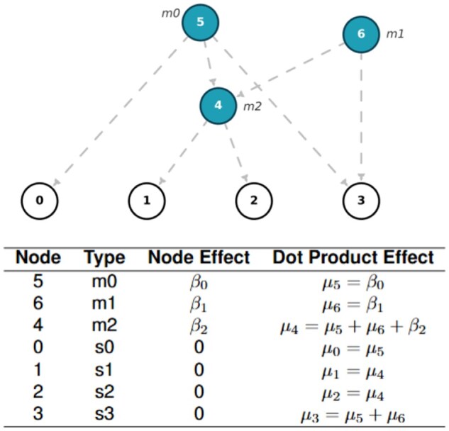 Figure 1
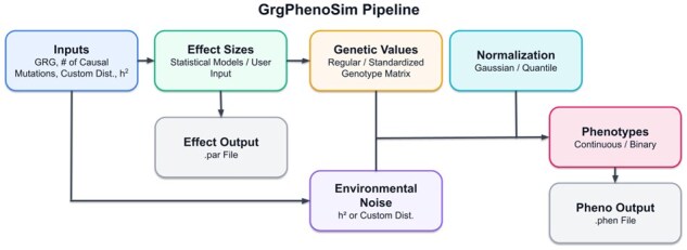 Figure 2
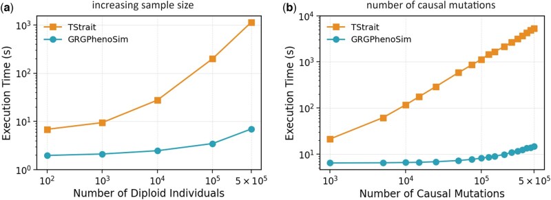 Figure 3
- —National Institutes of Health10.13039/100000002
Peer Reviews
No public reviews on file for this paper yet. If you reviewed it on a platform where reviews are public (OpenReview, ICLR, NeurIPS, ICML), you can paste yours below so the community can read it here.
Videos
No videos yet. Explain this paper in a talk, walkthrough, or lecture? Add one.
Taxonomy
TopicsGenetic Associations and Epidemiology · Genomics and Rare Diseases · Genetic and phenotypic traits in livestock
1 Introduction
Phenotypes, such as height (continuous) or type II diabetes (binary), refer to observable traits of an individual. Genome-wide association studies (GWAS), fine mapping, and heritability analysis are important for understanding the genetic architecture of phenotypes. Phenotype simulation is a pivotal part of these applications because it provides a ground truth for testing and evaluating new statistical methods. Causal variants are genetic variants that affect phenotypic values. Within the scope of phenotype simulation, causal variants are often sampled from genotype data, and then the phenotypes are computed based on the genotypes. Conventionally, such simulations use tabular genotype data structures such as the variant call format (VCF) (Danecek et al. 2011) and the PLINK (Chang et al. 2015) BED file format as input. However, as genotype datasets are becoming larger and larger, e.g. storing 200 000 phase UK Biobank whole-genome polymorphisms in VCF.gz (gzip compressed VCF files) requires 2.13 terabytes, it becomes increasingly expensive to perform repeated phenotype simulations on tabular genotype data (DeHaas et al. 2025).
An ancestral recombination graph (ARG) is a data structure that provides an efficient summary of the ancestry of population-level genetic data through coalescence and recombination events (Nielsen et al. 2025). ARGs can compactly store local genealogies along the genome that show how genetic materials have been recombined and inherited over time. Some ARG data formats, such as the tree sequence (TS) in tskit format (Kelleher et al. 2018), can also represent genotype data. The Python library tstrait (Tagami et al. 2024), building on this format, enables more efficient simulation of phenotypes than simulations based on tabular genotype data. Other existing phenotype simulators are insufficient for biobank-scale phenotype simulation because they either assume that the entire genotype dataset can be loaded into memory (Meyer and Birney 2018, Fernandes and Lipka 2020), which is unrealistic, or rely on sequential chunk-based loading (Wharrie et al. 2023), which is cumbersome. However, ARG inference is currently infeasible (or extremely expensive) for biobank-scale whole-genome sequencing (WGS) datasets, which have tens of times more variants than imputed data, thousands of times more variants than genotyping array data, hence limiting the utility of tstrait (Tagami et al. 2024) on real datasets.
Here, we leverage the genotype representation graph (GRG) (DeHaas et al. 2025) as the input to perform graph-based phenotype simulation. A GRG is a multi-tree structure that losslessly encodes the hard-call information in phased genotypes. The graph hierarchy efficiently represents information without using any compression library. Constructing GRG files for all autosomes of the 200 000 UK biobank WGS dataset cost a total of 80 pounds on the UK Biobank DNANexus cloud computing platform, yielding an uncompressed GRG that is 13 times smaller than the same dataset in compressed VCF (VCF.gz) format (DeHaas et al. 2025). Moreover, the dot product calculation via traversing over a GRG runs faster than all tested alternatives [PLINK (Chang et al. 2015), XSI (Wertenbroek et al. 2022), and Savvy (LeFaive et al. 2021)] and enabled extremely efficient GWAS (DeHaas et al. 2025). Here, we leverage GRG and its dot product function to build a highly efficient phenotype simulator to facilitate statistical method development. Moreover, we demonstrate the use of linear algebra operations on the standardized genotype matrix (an implicit transformation of the GRG), showing that the GRG dot product can be leveraged to speed up other statistical and population genetics calculations beyond phenotype simulation.
2 Methods
2.1 Model
2.1.1 A brief overview of GRG
A GRG (DeHaas et al. 2025) is a directed acyclic graph with nodes that contain zero or more “mutations.” In real data, the mutation status is often unknown, in which case either the derived allele or the minor allele can be used as “mutation.” The sample nodes correspond to the leaf nodes of the graph, which have no successors. Each haploid genome is represented as one sample node and each diploid genome is represented as two sample nodes. A path from the node containing mutation to the sample node exists if and only if the genotype for contains mutation , therefore encoding the same information as tabular genotype hard calls. A GRG (DeHaas et al. 2025) has down edges that are directed from the roots to the sample nodes (Fig. 1), and these edges carry forward the mutations down the tree.
A demonstration of GRG traversal for computing dot product values for phenotype simulation. The upper image shows a GRG, with node identifiers labeled within each node, and mutation identifiers labeled alongside their associated nodes. Every node in the GRG corresponds to a unique set of samples a node can reach, with individual mutations being associated with specific nodes. For instance, node 4 has two children—nodes 1 and 2, meaning that m2 (associated with node 4) is carried by nodes 1 and 2, but not by nodes 0 and 3. Finally, pairs of haploid sample nodes combine to form a single diploid sample (node 0 and 1 form the genotype for a hypothetical individual 1). The table below shows the graph traversal order and the corresponding dot product value at each node. In the context of phenotype simulation, node effect (input to dot product) is simply the causal phenotypic effects from the associated mutations with that node. The dot product function computes the dot product effect at a node by adding the dot product effects from all its parent nodes with its own node effect. For the sample nodes 0,1,2,3, the dot product effects (function output) are the genetic values of these corresponding haploid genomes.
2.1.2 GRG construction
A GRG can be obtained in two ways: (i) by constructing it directly from raw genotype data or (ii) by converting it from an ARG. Currently, GRG construction from raw genotype data can be performed using VCF, VCF.GZ, and IGD [indexable genotype data; DeHaas and Wei (2025)] formats using the command “grg construct” in GRGL. The GRG construction from IGD is the fastest. For example, constructing GRG for 200 000 UK Biobank samples using GRGL (v1) requires on average a few hours each chromosome on a DNANexus cloud node with 72 CPU threads (DeHaas et al. 2025). Alternatively, a GRG can be generated by converting an ARG stored in tskit TS format (Kelleher et al. 2016) using the “grg convert” command. This conversion takes less than a few minutes using a single CPU thread even for large sample sizes (DeHaas et al. 2025). A GRG directly converted from simulated TS is typically smaller than a GRG constructed from raw genotype data, leading to even faster downstream computation. In this study, we used GRGs constructed directly from raw genotype data when comparing against simulated TS, to provide a conservative benchmark.
2.1.3 Efficient matrix-vector operations with GRG
As discussed, each node within the GRG is mapped to one or more mutations (DeHaas et al. 2025). The mutations contained within the sample nodes are the cumulative effect of the mutations contained within all ancestral nodes. In order to compute genetic values for these samples, a graph traversal is necessary to ensure that the effect sizes are passed down through all ancestral nodes, right until the samples. The dot product operation in the GRG Library (GRGL) utilizes a highly optimized graph traversal method to compute the equivalent dot product result (DeHaas et al. 2025), such that matrix algebra operations can be easily implemented.
More specifically, let be a haploid (phased) genotype matrix of size 2 N-by-M, where N is the number of diploid individuals/genomes, and M is the number of variants. Each element in takes a value 0 or 1. Traversals of the GRG that only sum the values calculated transitively for each node’s children (upward traversal) are equivalent to the matrix product , where can be any 2 N-by-1 real vector. Similarly, traversals that only sum values calculated transitively for parents (downward traversal) are equivalent to the matrix product , where can be any M-by-1 real vector (Fig. 1). With the newly updated GRGL Python API v2.2, both types of dot products can be done efficiently via the function pygrgl.dot_product() (Wei Lab 2025).
2.1.4 Computing the additive genetic value
Let be a diploid genotype matrix of size N- by-M, such that each entry of can take a value of 0, or 1, or 2. Dot products involving or could be done via GRG by identifying mathematically equivalent operations based on the dot products involving or , because the additive (i.e. linear) relationship holds at each entry with row index i column index j.
The standard equation for computing continuous phenotypes under an additive genetic model is: . Here, is the N-by-1 phenotype vector, and designates the N-by-1 environmental noise vector. is the M-by-1 effect size vector, where entries corresponding to the causal variants that have nonzero causal effects and entries corresponding to non-causal variants are set to zero. We then call the pygrgl.dot_product() function to compute to get the additive genetic value for each haploid genome (Fig. 1). Adding the genetic values at the th and 2ith haploid genomes together, we get the ith diploid individual’s genetic value (Fig. 1).
2.1.5 Enabling standardized genotype matrix
Standardized genotype matrices are frequently used in statistical genetics. In GrgPhenoSim, we provide the option “standardized” for simulating phenotypes based on standardized diploid genotype matrix , where . Here, is an N- by-M matrix where each entry in the ith column is , twice the frequency of the mutation allele i. is a diagonal matrix where each ith diagonal element is the inverse standard deviation at a mutation, , with .
Briefly, in order to efficiently compute the genetic value , we calculate . Here, is a M-by-1 vector with elements at each ith entry. Therefore, can be computed via dot product between matrix and vector . After that, we perform an element-wise subtraction by , because is simply a N-by-1 vector filled with the same scalar that takes the value .
When the “standardized” option is evoked, the causal effect sizes are by default sampled from a normal distribution , where is the number of causal mutations, and is the narrow sense heritability. Then, after computing genetic value , environmental noise is sampled from to ensure that heritability is equal to .
2.2 Computational pipeline
The simulation pipeline processes GRGs through four main steps to generate phenotype data. The implementation utilizes numpy (Harris et al. 2020) for numeric operations (enabling standard math libraries such as BLAS) and pandas (Pandas Development Team 2020) for data manipulation and output. The pipeline (Fig. 2) starts with simulating causal effects, then proceeds with computing genetic values, adding environmental noise, and normalizing phenotypic values.
Visualization of the simulation pipeline.
The first step involves obtaining effect sizes for mutations in the GRG. Users can either use one of the built-in distributions or input custom effect sizes. The built-in statistical distributions include normal, exponential, fixed, gamma, and t-distributions, available for both univariate and multivariate (for jointly simulating multiple phenotypes) settings. When “standardized” genotype matrix is evoked, normal distribution will be used for simulating causal effect size. The dataframe contains the mutation_id, effect_size, and causal_mutation_id.
The second stage is to compute genetic values for diploid genomes, leveraging GRG dot product function (DeHaas et al. 2025) (Fig. 1). The system generates dataframes first at the sample level (sample_node_id, genetic_value, causal_mutation_id), and then at the individual level (individual_id, genetic_value, causal_mutation_id). Users may opt for normalizing genetic values at this stage.
The integration of environmental noise forms the third step, where the noise is generated through either an input narrow-sense heritability or a user-defined distribution. If using an input , when “standardized” genotype matrix is evoked, otherwise with the original genotype matrix . This stage produces a dataframe containing causal_mutation_id (for multiple causal mutations), individual_id, genetic_value, environmental_noise, and phenotype values.
The final optional normalization step offers either standard normalization or quantile normalization. Users can normalize either phenotypes alone or both genetic and phenotype values. For quantile normalization, the output dataframe includes all previous columns plus normalized_phenotype.
2.3 Additional features
GrgPhenoSim supports binary phenotype simulation. This step follows the standard pipeline to simulate a standardized continuous phenotype, then uses a population_prevalence parameter to establish a Gaussian threshold to convert continuous values into binary outcomes. Lastly, the system overwrites continuous phenotypes with their binary counterparts.
Further, GrgPhenoSim can accommodate multiple GRG inputs simultaneously, particularly useful when chromosome-specific genotype files are available, without having to merge them into a single file. This functionality requires consistent sample orders across GRGs and offers both parallel and sequential loading options. Genetic values from multiple GRG inputs are combined prior to noise simulation and final phenotype computation.
GrgPhenoSim can output standard .par files same as GCTA containing columns for mutation_id, AlternateAllele, Position, RefAllele, Frequency, and Effect (Yang et al. 2011). It can also output standard .phen files (Yang et al. 2011) containing person_id and phenotypes columns, with customizable header options.
This comprehensive pipeline (Fig. 2) ensures efficient phenotype simulation while being highly adaptable to individual users’ needs.
2.4 Usage
GrgPhenoSim is implemented and wrapped in Python and uses functionalities from the GRG library written in C++ to ensure efficiency. GrgPhenoSim offers two primary usage patterns: step-by-step execution through sequential notebooks, or a streamlined wrapper method for end-to-end simulation. A minimal example for continuous phenotype simulation is provided to showcase the simplicity of the Python interface.import pygrglfrom grg_pheno_sim.phenotype import sim_phenotypesgrg = pygrgl.load_immutable_grg(“example.grg”)phenotypes = sim_phenotypes(grg, heritability=0.3)
3 Results
3.1 Validation
Intermittent outputs were verified to ensure that the simulator works properly. For example, the GRG dot_product function was verified by testing against a recursive algorithm based on GRG, and against matrix multiplication based on the original genotype matrix. The genetic values computed by GrgPhenoSim were also cross-verified against tstrait (Tagami et al. 2024). In this validation, simulated TSs were converted to GRGs using GRGL. Identical effect sizes were fed into both GrgPhenoSim and tstrait (Tagami et al. 2024), and the resulting genetic values (i.e. ) were identical.
3.2 Runtime efficiency
We benchmarked the scalability of GrgPhenoSim against the current state-of-the-art graph-based phenotype simulator tstrait (Tagami et al. 2024), with respect to sample size and number of causal mutations (Fig. 3). The tests were carried out using a single thread on a compute node with x86_64 architecture, powered by an AMD EPYC 7763 64-Core Processor. A simulated dataset was used to create the GRGs used in the runtime experiments. We used msprime (Baumdicker et al. 2022) to simulate Mbp sequences for up to 500 000 diploid individuals (1 000 000 haploid samples) with a human-like parameter setting (effective population size , recombination rate , mutation rate ) (DeHaas et al. 2025). The GRGs were constructed from simulated VCFs. However, the corresponding TSs compared against the GRGs were simulated TSs.
Runtime efficiency tests. The two panels show runtime scaling with (a) increasing sample size and (b) number of causal mutations, illustrating the widening gap between GrgPhenoSim (in circles) and tstrait (in squares) runtimes.
3.2.1 Scaling with sample size
For this experiment, GRGs with 100, 1000, 10 000, 100 000, and 500 000 diploid individuals were used. The corresponding TSs were used to run the experiments for tstrait (Tagami et al. 2024). We used 100 000 causal mutations across all the tests.
Overall, we observed a gradual runtime scaling for GrgPhenoSim and a steeper scaling for tstrait (Tagami et al. 2024), as shown in exhibit (a) in (Fig. 3). Further, GrgPhenoSim was significantly faster regardless of the sample size used, with the gap in runtime widening as the sample size increased. At 500 000 individuals, GrgPhenoSim was 162× faster than tstrait (Tagami et al. 2024).
3.2.2 Scaling with number of causal mutations
For this experiment, the constructed GRG and the corresponding TS for 500 000 diploid individuals were used, with a total of 575 054 mutations in the dataset. The number of causal mutations ranges from 1000 to 500 000.
Once again, we observed a gradual runtime scaling for GrgPhenoSim and a steeper scaling for tstrait (Tagami et al. 2024), as shown in (Fig. 3b). Moreover, GrgPhenoSim was significantly faster for every dataset, and the run-time gap widened as the number of causal mutations increased. At 500 000 causal mutations, GrgPhenoSim was 587 times faster than tstrait (Tagami et al. 2024). When simulating 10 000 causal variants, it takes up to 5 s to run GrgPhenoSim for each of the 22 autosomes for 3202 samples in the 1000 Genomes Project (Byrska-Bishop et al. 2022).
4 Discussion
GrgPhenoSim provides a flexible and efficient interface to simulate phenotypes using GRGs. Taking advantage of the computational speed up from the GRG data structure and wrapping it into simple Python functions, it provides users with the ability to efficiently simulate phenotypes without having to understand the GRG data structure. While GrgPhenoSim is faster in all tested settings, the run time advantage becomes even more significant when the sample size is large, which is when repeated phenotype simulations are costly with existing methods. Converting an ARG from a tskit TS into a GRG (TS-GRG) takes only seconds to a few minutes (DeHaas et al. 2025). Thus, when a simulated or inferred TS is already available, generating a TS-GRG can still be advantageous for downstream analyses—such as phenotype simulations—that do not require the full information content of the ARG.
GrgPhenoSim is currently the only phenotype simulator that operates directly on GRGs, further expanding and strengthening the GRG computational ecosystem. Together with the GWAS function in GRGL and GRG dot_product, GrgPhenoSim could facilitate the development of statistical genetic methods for biobank-scale datasets, enabling a wider range of GWAS-related applications using GRG functionalities. Last but not least, we demonstrated that GRG dot product can be used to speedup calculations involving standardized genotype matrices, which could facilitate future GRG-based statistical genetics.
The reference list from the paper itself. Each links out to its DOI / PubMed record.
- 1Baumdicker F , Bisschop G, Goldstein D et al Efficient ancestry and mutation simulation with msprime 1.0. Genetics 2022;220:iyab 229.34897427 10.1093/genetics/iyab 229PMC 9176297 · doi ↗ · pubmed ↗
- 2Byrska-Bishop M , Evani US, Zhao X et al High-coverage whole-genome sequencing of the expanded 1000 Genomes Project cohort including 602 trios. Cell 2022;185:3426–40.e 19.36055201 10.1016/j.cell.2022.08.004PMC 9439720 · doi ↗ · pubmed ↗
- 3Chang CC , Chow CC, Tellier LC et al Second-generation plink: rising to the challenge of larger and richer datasets. Gigascience 2015;4:7–015.25722852 10.1186/s 13742-015-0047-8PMC 4342193 · doi ↗ · pubmed ↗
- 4Danecek P , Auton A, Abecasis G et al; 1000 Genomes Project Analysis Group. The variant call format and vcftools. Bioinformatics 2011;27:2156–8.21653522 10.1093/bioinformatics/btr 330PMC 3137218 · doi ↗ · pubmed ↗
- 5De Haas D , Wei X. Igd: a simple, efficient genotype data format. Bioinform Adv 2025;5:vbaf 205. 10.1093/bioadv/vbaf 20540980555 PMC 12448908 · doi ↗ · pubmed ↗
- 6De Haas D , Pan Z, Wei X. Enabling efficient analysis of biobank-scale data with genotype representation graphs. Nat Comput Sci 2025;5:112–24.39639156 10.1038/s 43588-024-00739-9PMC 12054550 · doi ↗ · pubmed ↗
- 7Fernandes SB , Lipka AE. simplephenotypes: simulation of pleiotropic, linked and epistatic phenotypes. BMC Bioinformatics 2020;21:491.33129253 10.1186/s 12859-020-03804-y PMC 7603745 · doi ↗ · pubmed ↗
- 8Harris CR , Millman KJ, van der Walt SJ et al Array programming with Num Py. Nature 2020;585:357–62. 10.1038/s 41586-020-2649-232939066 PMC 7759461 · doi ↗ · pubmed ↗