Ensemble Effects on Hydroxide Bond Dissociation Free Energies in Polyoxovanadate Clusters
Andreas Towarnicky, John N. El Berch, Giannis Mpourmpakis

TL;DR
This paper shows how considering molecular ensembles improves predictions of hydroxide bond energies in vanadium clusters, aligning theory with experiments.
Contribution
The study introduces a bilinear model and methodology that captures ensemble effects, reducing DFT calculations by 98% while maintaining high accuracy.
Findings
Ensemble effects significantly influence hydroxide bond dissociation free energies in polyoxovanadate clusters.
A bilinear model reconciles experimental and theoretical results with a root-mean squared error of 0.4 kcal/mol.
A simplified methodology achieves 1 kcal/mol accuracy with 98% fewer DFT calculations.
Abstract
Understanding structure-property relationships is foundational to numerous modern chemistries, such as proton-coupled electron transfer (PCET). However, an experimentally measured property is the result of the behavior from an ensemble of molecules. Neglecting ensemble effects, especially under complex chemical environments, may obfuscate these relationships and lead to discrepancies between theory and experiment. In this work, we demonstrate the impact of configurational entropy and local chemical environments on hydroxide bond dissociation free energies [BDFE(O–H)] for a set of polyoxovanadate nanoclusters, at ambient conditions. The O–H bond strengths are investigated via density functional theory (DFT) coupled with statistical thermodynamic analysis and bilinear modeling, and compared with previous experimental results on the same systems, namely electrochemical solutions of:…
Genes, proteins, chemicals, diseases, species, mutations and cell lines named across the full text — each resolved to its canonical identifier and authoritative record.
Click any figure to enlarge with its caption.
 1
1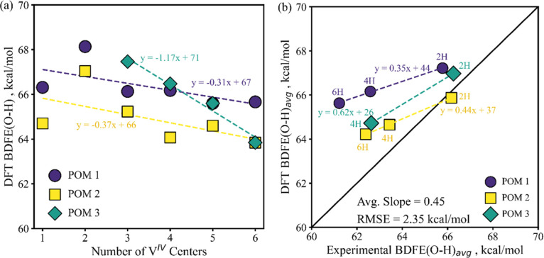 2
2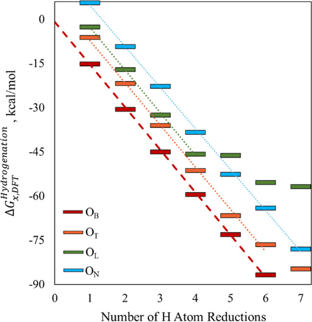 3
3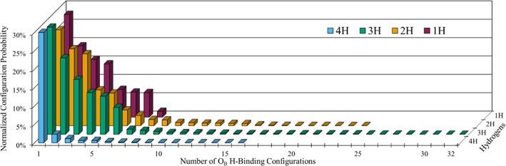 4
4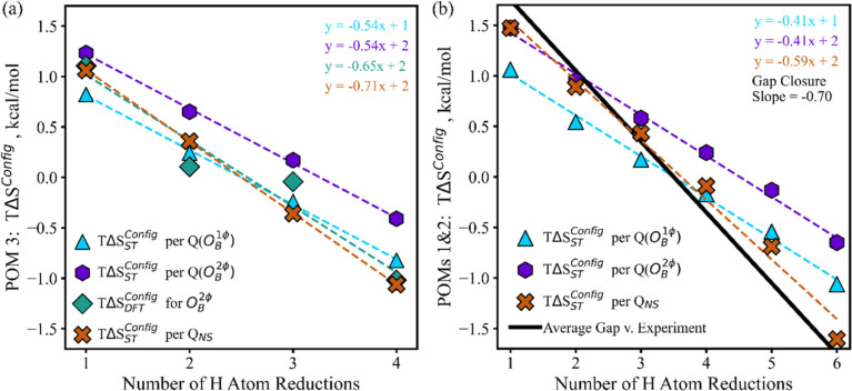 5
5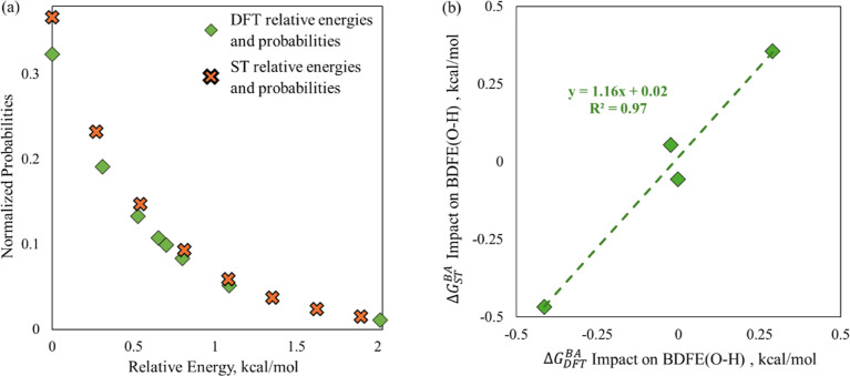 6
6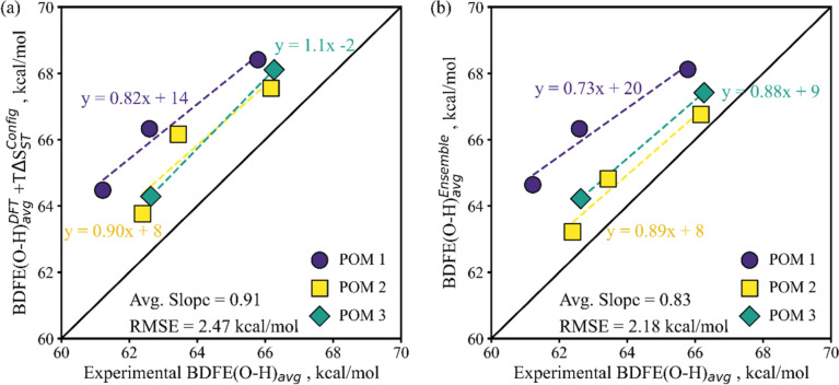 7
7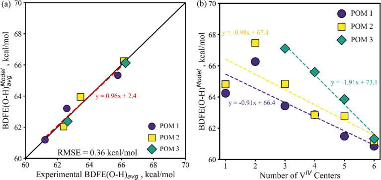 8
8- —Basic Energy Sciences10.13039/100006151
Peer Reviews
No public reviews on file for this paper yet. If you reviewed it on a platform where reviews are public (OpenReview, ICLR, NeurIPS, ICML), you can paste yours below so the community can read it here.
Videos
No videos yet. Explain this paper in a talk, walkthrough, or lecture? Add one.
Taxonomy
TopicsPolyoxometalates: Synthesis and Applications · Metalloenzymes and iron-sulfur proteins · Vanadium and Halogenation Chemistry
Introduction
1
Advancing modern technologies requires fundamental understanding of complex phenomena, including PCET, ?,? and their manifestations in gainful systems such as metal oxides? and polyoxometallates (POMs). ?−? ? PCET is equivalent to hydrogen atom transfer (HAT) when colocated and concerted, ?,? and by the natural ubiquity of hydrogen, is thus central to a large number of chemical reactions ?−? ? ? ? as well as their catalysis. ?,?,? Although fundamental, challenges remain to elucidating PCET at ensemble scales, ?,? including significant computational expense and lingering gaps between theory and experiment. Metal oxides participate in many PCET applications, and offer the ability to tailor PCET mechanisms? while providing versatility, structural stability, and tunable? physicochemical properties. POMs are atomically precise metal oxide clusters with similar surface bonding motifs to extended metal oxides, thus, bridging molecular to extended systems. ?,? These advantages make POMs ideal systems to investigate PCET chemistries, improve understandings, and hone computational approaches.
A key descriptor of PCET is the bond dissociation free energy, ?−? ? ? and specifically with POMs, the hydroxide BDFE(O–H). ?,? BDFE(O–H) values describe the homolytic cleavage of an H atom, and are thermodynamically equivalent to successive electron and proton transfers, in either order, which comprise the overall reaction. ?,? Therefore, changes in the electron affinity or basicity of POMs can influence the BDFE(O–H), which further connects to PCET kinetics via Marcus theory. ?,?,? Understanding of the various influences on BDFE(O–H) and thus PCET, is central to electrocatalytic chemistries such as the oxygen reduction reaction (ORR).?
Previous investigations have provided substantial understanding of various aspects of POM chemistries. Work by Maeda et al. determined that more negative POM cluster charges effect more negative electrochemical reduction potentials? (less exergonic electron affinities). Changes in electron affinity translate directly to changes in BDFE(O–H) if the proton transfer energetics remain the same, and have been shown to manifest in POM-catalyzed chemistries.? Similarly, changes to POM constituent metals were demonstrated to affect POM reduction potentials ?,?−? ? and BDFE(O–H) in alignment with the energetics of reducing the metal centers.? Different POM morphologies were previously shown to influence different site-specific basicities,? which were revealed to extend to morphology-dependent and site-specific BDFE(O–H).? Solvation effects on small molecule BDFE(O–H) have generally been found to be minor, ?,? but can be substantial with POMs if specific interactions contribute to coordination-induced bond weakening.? Functionalization of POMs with different ligands has been illustrated to modify their reduction potentials.? In our recent work we demonstrated that changes in ligand identity (Figure), such as their electron-withdrawing or donating nature, can change POMs electron affinity.? Although this effect may be largely offset in their impact on BDFE(O–H) by concomitant changes in basicity,? a phenomena known as thermodynamic compensation. Additionally, this work further demonstrated an increase in electronic communication across the Lindqvist core due to surface methylation, ?,? and that BDFE(O–H) was strongly influenced by the charge transfer to the bridging oxygen atoms.? However, a moderate degree of offset was present between the experimental and computationally derived BDFE(O–H) values (Figureb, vide infra), and the changes in BDFE(O–H) effected by successive H atom reductions were incompletely captured by theory.?
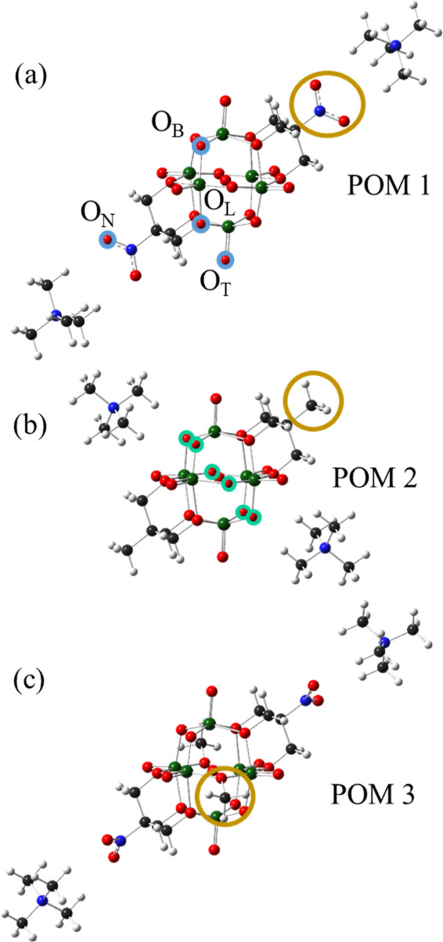
DFT geometrically optimized structures of: (a) [Me4N]2[V6O13(TRIOLNO2 )2] (POM 1), (b) [Me4N]2[V6O13(TRIOLMe)2] (POM 2), and (c) [Me4N]2[V6O11(OMe)2(TRIOLNO2)2] (POM 3). Functionalization of POM 1 with two surface methyl groups results in POM 3 in (c). Atom Key (spheres): green, V; red, O; black, C; blue, N; white, H. Brown circles indicate different functionalization of POMs: nitro-functionalized TRIOL ligands in POM 1, methyl-functionalized TRIOL ligands in POM 2 and surface methylation in POM 3. Blue circles on POM 1 indicate different possible H-binding oxygen sites, Bridge (OB), Terminal (OT), Ligand (OL), and Nitro (ON); the center internal oxygen is not surface accessible. Green circles on POM 2 indicate the six thermodynamically favored OB–H binding sites (analogous to the 6 OB of POM 1). POM 3 has only 4 OB atoms available.
(a) DFT BDFE(O–H) x of each POM, where x = 1–6 for POMs 1 and 2, corresponding to the same number of VIV centers, and x = 1–4 for POM 3, corresponding to 3–6 VIV centers; and (b) parity plot of DFT vs experimental BDFE(O–H)avg. The POM trends of (a) are plotted vs the number of VIV centers to show the values at the same cluster oxidation states. These represent the same data published in our previous work with the Matson group.
Improved understanding is key to close residual theory-experiment gaps and enable greater accuracy and efficiency from first-principles calculations. To this end it is instructive to consider the atomically precise systems of our prior work? in greater detail. Specifically, in collaboration with the Matson lab, we compared experimentally measured 2H atom average BDFE(O–H)avg with corresponding values calculated via DFT.? DFT satisfactorily corroborated the experimentally observed trend of decreasing BDFE(O–H) with increasing degree of H atom reduction to the POMs (see the BDFE(O–H) slopes of Figure, vide infra), but DFT underestimated the trend by about half, and point-specific differences of 1 to 4 kcal/mol were present. The incomplete trend-capture result is similar to previous findings by Agarwal, Kim, and Mayer,? who noted that the change in BDFE(O–H) upon increasing H atom reduction of mixed valence ceria nanoparticles (Ce^3+^/Ce^4+^) could not be satisfactorily explained with Nernstian mass-action or Langmuir chemisorption models. In fact, on their 2–4 nm nanoparticles with on the order of 100 potential binding sites, they found that these models would underestimate the BDFE(O–H) changes by an order of magnitude (more than 10 kcal/mol), highlighting the significance of the degree of metal center reduction by H atoms. In our POM systems,? DFT provided improved trend-capture, attaining ∼50% compared to ∼20% by Nernstian analysis.? However, the remaining BDFE(O–H) differences between theory and experiments are sufficient to eclipse other effects (e.g., differences in ligation), and suggest that further theoretical consideration may be beneficial.
Two possible areas for greater examination are discerned from considering the nature of molecular DFT calculations and the experiments themselves. The experiments in our prior work? were on electrochemical solutions, with millimolar POM concentration, organic acid, and buffers, and their BDFE(O–H) values entail the measurement of POM interaction with the electrode surface and its boundary layers.? In our previous investigations, DFT considered individual POM structures and thus did not account for ensemble effects that may be present in solution, particularly among energetically accessible POM isomers. The DFT calculations also do not account for how the complex chemical environment may affect POM BDFE(O–H). Our prior work further illustrated a significant impact of the electronic environment on BDFE(O–H) in relation to the POM bridging oxygen (O_B_) charges.? We hypothesize that considering these aspects may help resolve gaps between experiment and theoretical calculations.
Initial inspection of the POM structures with regard to the number of possible POM O–H binding sites (Figure, vide infra) suggests that a configurational entropy factor S ^Config^ may be on the order of 1 to 2 kcal/mol per H binding, which is commensurate to the discrepancy between the computational and experimental BDFE(O–H) trends. Considering insights from the hydrogenation of metal oxide extended surfaces, Fripiat and Lambert found that S ^Config^ and averaging across different site energies (affording a difference vs the minimum site energy, herein termed ΔG ^BA^) were key in fitting theory to experimental adsorption isotherms,? and additionally that the S ^Config^ could be determined via sterically informed statistical thermodynamics. Furthermore, the S ^Config^ contribution to Langmuir adsorption isotherms is generally known? and may be inferred to extend to chemisorption. Various studies by our group ?,? and others ?−? ? have shown how considering ensemble effects can improve the prediction of thermochemical properties and catalyst behavior. However, additional multiscale modeling efforts, such as incorporating MonteCarlo sampling, are often required to resolve S ^Config^ and ensemble effects, ?,? and their resolution via DFT may be impractical for combinatorially complex systems. Notwithstanding challenges via other methods, and noting the atomically precise POM structures and previous connection to O_B_ charges, we were motivated to explore whether ensemble effects and the electronic environment could be accounted for via statistical thermodynamics and linear incorporation of an atomic charge factor, respectively.
To the best of our knowledge, the role of ensemble effects in POM hydrogen transfer energetics has yet to be described, especially through fundamental statistical thermodynamics and structure-function relationships. In this work we demonstrate how the presence of multiple, near-equivalent hydrogen-binding sites on POMs give rise to ensemble effects on subnanoscale oxide systems that can affect the calculated POM property (herein, BDFE(O–H)). Further, we demonstrate that accounting for the local chemical environment via bilinear modeling with O_B_ charges may close systemic offsets between theory and experiment. Overall, we introduce new computational avenues for rapid calculations of BDFE(O–H) values, leading to improved accuracy in modeling POMs and similar systems.
Computational Methods
2
Density Functional Theory
2.1
DFT calculations were performed using the Gaussian 16 program package.? The hybrid functional B3LYP? was used together with the LANL2DZ basis set,? which afforded computational efficiency while maintaining accuracy.? Implicit solvation was utilized via the self-consistent reaction field with acetonitrile as solvent, corresponding to the experiments? [SCRF = (SMD,acetonitrile)].? This level of theory resulted in very good agreement between theory and experiments in describing BDFE(O–H)avg trends on polyoxovanadates? and polyoxotungstates.?
DFT geometrically optimized structures with counterions are illustrated in Figure for the same POMs as investigated experimentally.? DFT calculations utilized tetramethylammonium counterions instead of the tetra(n-butyl)ammonium used in experiments? to reduce computational cost. All structures were fully optimized to standard tolerances (RMS force ≤ 3 × 10^–4^ hartree per Bohr)? or even tighter criteria. Vibrational frequencies were computed for the optimized geometries. ?,? confirming the energy minima to be free of imaginary frequencies. The DFT-optimized structures matched those previously resolved via XRD with great agreement.? Thermochemical values were determined at 298.15 K and 1 atm, ?,? corresponding to experimental conditions.? Natural Bond Orbital (NBO)? analysis was used to calculate atomic charges. Atomic visualizations were developed with GaussView 6.?
Gibbs free energy values were used to compare relative energetics of different configurations and spin states. Elevated spin states were evaluated for each hydrogen binding configuration investigated, up to a multiplicity corresponding to (#V^IV^ + 2) unpaired electrons, where #V^IV^ is the number of reduced vanadium atoms (e.g., [V_6_O_9_(OCH_3_)2(OH)2(TRIOL^NO2^)2]^−2^ has 4 V^IV^ centers and all spin states were investigated up to a multiplicity of septet). Beyond the multiplicity corresponding to #V^IV^ unpaired electrons, a significant increase in calculated energy was invariably observed (Figure S1). In these structures, no significant spin contamination was noted. For each degree of H atom reduction, the lowest energy combination of spin state and H-binding configuration was utilized for BDFE(O–H) calculations.
To find the lowest energy DFT structures, for each degree of H-binding we considered incremental configurations (adding 1H at a time) to each of the available oxygen atoms, i.e. considering at least one incremental configuration for all Bridge, Terminal, Ligand, and Nitro oxygen (O_B_, O_T_, O_L_, and O_N_, respectively) (Figurea, blue circles). For each 1H increment, the lowest energy configuration was retained for the next 1H evaluation. Two orientations of O–H dihedral angle are possible for each O_B_–H binding (Figure S2a). For POMs 1 and 2, considering all possible combinations with both O_B_–H configurations becomes computationally prohibitive, requiring at least 2005 DFT geometry optimizations and vibrational analyzes for each POM (Table S1). Thus, for POMs 1 and 2, only O_B_–H combinations with the same direction of OV–O–H dihedral angle were considered (i.e., all configurations with all O–H pointing the same direction, minimizing steric hindrance. e.g. Figure S2b). For POM 3 with only 4 O_B_, it is computationally viable to consider all possible O_B_–H combinations with both dihedral angle directions, as only 250 calculations are required (Table S1). Herein we term these sets as O_B_ ^1φ^ limited to just one dihedral angle direction, and O_B_ ^2φ^ considering both dihedral directions. All three POMs were evaluated through 7 total degrees of reduction, considering both H atom reduction and alkylation (e.g., 5H + 2CH_3_ for POM 3).
The results reported herein focus on the thermodynamically preferred O_B_ H-binding sites, which are the same series of structures and resultant BDFE(O–H) values previously reported.? The structures are utilized subsequently for comparison purposes, statistical thermodynamic analysis, and bilinear modeling. In similar fashion as described above, select additional series of structures were resolved to provide more complete statistical thermodynamic representation of H-binding (particularly for POM 3), and we considered different counterion identities and/or coordinations (Figure S3). BDFE(O–H) values were calculated from the DFT results by the following eqs–?
Where G stands for the Gibbs free energy, in kcal/mol. G corr includes thermal internal energy, enthalpy, zero-point energy correction, and entropies from translation, rotation, vibration, per Gaussian Thermochemistry.? The DFT BDFE(O–H) and BDFE(O–H)avg may be calculated directly per eqs and ? below, using the lowest free energy configurations. Note that our experimental points of comparison are all BDFE(O–H)avg values, determined from pairs of clusters on the basis of 2H increments.? Here G ^H^•^ ^ refers to the Gibbs free energy of the solvated hydrogen atom, and all components are solvated unless otherwise stated.
here x = the number of H atom reductions of the cluster, and the G _ xH_ ^POM^ are the G DFT of the minimum-energy configurations for the respective degrees of H-binding. Equations and ? are the same as used in our previous work.? Corresponding hydrogenation energies on either incremental or cumulative basis are calculated per eqs and ?, respectively
Ensemble Thermodynamics
2.2
Ensemble effects include S ^Config^ and Boltzmann averaging (BA) across the free energies of a population, G ^BA^. Each degree of H-binding to a POM affords a population of possible configurations. The ensemble S ^Config^ and G ^BA^ for these populations depend on the relative energies of their constituent POM configurations, which are calculated per eq, and their state probabilities, which are determined per Boltzmann statistics, eq
here “i” refers to the distinct configurations (states) for the same degree of H-binding and p _ i _ is the normalized probability among all configurations with the same number of H-bindings, R is the gas constant, and T is the absolute temperature (298.15 K; room temperature). ΔG _ i _ ^rel^ is the relative Gibbs free energy between specific configuration “i” and the lowest energy configuration [min(G _ i _ ^POM^)]. We assume the Ergodic hypothesis holds and that the individual state probabilities are equal to their ensemble fractional populations. These probabilities may then be used to determine the S ^Config^, via the Gibbs entropy equation (eq) and the Boltzmann average G ^BA^ per eq
Equation is shown providing the Boltzmann average of the DFT values of the POM Gibbs free energies (G DFT ^BA^) taken across the absolute DFT free energies (G _DFT,i _ ^POM^) directly. Prior works by our group? and others ?−? ? ? ? note that to describe a complete ensemble, the contribution of S ^Config^ must be considered in addition to the DFT-calculated Gibbs free energies of individual structures. Thus, to account for the total free energy of a system, −TS^Config^ is incorporated as in eq
Here G Total ^BA^ is the Boltzmann average of the total Gibbs free energies of particles in the ensemble including the contribution of S ^Config^. We note that factoring the minimum energy structure of the ensemble, min. (G _DFT,i _ ^BA^), can be used to afford eq below. This allows us to proceed and consider separately the effects from S ^Config^, and ΔG ^BA^; where ΔG ^BA^ is the difference between the ensemble Boltzmann average DFT free energy (G DFT ^BA^) and the DFT minimum min(G _DFT,i _ ^POM^), where the lowest energy DFT structures correspond to the same BDFE(O–H) that were published in our previous work.?
This separation of terms is useful for subsequent thermodynamic analysis. Similarly, note that the ΔG _ i _ ^rel^ and p _ i _ per eqs and ? may be used to calculate ΔG ^BA^ directly
Statistical Thermodynamic Approximation of S
Config
2.3
Equations & ? may be used to calculate S ^Config^ and ΔG ^BA^ when the individual configurational probabilities (p _ i ) or energies (G _ i _ ^POM^) are known, i.e. when it is reasonable to resolve all relevant configurations via DFT. As noted above, this is achieved for POM 3 but is not practical for POMs 1 and 2 (Table S1). To determine the S ^Config^ and ΔG ^BA^ for POMs 1 and 2, we need to resolve representative distributions for their configurational free energies, for each degree of H-binding. Experience in prior work? suggested small but non-negligible energetic differences exist between different configurations with the same type of O–H site binding, i.e. between H-bindings to different O_B sites. Therefore, we considered approximating the ensemble of different configurations via Boltzmann statistics, affording exponential decay distribution functions per the configurations’ relative energies (vide infra Figures, ?a, and S10–S12). A continuous mathematical expression for the probabilities of states analogous to eq takes the form of?
Here y is used to distinguish from the discrete states denoted with i above. λ is the decay parameter that describes how sharp or wide the distribution is. Smaller λ leads to wider distributions, and larger values afford shaper distributions. The continuous form of eq suits substitution of p (y) into eq and integration across the continuous domain of y. This proceeds via eqs–?, and affords a tidy analytic expression for S ^Config^ per its distribution (eq)
The solution to this integral is
To further resolve these distributions, we need information about either S ^Config^, λ, or related quantities. As noted previously, for systems with large numbers of configurations such as POMs 1 and 2, it is impractical to solve them directly via DFT. However, the S ^Config^ and/or λ may instead be informed by the structural nature of H-binding to a POM, such as the possible numbers of configurations, and/or how those configurations affect the ensemble entropy.
From the above, one can deduce that as the number of relevant configurations in a distribution increases, the distribution grows wider, λ decreases, and S ^Config^ increases. Consistent with this behavior, it is well-known that for a system with isoenergetic (equiprobable) configurations, S ^Config^ can be approximated by?
Where Q E is the number of equiprobable configurations, i.e. the degeneracy. The subscript ST is used to denote that the value is approximated via statistical thermodynamics as opposed to DFT calculation. We note that the Boltzmann distributions describing our system (eqs and ?) represent canonical ensembles and/or canonically equivalent multicomponent microcanonical ensembles (MC_Micro) with some number of nonisoenergetic configurations, while isoenergetic states would comprise microcanonical state counting;? see Figure S4 for an illustration. However, we consider the limit in which the relevant number of configurations, Q, is restricted by the system temperature and nature of the distributions to a set of essentially degenerate, isoenergetic configurations. This is the case when some structural feature, e.g. presence vs lack of steric hindrance, creates an energetic difference between types of configurations, with system temperature sufficient to populate one type (i.e., with low energy) but not those with higher energy. Therein only one site type meaningfully characterizes the ensemble Gibbs free energy and changes to it (e.g., bridge site configurations without steric hindrance). Maintaining the number of particles, N, system volume, V, and energy, E, constant between MC_Micro and degenerate microcanonical ensembles requires that
where “i” refers to the energetically diverse components of an MC_Micro ensemble, which has equivalent components to a canonical ensemble (see illustration Figure S4). Both the MC_Micro and canonical ensembles fit the configurational distributions we are considering herein (eqs and ?). With this framework, equal E, N, and V across all three ensemble types implies that temperature, T, must also be equal, and that accordingly the ensembles will afford equivalent predictions for entropy, which is the case in the thermodynamic limit when accurately approximating the same macroscopic system. ?−? ? ? ? ? Thus, the microcanonical degeneracy in the effectively isoenergetic limit may be apportioned to a canonical distribution, as
Equivalent entropies follow mathematically, multiplying both sides by R. To justify the applicability of the thermodynamic limit, we note that we are working with experimental solutions having N on the order of 10^20^, that changes to the system size do not affect their intensive properties (i.e., extensive additivity holds), and that our systems are at equilibrium, have positive heat capacity, uniform phase, and are not near any phase transitions. ?,?−? ?,? Equivalent entropies enable us to consider eq equal to eq, affording
Solving eq affords
Here e is Euler’s number, approximately 2.71. Thus, if we determine a set of approximately isoenergetic configurations, Q E, we can describe the corresponding Boltzmann distribution and S ST ^Config^. With the Boltzmann configurational distributions now characterized by their entropies, we can consider them further to determine ΔG ^BA^.
Statistical Thermodynamic Approximation of
ΔG BA
2.4
To determine ΔG ^BA^, we could proceed via analogous continuous approximation of eq as we did with eq for S ^Config^. However, considering equivalent domains for p _ y _ and p _ i _, one notes that the exponent of eq (−yλ) is also equal to −ΔG y ^rel^/RT per eq. In integrating the analogous continuous form across the full domain of y (eq), the G _ y _ ^rel^ terms cancel, and the expression would just reflect the thermal energy in every case, with RT = 0.592 kcal/mol at the experimental conditions (298.15 K, 1 atm)
This may be satisfactory where Q is large, but not for systems where Q is small and the available states are further apart in energy such that higher energy states may not be visited. Thus, to determine the ΔG ^BA^, we instead consider a rediscretized distribution
Workup of eq is now aided per the above derivation that provides the λ values (eq). Here “j” is an index of states that runs from 0 to a satisfactorily large number, e.g. 10 × Q E, such that higher j would not significantly contribute to the ensemble population or average value calculations. The λ values parametrize the range over which j is relevant per eq. Additionally, using λ normalizes the functions consistently with the same Q E state-counting. With probabilities calculated per eq, ΔG ST ^BA^ may then be straightforwardly calculated per eq. With this practical framework in hand, we can now calculate ensemble S ^Config^ and ΔG ST ^BA^ contributions to BDFE(O–H) without excessive DFT requirements.
Bilinear Modeling of BDFE(O–H)
2.5
Bilinear modeling was performed with the StatsModels? Python module least-squares linear regression. Models with and without S ^Config^ and ΔG ^ΒΑ^ were considered. The bilinear interaction term was not found to be significant for these systems, and was thus precluded from the present models (coefficient set equal to zero). All final parameters were verified as significant (p < 0.01). All models were cross-validated with leave-one-out methods with respect to both individual BDFE(O–H)avg data points and POM sets of BDFE(O–H)avg.
Results and Discussion
3
DFT Insights to POM BDFE(O–H) Behavior
3.1
DFT investigation of 1H incremental H atom reductions, illustrated in Figurea, reveals values for the odd-numbered BDFE(O–H), which were not attainable experimentally.? These values help confirm the trend of decreasing BDFE(O–H) with increasing degree of cluster H atom reduction, and highlight the overall linearity of these trends (Figurea). An analogous plot of experimental BDFE(O–H)avg is provided in Figure S5 for comparison. In Figurea, the BDFE(O–H) trend clearly takes on similar slopes for POMs 1 and 2, suggesting that the BDFE(O–H) trend is not substantially affected by the electronic effects of the ligand identity. This is consistent with the phenomena of thermodynamic compensation noted in our earlier work.? Meanwhile, the sharper slope of POM 3 is made clear on a 1H basis (Figurea), further emphasizing another finding from our previous work, that the surface alkylation of POM 1 affording POM 3 has increased the magnitude of connection between the BDFE(O–H) and the degree of cluster H atom reduction.?
To fully consider the linearity of the DFT BDFE(O–H) trends, one notes in Figurea that the first BDFE(O–H) for POMs 1 and 2 are lower than the second. This could reflect an electronic symmetry factor previously observed by the Matson and Miró groups for the singly reduced POMs.? The relative symmetry of the non-hydrogenated cluster could stabilize it and thus reduce the first BDFE(O–H); while symmetry breaking with the first protonation could slightly destabilize the 1H cluster. Together with an unpaired electron for the 1H cluster, this could favor some pairing with a second H atom reduction, slightly increasing its BDFE(O–H). These findings suggest some impetus for these POMs to participate in PCET in 2H^+^/2e^–^ increments. This is consistent with previous findings on POM 1,? the slope of the Nernstian open circuit potentials,? and combination of experimental redox events into 2H^+^/2e^–^ PCET events. ?,? Taking the first two metal center reductions on their average, the remaining BDFE(O–H) points and trends suggest little deviation from linearity.
Figureb expands upon our previous work? by underscoring that while sufficient for corroboration, compared to experimental findings the raw DFT calculations captured only part of the BDFE(O–H) trend (45% on average) and exhibit an overall root mean squared error (RMSE) of 2.35 kcal/mol. Additionally, offsets vs parity are apparent on a per-cluster basis. This motivates our current work, and we demonstrate how ensemble effects (commonly neglected in DFT calculations) can give rise to deviations between experiments and theory.
First expanding the scope of DFT investigation from our prior collaborative work,? we considered additional H-binding configurations (Figure S2a and Table S1), counterion identities and positions (Figure S3). An overview of the different oxygen site energetics (lowest energy structures for the specific binding site types) is provided in Figure, displaying the cumulative energies of hydrogenation for incremental O–H binding positions. The different possible H-binding site types (Figurea, blue circles) correspond to different incremental energies of hydrogenation (Figure), which mostly remain consistent throughout full occupation of the O_B_. Consistent with our previous findings? Figures and S6 for POMs 2 and 3 illustrate that O_B_ sites are thermodynamically preferred, and that cluster hydrogenation is exergonic through full occupation of the available O_B_ sites (6 for POMs 1 and 2; 4 for POM 3), corresponding to 1-electron reduction of all initial V^V^ atoms. Additionally, Figures and S6 show that the incremental hydrogenation energies and their linear trends are substantially constant for cluster reductions up to 6 V^IV^.
Cumulative Gibbs free energies of hydrogenation with different incremental H-binding locations on POM 1, relative to the 0H cluster, per eq . The configurations for each successive H-binding are based upon the preceding lowest energy configuration.
These results are important for understanding prospective PCET energetics of bulk vanadium oxides, as the nanocluster vanadium-oxygen bond types are very similar to those found on bulk system surfaces.? Both molecular and bulk system surfaces feature O_B_ and O_T_ sites (Figures and S7) and may be analogously ligand-modified and/or hydrogenated. The incremental hydrogenation energies correlate to the BDFE(O–H) via eqs–?, which change in reference from 1/2H_2_(g) hydrogenation to solvated H atom reductions. O_T_ sites are consistently found to be second-most thermodynamically favored for H-binding, but at least 6 kcal/mol less favorable than O_B_ sites if O_B_ are available. An important consequence thereof is that the relative ensemble populations of O_T_–H and higher energy states at ambient conditions is much lower than O_B_ configurations, on the order of <50 ppm per eq. Similarly, the incremental hydrogenation energies beyond 6 V^IV^ in the clusters correspond to non-O_B_ sites and are much smaller, by at least 10 kcal/mol. Using different counterions or different counterion positions (Figure S3) did not substantially affect the hydrogenation trends. Considering variable counterion positions within a series was found to have only minor effect on incremental energies, <1 kcal/mol (Figure S8), attributed to minor differences in cluster-counterion interaction and OH-counterion steric hindrance. None of the variations considered significantly improved experimental BDFE(O–H)avg trend-capture.
Inspection of the individual DFT E Electronic and G corr terms reveals that the vast majority of the BDFE(O–H) and its trends with H atom addition arise from differences in E Electronic (Figure S9). These G corr values utilize standard harmonic analysis. ?,? Anharmonic vibrational analyzes were also considered to refine G corr, but for these POM systems, each anharmonic calculation required inordinately large computational resources and considering them across ensemble sets was found to be prohibitive. Moreover, anharmonic calculations would be expected to slightly lower G corr values systemically on an absolute basis (e.g., about 5%?), but literature suggests that the anharmonic analysis results may be comparable to uniform scaling of harmonic values,? and thus would not excessively impact the G corr relative energetics. The corresponding BDFE(O–H) are incremental values, where systemic absolute energy changes would be expected to largely cancel-out. While the magnitude of anharmonic corrections could be significant if cancellation is incomplete for some structures, such cases could also be less accurate.? We find that with harmonic treatment, structures differing only in single successive H-binding have consistent G Corr increments of about 6 kcal/mol. Noting that herein we consider multiple configurations for each degree of H-binding, we would not expect significant differences to arise in the increments between sets due to near-systemic potential 5% refinements.? Therefore, improvement to the BDFE(O–H) and their trend accuracy is not expected, and we did not further pursue anharmonic calculations in the present work. Thus, we maintain the consistent counterions, methods, and structures as used in our previous work? (Figure) and focus on H–O_B_ configurations for cluster reductions up to 6 V^IV^.
Ensemble Features, S
Config, and ΔG BA
3.2
As discussed in the Computational Methods section, the DFT values presented in Figurea,b are derived from the lowest free energy configurations for each degree of H atom reduction (Figures and S6). With the free energy minima as basis, the relative free energies and ensemble probabilities are then calculated for each configuration investigated, per eqs and ?. By using DFT we can resolve the full ensemble populations for each relevant H-binding configuration with POM 3 (Figure). For POMs 1 and 2 we are limited in practice to the set of O_B_ ^1φ^; we provide normalized ensemble probabilities for these in Figures S10–S12. The various O_B_–H configurations have significant thermal occupation probabilities because their ΔG i ^rel^ are small, generally within 2 kcal/mol of the minima. This energetic accessibility is what gives rise to the ensemble populations and their effects on the final measured properties. In the ensemble distributions (Figure and S10–S12), each degree of H atom reduction displays a decaying probability distribution for its different configurations per their relative energies, consistent with Boltzmann populational decay features for distinct states. For POMs 1 and 2 (Figures S10 and S11) as expected per “6 O_B_ choose #H” combinatorics, the number of possible H-binding configurations increases from #H = 1 to a maximum number of combinations for #H = 3, and then decreases to just 1 possible combination for #H = 6. Figures and S12 illustrate similar behavior for POM 3, and one may note the difference in POM 3 ensemble resolution between using the O_B_ ^2φ^ set (Figure) and limited O_B_ ^1φ^ set (Figure S12). These decaying probability distributions are consistent with our employed canonical distributions (see Computational Methods, eq).
With changes in the number of configurations for each degree of H atom reduction, we expect changing ensemble effects from S ^Config^ and concomitant ΔG ^BA^ to emerge and influence the system average H-binding energies. Consideration of both the DFT minimum energy configuration and ensemble contributions to the BDFE(O–H) proceeds via eq, which is derived from inserting G Total ^BA^ of eqs into eq twice, once for both x and (x –
- successive degrees of H-binding
Here ΔS _ x _ ^Config^ = S _ xH_ ^Config^ – S (x–1)H ^Config^ and reflects the energetic impact of accounting for the configurational entropies, and Δ (ΔG _ x _ ^BA^ = ΔG _ xH_ ^BA^ – ΔG (x–1)H ^BA^) represents the impact of ensemble population Boltzmann average energetics vs DFT minimum free energies. Based on the POM structures (Figure), we considered different possible combinations of the O–H configurations as potential Q E, including
As described in the Computational Methods section, the Q(O B ^1φ^) and Q(O B ^2φ^) sets consider: (1φ) only 1 dihedral O–H direction, or (2φ) both dihedral O–H directions, respectively. “# of H” stands for the number of H-bindings to the cluster. “# of O_B_” stands for the number of cluster O_B_ that are available for H-binding (i.e., that are only bonded to two V atoms). Q NS stands for the number of O_B_ ^2φ^ configurations that have no steric hindrance between adjacent O–H groups. For each degree of H-binding, the set of Q_NS_ can be considered as self- and neighbor-avoiding for successive H-binding, for which a concise analytical expression is not known.? Thus, the number of energetically relevant (Q NS) and/or sterically hindered configurations (# of Steric Configs) were enumerated via analysis of combinatorial graphical representations (e.g., Figures S13 and S14) (Table S1).
Normalized POM 3 ensemble distributions per DFT evaluation of the complete configurational space, the OB 2φ set, with two possible hydrogen-binding configurations per OB atom (250 DFT calculations, Table S1). Probabilities were determined via Boltzmann statistics (eq ). Each value displayed represents a distinct possible combination of H-binding to different OB atoms. The #H order is shown from 4H to 1H (foreground to background) and the y-axis is limited to 30%, both for clarity. The first 4H configuration comprises 94% of its normalized distribution, comparable to the sole configuration of POM 3 with 0H. Ensemble distributions for POMs 1, 2, and 3 on an OB 1φ basis are provided in Figures S10–S12.
In succession we explored the impact of including S ^Config^, specifically the TΔS ST ^Config^ term of eq, using the combinatoric number of states per Q (O_B_ ^1φ^) (eq), Q (O_B_ ^2φ^) (eq), and Q NS (eq). Their impacts on BDFE(O–H) are illustrated in Figure, relative to zero for the DFT-only results without S ^Config^ effects. For POM 3, DFT resolution of all possible configurational combinations is practical (Table S1), and we can compare the value of S ^Config^ per DFT calculations and eq vs our statistical thermodynamic construct (eq) utilizing either Q (O_B_ ^1φ^), Q (O_B_ ^2φ^), or Q NS (Figurea; light blue triangles, purple hexagons, and orange Xs, respectively). For POMs 1 and 2 where full DFT resolution is not practical (Table S1), we instead focus on how incorporating TΔS ST ^Config^ into BDFE(O–H) helps close the trend gap between DFT and experimental. We visualize this in Figureb with the average trend gap illustrated as a black diagonal, representing how much TΔS ST ^Config^ would need to impact the BDFE(O–H) in order to close the trend-capture gap of Figureb. Utilizing either Q (O_B_ ^1φ^) or Q (O_B_ ^2φ^) was found to improve trend-capture (Figure), with slightly higher magnitude impacts for Q (O_B_ ^2φ^). This suggests that the number of relevant sites does depend on the O_B_ atom combinatorics, and on 2 sites per O_B_ atom. However, both Q (O_B_ ^1φ^) and Q (O_B_ ^2φ^) still underestimated the TΔS ST ^Config^ impact calculated for POM 3 (Figurea), and leave about 40% of the DFT-experimental trend gap unaddressed (Figureb).
With higher degrees of H-binding, an increasing number of O_B_–H configurations become energetically disfavored by steric interactions, and the number of energetically accessible configurations separates from that which would be dictated by 2^N^ combinatorics (eq vs ?), pointing to larger S ST ^Config^ differences between degrees of H-binding with Q NS. Considering the impact of TΔS ST ^Config^ per Q NS aligns almost perfectly with both determination via DFT and eq for POM 3 (Figurea), and with closure of the DFT-experimental trend gap for POMs 1 and 2 (Figureb). We note that some offsetting errors may participate in the apparent degree of closing trend gaps. For example, Boltzmann average effects are not yet included for POMs 1 and 2, and the individual DFT points of POM 3 vary about its trend. However, the Q NS set (eq) reflects the POM structural features, improves upon less rigorous relevant configuration enumeration (eqs and ?), and moreover, such potential offsetting errors would not trivialize its significant improvement in trend-capture compared to a single-structure DFT baseline. We further assessed alignment of the Q NS construct compared to the available O_B_ ^1φ^ sets of DFT data, and found consistent fit between Q NS predictions, the POM 3 set, and consistent relative alignment to the O_B_ ^1φ^ sets for all POMs as one may expect per the differences in completeness between O_B_ ^1φ^ and O_B_ ^2φ^ sets (Figures S15–S17). With Q NS, in Figure one notes that all three POMs have the largest magnitude S ^Config^ effects at either end of the H-binding series. This follows mathematically from eqs, ?, and ?. The similar magnitudes toward either end are consistent with mirroring combinatoric effects (eq), although we note that Q NS is not perfectly symmetrical about the series middle due to increased possible combinations being incompletely offset by steric factors (Table S1, column Q NS); e.g. POM 1 with 1H has Q NS = 12, while POM 1 with 5H a.k.a. one “hole” has Q NS = 36 (eq). Thus, considering Q NS = Q E of our Computational Methods provides a structural ensemble-informed basis and satisfactory fit to help close the gap between DFT and experimental BDFE(O–H) trends (Figure).
Impact of different determinations of S Config (a) in aligning with the results of full DFT resolution of the configurational space for POM 3 (Table S1, 250 calculations), and (b) in closing the DFT-experimental average trend gap for POMs 1 and 2. Note the DFT-alone baseline is equal to 0 on the y-axis. In (a) the gap between DFT and experimental trends for POM 3 is 0.64 kcal/mol of BDFE(O–H) per H reduction; line omitted for clarity. The trend gaps are considered as the average difference between the DFT and experimental slopes of the BDFE(O–H) vs #H atom reduction trends for POMs 1 and 2, centered at the H atom reduction series midpoints. Thus, the y-axis quantifies the differences for the trend gap vs experiments and of the various Q series vs the DFT-alone trends.
With Q NS identified as Q E for our POM systems, we proceeded to calculate ΔG ^BA^ as described in our Computational Methods. This approach was first tested using Q NS with eqs and ? to calculate ΔG ST ^BA^ and compare against the computationally tractable POM 3 full DFT results (Figure S16). An illustration of the distribution from our statistical treatment in comparison to the DFT afforded values is provided for the 1H POM 3 in Figurea. Analogous distributions were generated for the other degrees of POM 3 H-atom reduction, and the calculated ΔG ST ^BA^ agree excellently with the ΔG DFT ^BA^ (Figureb). We proceed to calculate ΔG ST ^BA^ by the same method for POMs 1 and 2 with Q NS. We find that it captures at least the partial ΔG DFT ^BA^(O_B_ ^1φ^) that we were able to calculate via DFT for these POMs (Figure S15b), and attains similar ratio of capture as the POM 3 values for ΔG DFT ^BA^(O_B_ ^2φ^) vs ΔG DFT ^BA^(O_B_ ^1φ^) (Figure S16a).
The impact of considering ΔG DFT ^BA^ on the BDFE(O–H) per eq is illustrated for POMs 1 and 2 in Figure S15b and for POM 3 in Figure S16a. Consideration of ΔG DFT ^BA^ primarily affects the first and final BDFE(O–H), as may be expected for the corresponding differences between single relevant molecular configurations (for empty and full O_B_ occupations) vs ensembles of partially H-bound O_B_. Increasing the consideration of ensemble effects from partial O_B_ ^1φ^ to full O_B_ ^2φ^ increases the magnitude of impact for both S ^Config^ and ΔG ^BA^ (Figures, S15, and S16a). This is observable in the slopes of each of the S ^Config^ and ΔG ^BA^ trends, as well as in the total calculated ensemble BDFE(O–H) values (eq) (Figures S16b and S17). The statistical thermodynamic approach (orange X data points) aligns excellently with the full ensemble DFT data for POM 3 (Figure S16b), and is consistent in relative alignment to the available POM 1 and 2 O_B_ ^1φ^ data (Figure S15b). With TΔS ST ^Config^ and ΔG ST ^BA^ determined, we may now examine their influence on the parity between theoretical and experimental results.
Fit of the statistical thermodynamic calculation of relative energies and probabilities vs POM 3 OB 2φ DFT data for (a) all OB 2φ 1H configurations, and (b) all POM 3 ΔG ST BA vs ΔG DFT BA.
Experimental Parity Improvements from Ensemble
Effects, Bilinear Modeling
3.3
The result of including TΔS ST ^Config^ on the parity of calculated BDFE(O–H)avg values to experimental values is illustrated in Figurea. This inclusion approximately doubles the degree of average trend-capture (from 45% to 91%). In the evolution of the per-cluster slopes from Figuresb to ?a, one observes for all three POMs that the magnitude of the TΔS ST ^Config^ impact on the BDFE(O–H) trend is approximately equal to the magnitude of the BDFE(O–H) trend of the initial DFT determined free energy values. This suggests that consideration of ensemble effects and specifically S ^Config^ can improve the BDFE(O–H) calculation for hydrogenated metal oxides. We therefore revisit the ceria nanocrystals investigated by Agarwal, Kim, and Mayer.? Therein we considered similar possible H-binding sites per each surface O, and from evaluating the S ST ^Config^ magnitude of the first H-binding, we find that S ^Config^ could account for between 1/5 and 1/2 of their BDFE(O–H) trends with cerium reduction (Table S2, Figure S18). This would help explain a corresponding portion of the behavior in alignment with the Frumkin isotherms Agarwal et al. determined.?
The inclusion of Δ(ΔG ST ^BA^) somewhat offsets the trend impact of including TΔS ST ^Config^, by about one-fifth on average, but tightens the data around each per-cluster trend, and reduces the overall RMSE of the calculated BDFE(O–H) ensemble values vs parity with experiments (Figureb vs 7a). Additionally, in Figureb we see that the per-cluster trends now do not cross, that the trends maintain approximately equal differences between the entireties of their trendlines, and that the magnitudes of the per-cluster trend slopes also align with the magnitudes of their offsets vs parity. This clear per-cluster behavior in both slope and offset vs parity suggests another factor varies on a per-cluster basis and correlates with these offsets.
S ST Config and ΔG ST BA effects on DFT BDFE(O–H)avg: (a) DFT BDFE(O–H)avg with S ST Config per eq and Q NS, not including ΔG ST BA, and (b) DFT BDFE(O–H)avg including S ST Config as well as ΔG ST BA per eq . The POM data points represent the same numbers of hydrogen atom reductions in the same order as in Figure b, labels omitted for clarity.
As discussed in our introduction, we were aware of the different ligands’ per-cluster effects on their molecular electronics? and that the experimental BDFE(O–H)avg found in the complex electrochemical solutions correlated with average O_B_ charge transfer.? Work by Hait and Head-Gordon suggested that electron affinities may be used as a modifying parameter, owing to their relation to electron delocalization.? This motivated us to investigate potential correlations between the per-cluster offsets and appropriate modifying parameters connected to the local electronic environments. The average O_B_ charges of the clusters at the same oxidation state (with 6 V^V^ centers) were found to correlate excellently with the per-cluster offsets vs experimental parity (Figureb). This correlation follows logically as it captures the changes to the electronic environment as a result of differing ligation, separate from V reduction. In addition, it aligns with the observed shifts in the O_B_ charges for reduced POM 3 clusters in the trend vs BDFE(O–H)avg in our prior work.? As noted previously, some differences between the complex experimental system and implicit solvation DFT electronic environments are reasonable.? Because the 6 V^V^ average O_B_ charges provide descriptors of the ligand chemical effects on the local electronic environment, in correlation with the DFT offsets vs experimental parity, they may be used in a bilinear model to account for the corresponding differences in local electronic environments, and thus reconcile the DFT BDFE(O–H)avg vs experimental values. The resultant bilinear model follows in the form of eq. It is entirely DFT/ST based, with minimal computational cost and high accuracy (Figurea).
Equation includes a 1.19 parametrization of the BDFE(O–H)^Ensemble^ calculated per eq, and −286 times the per-cluster 6 V^V^ average O_B_ charge ( ) relative to the model intercept for the 6 V^V^ O_B_ charge at −0.451. The 6 V^V^ average O_B_ charges for POMs 1, 2, and 3 are −0.395, −0.404, and −0.401, respectively (NBO charges, as discussed in Computational Methods). Bilinear model BDFE(O–H)^Model^ values on a 2H average basis are presented vs the respective experimental BDFE(O–H)avg in Figurea. The BDFE term almost exactly closes the remaining trend parity gap between the calculated BDFE(O–H)^Ensemble^ and the experimental values for this complex environment (Figuresa vs ?b). The O_B_ charge term is limited to adjusting the absolute BDFE(O–H) values on a per-cluster basis and does not change the BDFE(O–H) trend slopes vs parity. This is as-desired for a correction based on the local electronic environment: the model terms are limited to specific BDFE(O–H) and per-cluster O_B_ charge components, avoiding any other tuning that could result in overfitting. We further evaluated and cross-validated bilinear models (using ) with (i) unmodified DFT BDFE(O–H)avg, (ii) DFT BDFE(O–H)avg plus the impact of S ST ^Config^, and (iii) BDFE(O–H)avg plus the impact of both S ST ^Config^ and ΔG ST ^BA^ (as in eq for BDFE(O–H)avg ^Ensemble^). Bilinear modeling achieved excellent parity in all cases (Figuresa and S19). We performed cross-validation with leave-one-out-data point (Figures S20 and S22a) and leave-out-one-POM (Figures S21 and S22b). The bilinear model (eq) utilizing the BDFE(O–H)^Ensemble^ (eq) performed the best in its overall fit (Figurea), leave-out-one-data point cross-validation (Figure S22a), and leave-out-one-POM cross-validation (Figure S22b); although all models realized improvements in RMSE to <1.5 kcal/mol or better. Thus, relative to DFT alone (Figureb), the ensemble accounting first (eq), and bilinear modeling second (eq), have reduced the RMSE by 85% and improved the BDFE(O–H) trend-capture from 45% to 96% (Figurea).
Bilinear model (a) BDFE(O–H)avg model parity vs experimental BDFE(O–H)avg, and (b) BDFE(O–H)Model values vs the number of VIV centers. BDFE(O–H)Model values are calculated per eq , including S ST Config and ΔG ST BA per eq . (b) May be directly compared with Figure S5 experimental values and trends.
We note that our present model is finely tuned to accuracy per the available data of the three subject POM systems. However, the same approach should be extensible to other systems (results not shown here). POMs and their BDFE(O–H) are an active area of investigation for our group (e.g., ref ?). We acknowledge that using the same presently precise model for other systems may require refitting of the bilinear model coefficients for high accuracy. Nevertheless, as noted above, our previous work? identified a strong correlation between the BDFE(O–H)avg and O_B_ charges for the subject POMs. Similar connections to the local electronic environments have been found for bulk WO_3_, TiO_2_ and other systems by our group ?,? and others.? The relative magnitudes of ensemble effects may change from one system to another, but their manifestation is fundamental from statistical mechanics ?,? and their importance has been noted in various systems. ?−? ? ? ? Overall, the prevalence of similar phenomena suggests broad potential applicability of similar approaches.
Applying the bilinear model to the 1H increment BDFE(O–H) of Figurea produces Figureb, with improved fits vs both experimental trends and absolute BDFE(O–H)avg values (compare with Figure S5). With more precise experimentally correlated 1H increment data, we can now more closely examine phenomena with smaller BDFE(O–H) changes. Notably, the Figureb trends of BDFE(O–H) vs the number of H atom reductions are very linear. This suggests that so long as similar metal centers are reduced and O sites protonated, the BDFE(O–H) trend may be approximated linearly. This may enable great reduction of computational requirements to resolve BDFE(O–H) for subsequent clusters. If the trend slope is determined, then one only needs to apply DFT to calculate the energies of the series end points. An example of this is included in the Supporting Information (Figure S23); wherein the number of required DFT calculations for the same three subject POMs is reduced from at least 4260 to consider all configurations, to just 84, a reduction of 98%.
Conclusion
4
We present experimentally consistent DFT-based statistical thermodynamic models of BDFE(O–H) on polyoxometalates, including S ^Config^, ensemble free energy averages, and local electronic effects. Importantly, we reveal that an array of energetically accessible O–H binding configurations give rise to ensemble effects even at room temperature (experimental conditions), and that accounting for these effects describes accurately the POM cluster BDFE(O–H) trends with H reduction. Considering the ensemble effects together with bilinear adjustment for the local electronic environment achieves great accuracy vs experimental values, with RMSE < 0.4 kcal/mol.
In determining cluster ensemble effects, we found that the set of energetically accessible configurations essentially excludes configurations with steric hindrance between adjacent O–H bindings. The impact of S ^Config^ helps explain a majority of previously obscure differences between higher magnitude experimental BDFE(O–H) trends vs lower predictions from individual theories such as the Nernst equation. Bilinear reconciliation per differing electronic environments of the clusters, as depicted by their O_B_ charges at the same oxidation state, systematically adjust the cluster BDFE(O–H) series on a per-cluster basis, essentially closing previous offsets between theory and experiment that ranged from 1 to 4 kcal/mol in magnitude. We consider that our model is carefully optimized to the present systems. However, we noted potential relevance to other systems, and because our model’s features are rooted in physics, we expect its principles to be generally applicable. Additionally, we demonstrated that the BDFE(O–H) of intermediate degrees of H-binding may be estimated from structurally informed statistical thermodynamics and DFT resolution of just the first and last BDFE(O–H) of a linear series.
The methodology applied herein offers a powerful tool to rapidly explore novel POM system thermodynamics relevant to PCET and reduce computational requirements for their accurate estimation. These findings can help advance research in fields where PCET is a central process, including catalysis of hydrogen evolution, selective hydrogenations, and other important redox and catalytic systems.
Supplementary Material
The reference list from the paper itself. Each links out to its DOI / PubMed record.
- 1Huynh M. H. V.Meyer T. J.Proton-coupled electron transfer Chem. Rev.20071075004506410.1021/cr 050003017999556 PMC 3449329 · doi ↗ · pubmed ↗
- 2Nocera D. G.Proton-Coupled Electron Transfer: The Engine of Energy Conversion and Storage J. Am. Chem. Soc.20221441069108110.1021/jacs.1c 1044435023740 · doi ↗ · pubmed ↗
- 3Korotcenkov, G. Metal Oxide Series; Elsevier, 2017–2023.
- 4Gumerova N. I.Rompel A.Synthesis, structures and applications of electron-rich polyoxometalates Nat. Rev. Chem.20182011210.1038/s 41570-018-0112 · doi ↗
- 5Horn M. R.Polyoxometalates (PO Ms): from electroactive clusters to energy materials Energy Environ. Sci.2021141652170010.1039/D 0EE 03407 J · doi ↗
- 6Proe K. R.Schreiber E.Matson E. M.Proton-Coupled Electron Transfer at the Surface of Polyoxovanadate-Alkoxide Clusters Acc. Chem. Res.2023561602161210.1021/acs.accounts.3c 0016637279252 PMC 10286311 · doi ↗ · pubmed ↗
- 7Hammes-Schiffer S.Proton-Coupled Electron Transfer: Moving Together and Charging Forward J. Am. Chem. Soc.20151378860887110.1021/jacs.5b 0408726110700 PMC 4601483 · doi ↗ · pubmed ↗
- 8Klein J. E. M. N.Knizia G.c PCET versus HAT: A Direct Theoretical Method for Distinguishing X-H Bond-Activation Mechanisms Angew. Chem. Int. Ed.201857119131191710.1002/anie.201805511 PMC 617516030019800 · doi ↗ · pubmed ↗