Healthcare applications of 0-1 neural networks in prescriptive problems with observational data
Vrishabh Patil, Kara K. Hoppe, Yonatan Mintz

TL;DR
This paper introduces prescriptive neural networks (PNNs) to improve treatment decisions in healthcare using limited observational data.
Contribution
PNNs are shallow 0-1 neural networks trained with mixed integer programming for interpretable and effective policy optimization.
Findings
PNNs reduced peak blood pressure by 5.47 mm Hg compared to existing clinical practice.
PNNs outperformed other models by 2 mm Hg in blood pressure reduction.
PNNs identified clinically significant features while avoiding biased ones like race or insurance.
Abstract
A key challenge in medical decision making is learning treatment policies for patients with limited observational data. This challenge is particularly evident in personalized healthcare decision-making, where models need to take into account the intricate relationships between patient characteristics, treatment options, and health outcomes. To address this, we introduce prescriptive neural networks (PNNs), shallow 0-1 neural networks trained with mixed integer programming that can be used with counterfactual estimation to optimize policies in medium data settings. These models offer greater interpretability than deep neural networks and can encode more complex policies than common models such as decision trees. We show that PNNs can outperform existing methods in both synthetic data experiments and in a case study of assigning treatments for postpartum hypertension. In particular, PNNs…
Genes, proteins, chemicals, diseases, species, mutations and cell lines named across the full text — each resolved to its canonical identifier and authoritative record.
Click any figure to enlarge with its caption.
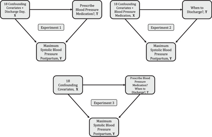 Figure 1
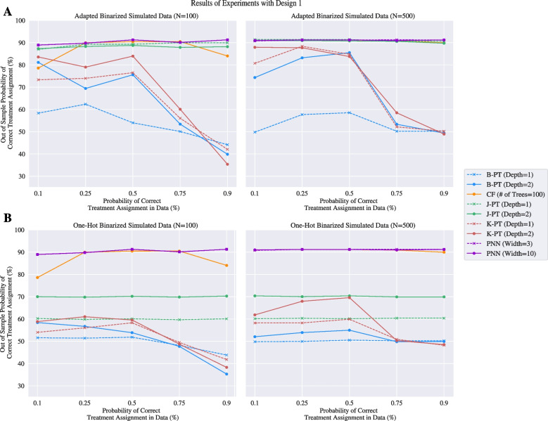 Figure 2
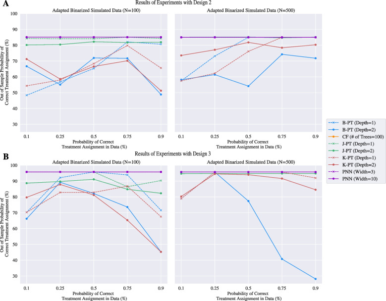 Figure 3
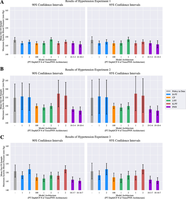 Figure 4
 Figure 5
 Figure 6
 Figure 7
 Figure 8
 Figure 9
- —ObGyn Start-Up–UWF–SMPH Research and Development
Peer Reviews
No public reviews on file for this paper yet. If you reviewed it on a platform where reviews are public (OpenReview, ICLR, NeurIPS, ICML), you can paste yours below so the community can read it here.
Videos
No videos yet. Explain this paper in a talk, walkthrough, or lecture? Add one.
Taxonomy
TopicsMachine Learning in Healthcare · Artificial Intelligence in Healthcare and Education · Explainable Artificial Intelligence (XAI)
Introduction
In high risk domains such as healthcare, getting high quality data can be costly and time consuming to collect. Moreover, the presence of biased or incomplete data can affect quality of care [1, 2]. These challenges are a particular concern in the use of observational data to inform treatment policies. In these problems, the decision maker is interested in using historical data to learn a policy that is capable of mapping patient covariates to treatment options. One example of this is using historical data for hospital readmissions to learn a policy that maps patient chart measures to discharge recommendations. This is a particularly challenging setting, because only observational data can be collected as it is often unethical to obtain a large amount of patient data from randomized controlled trials [3, 4]. In addition to limitations due to ethical concerns, studies involving a small subset of the population, such as treating postpartum birthing persons for hypertension, are naturally data-scarce settings. Moreover, using data that may be biased or incomplete can lead to inaccurate or unreliable models [5]. The consequences of enacting policies derived from such models can include lawsuits, increased costs of insurance, and adverse health effects to individuals targeted by the policy. This can be particularly problematic in public health, where bias in data for a specific demographic leads to discriminatory policies.
To address these challenges, there has been interest in the operations community to develop methods that train prescriptive models, that is, machine learning models that do not just attempt to predict future labels but that also use insights from causal inference to optimize policy treatment effects [6]. Since the key challenge of observational data is that the counterfactual for the treatment is not observed, these methods use techniques such as inverse propensity score weighting [7] or double robust estimation to estimate the treatment effect [8] The resulting models then map patient covariates to the treatment that maximizes this treatment effect. To date, the main models proposed for this task in the literature are decision tree based [6, 9, 10]. The advantage of these models is that they can be optimized effectively using mixed integer programming (MIP) solvers, especially in data scarce settings. However, these models require certain strong assumptions such as requiring binary covariates making their performance contingent on the effectiveness of discretization. Moreover, the resulting decision trees are in general trained to a depth of one or two, meaning that in general only three or so features can be included in the policy computation. While this may be appropriate for some settings, this limits the applicability of these models to settings where treatments depend on multiple patient covariates and their interactions. Thus there is a critical need for developing models that incorporate continuous features and can capture these more complex relationships in the data, while still allowing for exact optimization in this prescriptive setting.
One set of candidate models that could capture this complexity in the data are artificial neural networks (ANNs). In data-rich settings, deep ANNs, i.e, networks with a large number of hidden layers, have taken center stage in learning modern complex tasks. However, current state-of-the-art optimization tools used to train ANNs, such as stochastic gradient descent (SGD), fall short when data availability is limited such as in the prescriptive analytics setting [11–13]. Furthermore, criticisms against the interpretability of deep neural networks are increasingly prevalent in domains such as medicine, public health, and social intervention where fairness and accountability are critical [14–16]. Recent techniques emerging from operations research literature have explored the use of mixed-integer programming to address some of the limitations of ANNs trained with SGD in these data limited settings[17–20]. However, there is currently no consensus on modeling an appropriate loss function for the mixed-integer programming (MIP) formulations. Moreover, the current literature has mainly focused on the training of ANNs for prediction tasks and have not examined their use for prescriptive analytics.
In this paper, we explore the problem of training shallow neural networks with limited data using MIP with a focus on personalized prescription problems. We show that these models have favorable statistical properties, including consistency and asymptotic optimality implying that they can use data efficiently. ANNs trained with SGD may not necessarily have these properties since they may converge to local minima. Furthermore, we provide empirical insight into designing personalized prescription policies in the medical domain where conducting randomized control trials are expensive, unethical, or otherwise infeasible. Specifically, we consider the tasks of deciding treatments for hypertension in postpartum birthing persons. Our methods are well-suited to solve such problems since the availability of data is limited, and the need for understanding which patient characteristics influence policy design is high. In addition to these experiments, in the appendix we provide supplementary experiments showing the use of our prescriptive networks for designing optimal policies to prescribing warfarin for patients susceptible to blood clots. Additionally, in the appendix, we produce empirical results demonstrating the use of our models for prediction using the MNIST digit recognition problem for the 2-digit case.
Problem description
Prescription problems are a growing array of tasks in personalized decision-making. These problems arise when managers and decision-makers need to make general policy decisions that account for the heterogeneous responses to the policy among different individuals in the population. In such cases, prediction alone is not sufficient as individuals may respond to the same treatments differently. These problems are especially challenging to solve in settings with scarce observational data. For instance this occurs in cases where collecting large amounts of controlled data may violate ethical concerns or could be too costly. In settings where data is less scarce or ethical concerns for experimentation are less of a concern, reinforcement learning could be used to learn policies [21–23]. However, these methods are not applicable when these assumptions are violated, necessitating specific techniques for policy learning from observational data. In this paper, we consider the problem of prescribing the best treatment to an individual as a function of their characteristics such that the outcome of such a prescription is optimized.
These problems are particularly challenging because they require us to determine not only what the best treatments are, but also why they are the best treatments. In other words, we need to understand the causal relationships between treatments and outcomes. Indeed, we use techniques from causal inference to define an objective that maximizes (or minimizes) the outcome by estimating the counterfactual information from historical observations. By doing so, we can gain a better understanding of the causal relationships between actions and outcomes, allowing us to make better policy decisions. For instance, when prescribing blood-pressure medication to postpartum patients, we may be interested in ensuring that the model identifies those features that attribute to a positive response to receiving treatment as well as those that attribute to a negative response.
Contributions
The overarching goal of this paper is to provide a structured framework to training ANNs using MIP techniques for prescription problems.
We make several methodological contributions to these problem domains. In the realm of prescription problems, we design an optimization framework that uses MIP-based ANNs, which we refer to as Prescriptive Neural Networks (PNN). PNNs designs interpretable policies with the goal of optimizing population average outcomes given limited observational data. This problem is non-trivial because we need to account for the outcomes of unobserved treatments, as well as incorporate causal effects into our framework. To address this challenge, the PNN optimizes over-estimates of the conditional average treatment effects (CATE) to account for unobserved counterfactual outcomes. To implement the framework into commercial solvers, we propose a novel mixed-integer linear objective function for the prescription problem that incorporates outcomes estimated by the Inverse Propensity Weighting (IPW) method, Direct Method (DM) or the Doubly Robust (DR) estimator. These estimators adjust for confounding factors and provide robust estimates of counterfactual treatment effects using observational data. We also provide statistical guarantees for the proposed formulations that address both prediction and prescription problems. In particular, our analysis shows that these frameworks produce statistically consistent estimators in both cases, to the best of our knowledge this is one of the first derived statistical guarantees for ANNs trained with MIP.
We validated our framework through a series of experiments on both simulated and real-world data. To validate PNNs, we benchmark our methods against state-of-the-art prescriptive methods and heterogeneous treatment effect estimation techniques with simulated experiments common in the prescription literature [24] along with two case studies in personalized healthcare. The first case study entails designing prescriptive policies to treat postpartum patients against hypertension. The second case study, which we present in the appendix, involves incorporating prescription in personalized warfarin dosing. Our contributions also extend to assessing the interpretability of the PNN, and its ability to identify key features that impact in the models’ decisions. By doing so, we derive a sense of our model’s strengths and identify where it is most apt to use prescriptive neural networks over others. In particular, we show that PNNs are more likely to identify relevant clinical features for treatment decisions, unlike existing methods that may use biased surrogate features such as patient insurance information.
While not in the main paper but in the appendix, we also present contribution to the use of MIP ANNs in the realm of prediction. We develop a novel MIP formulation of the negative log-likelihood loss (NLL) that incorporates a softmax activation function applied over the output layer of an ANN formulated by mixed-integer constraints. Existing literature that explores using MIP to train ANNs has considered a Support Vector Machine loss, minimizing empircal classification loss, and other linear and non-linear loss functions [17, 18, 20]. The softmax function is an appealing activation function since it considers the output of the neural network as a probabilistic distribution over predicted output classes [25]. By incorporating this well-studied loss function from the literature into MIP-based ANNs, our work helps bridge the divide between MIP-based training methods and classical training methods. To evaluate the performance of our MIP-based ANN with the NLL objective, we conduct numerical experiments using the MNIST digit recognition dataset. We benchmark our performance against state-of-the-art stochastic gradient descent (SGD) based algorithms. These experiments are conducted over a variety of ANN architectures and hidden-layer activation functions.
Literature review
Our work contributes to several important streams of literature in machine learning and operations research. The MIP formulations we develop in this paper builds upon the existing literature on using integer programming and constraint programming to train ANNs. Our work on applying this framework for personalized prescription problems parallel previous papers that consider the intersection of optimization and statistical inference. In the first stream, we review works that estimate heterogeneous causal effects in the context of learning treatments effects across subsets of the population with causal trees and forests. Along these lines, we also discuss non-tree methods used in statistical learning. Additionally, we present related work on learning prescriptive trees that optimize using MIP formulations. The second stream of literature pertains to training ANNs using MIPs. Finally, we review papers in machine learning that address challenges related to data scarcity and interpretability.
In the context of statistical learning based approaches for causal inference, Athey and Imbens [24] proposed causal tree estimators that use recursive partitions to estimate conditional average treatment effects. The causal tree structure uses the Inverse Propensity Weighting [7] to estimate counterfactual outcomes. Wager and Athey [8] build on the concept of causal trees by extending estimation using random forests with a causal structure, and provide asymptotic confidence intervals for their work. Powers et al. [26] further build on causal forests and introduce Pollinated Transformed Outcome forests for the treatment effect estimation problem in high dimensions. They additionally apply modifications to boosting and MARS (Multivariate Adaptive Regression Splines) to use in the context of structured causal problems. Along the lines of estimating counterfactual estimation, Dudík et al. [27] provides a doubly robust framework that combines inverse propensity weighting methods with “direct methods”, i.e, directly estimating counterfactual outcomes using learning models with a given sample. The same paper proposes methodologies for devising optimal treatment policies using the doubly robust framework. A study on using deep neural networks for semiparametric inference was conducted by Farrell et al. [28], which apply theoretical results on treatment effect and expected welfare estimation.
Several tree-based approaches have been studied in the context of personalized prescription problems. The works reviewed in this avenue of research build on the classification trees [29]. A key motivation presented in literature for personalized trees is to provide a sense of interpretability to prescription problems. Kallus [6] proposes personalization trees with a mixed-integer optimization framework to learn to choose the optimal treatment from a discrete set of treatments. Bertsimas et al. [30] modify this approach with by incorporating regularization for variance-reduction in the objective function of the problem. The authors use coordinate descent with multiple starts to solve the optimization problem numerically. A prescriptive tree approach presented by Jo et al. [10] builds on a MIP-based classification tree [31] formulated as a flow network. One advantage of such a network optimization model is that it is particularly suited for learning in data scarce settings. Both [6] and [30] provide structure for learning optimal trees without explicitly estimating counterfactual outcomes, while the MIP formulation detailed by Jo et al. [10] incorporates inverse propensity weighting methods, direct methods, or doubly robust methods in their optimization problem. Amram et al. [32] extend the work of Bertsimas et al. [30] to the problem of learning prescription policies using estimated counterfactual information, and to problems with continuous-valued treatments. Finally, a new type of prescription trees is presented by Bertsimas et al. [9], which uses threshold-based methods to devise decision-rules that can be used in-tandem with the optimal policy trees [32] under budget constraints.
We now discuss the interplay between integer programming and neural networks in the literature. Using integer programming to train neural networks has gained some popularity in recent years. Toro Icarte et al. [17] use Constraint Programming, MIP, and a hybrid of the two to train Binarized Neural Networks (BNNs), a class of neural networks with the weights and activations restricted to the set {-1, +1}. To relax the binarized restriction on weights, Thorbjarnarson and Yorke-Smith [20] propose a formulation to train Integer Neural Networks with different loss functions. Kurtz and Bah [18] developed a formulation for integer weights, and offer an iterative data splitting algorithm that uses the k-means classification method to train on subsets of data with similar activation patterns. For problems with continuous activation functions, Serra et al. [33] introduce a mixed-integer linear programming (MILP) formulation for deep neural networks to count the number of linear regions represented by it. While the authors do not use the formulation to train neural networks, they utilize a systematic one-tree approach [34] to count integer solutions of the MILP. MIPs have also been used for already trained networks to provide adversarial samples that can improve network stability [35–37]. Additionally, there has been research directed towards using ANNs to solve MIPs [38, 39].
Finally, we discuss additional, non-learning-tree methods that address data scarcity in machine learning and optimization. The promising capabilities of deep learning techniques have spurred compelling research on learning in data scarce settings. Loh [40] proposes a framework that combines supervised and unsupervised learning with prior knowledge of known symmetries or invariance, and surrogate datasets. Hakami [41] suggests the use of Generative Adversarial Networks to generate synthetic data. Additionally, there has been work on utilizing transfer learning techniques that leverage complementary information across different models and datasets [42]. We refer to Alzubaidi et al. [43] for an overview of comprehensive overview of strategies to address data scarcity in training learning models. However, while these techniques show initial promise, it is not clear how applicable they would be to the construction of prescriptive models with observational data, especially in a high stakes setting such as health care. This is because these methods assume that the restricted data sets are fully representative. In contrast, one of the challenges of learning policies from observational data is that only certain patient and treatment combinations are observed, with the counterfactual not being fully represented, making it difficult to generate additional data. Lastly, we highlight some key papers on the importance of interpretability in machine learning applied to healthcare settings [44–47]. These methods show promise in interpreting the predictions of parsimonious models.
Mixed-integer programming formulation of ANNs
In this section we consider MIP formulations for training ANNs in the prescriptive setting. However, in the appendix, we discuss how the formulation can be adapted to the predictive setting, as proposed by Patil and Mintz [19]. Consider a personalized decision-making problem where the goal is to assign the best treatment \documentclass[12pt]{minimal} \usepackage{amsmath} \usepackage{wasysym} \usepackage{amsfonts} \usepackage{amssymb} \usepackage{amsbsy} \usepackage{mathrsfs} \usepackage{upgreek} \setlength{\oddsidemargin}{-69pt} \begin{document}$$t \in \mathcal {T}$$\end{document} for an individual given their covariates \documentclass[12pt]{minimal} \usepackage{amsmath} \usepackage{wasysym} \usepackage{amsfonts} \usepackage{amssymb} \usepackage{amsbsy} \usepackage{mathrsfs} \usepackage{upgreek} \setlength{\oddsidemargin}{-69pt} \begin{document}$$X \in \mathcal {X} \subseteq \mathbb {R}^\mathcal {F}$$\end{document} such that the individual’s potential outcome \documentclass[12pt]{minimal} \usepackage{amsmath} \usepackage{wasysym} \usepackage{amsfonts} \usepackage{amssymb} \usepackage{amsbsy} \usepackage{mathrsfs} \usepackage{upgreek} \setlength{\oddsidemargin}{-69pt} \begin{document}$$Y(t) \in \mathcal {Y} \subseteq \mathbb {R}$$\end{document} is either minimized or maximized over the treatment group. We assume both \documentclass[12pt]{minimal} \usepackage{amsmath} \usepackage{wasysym} \usepackage{amsfonts} \usepackage{amssymb} \usepackage{amsbsy} \usepackage{mathrsfs} \usepackage{upgreek} \setlength{\oddsidemargin}{-69pt} \begin{document}$$\mathcal {X},\mathcal {Y}$$\end{document} are compact sets and that \documentclass[12pt]{minimal} \usepackage{amsmath} \usepackage{wasysym} \usepackage{amsfonts} \usepackage{amssymb} \usepackage{amsbsy} \usepackage{mathrsfs} \usepackage{upgreek} \setlength{\oddsidemargin}{-69pt} \begin{document}$$\mathcal {T}$$\end{document} is a finite set. In this problem, decision-makers use observational data to design a personalized treatment policy \documentclass[12pt]{minimal} \usepackage{amsmath} \usepackage{wasysym} \usepackage{amsfonts} \usepackage{amssymb} \usepackage{amsbsy} \usepackage{mathrsfs} \usepackage{upgreek} \setlength{\oddsidemargin}{-69pt} \begin{document}$$s: \mathcal {X} \mapsto \mathcal {T}$$\end{document} that should then be able to prescribe an optimal treatment s(X) for an individual based on their covariates X. In the case where all of the potential outcomes \documentclass[12pt]{minimal} \usepackage{amsmath} \usepackage{wasysym} \usepackage{amsfonts} \usepackage{amssymb} \usepackage{amsbsy} \usepackage{mathrsfs} \usepackage{upgreek} \setlength{\oddsidemargin}{-69pt} \begin{document}$$\{Y_i(t)\}_{t\in \mathcal {T}}$$\end{document} for an individual i are known, the problem of learning an optimal policy \documentclass[12pt]{minimal} \usepackage{amsmath} \usepackage{wasysym} \usepackage{amsfonts} \usepackage{amssymb} \usepackage{amsbsy} \usepackage{mathrsfs} \usepackage{upgreek} \setlength{\oddsidemargin}{-69pt} \begin{document}$$\hat{s}$$\end{document} is a classification problem where the model classifies the patient to the treatment group that maximizes or minimizes individual’s outcome. Recall that we are interested in the observational case when prescribing a patient every possible treatment to procure all potential outcomes can be impractical due to ethical concerns or resource constraints. In this problem, we observe an outcome \documentclass[12pt]{minimal} \usepackage{amsmath} \usepackage{wasysym} \usepackage{amsfonts} \usepackage{amssymb} \usepackage{amsbsy} \usepackage{mathrsfs} \usepackage{upgreek} \setlength{\oddsidemargin}{-69pt} \begin{document}$$\{Y_i(t_i)\}$$\end{document} for individual \documentclass[12pt]{minimal} \usepackage{amsmath} \usepackage{wasysym} \usepackage{amsfonts} \usepackage{amssymb} \usepackage{amsbsy} \usepackage{mathrsfs} \usepackage{upgreek} \setlength{\oddsidemargin}{-69pt} \begin{document}$$i \in \{1,\ldots ,n\}$$\end{document} having received treatment \documentclass[12pt]{minimal} \usepackage{amsmath} \usepackage{wasysym} \usepackage{amsfonts} \usepackage{amssymb} \usepackage{amsbsy} \usepackage{mathrsfs} \usepackage{upgreek} \setlength{\oddsidemargin}{-69pt} \begin{document}$$t_i$$\end{document} , but not their counterfactual outcomes \documentclass[12pt]{minimal} \usepackage{amsmath} \usepackage{wasysym} \usepackage{amsfonts} \usepackage{amssymb} \usepackage{amsbsy} \usepackage{mathrsfs} \usepackage{upgreek} \setlength{\oddsidemargin}{-69pt} \begin{document}$$\{Y_i(t)\}_{t \in \mathcal {T} \setminus t_i}$$\end{document} . Our goal is to learn a policy \documentclass[12pt]{minimal} \usepackage{amsmath} \usepackage{wasysym} \usepackage{amsfonts} \usepackage{amssymb} \usepackage{amsbsy} \usepackage{mathrsfs} \usepackage{upgreek} \setlength{\oddsidemargin}{-69pt} \begin{document}$$\hat{s}$$\end{document} from n independent and identically distributed observations of participants \documentclass[12pt]{minimal} \usepackage{amsmath} \usepackage{wasysym} \usepackage{amsfonts} \usepackage{amssymb} \usepackage{amsbsy} \usepackage{mathrsfs} \usepackage{upgreek} \setlength{\oddsidemargin}{-69pt} \begin{document}$$\{(X_1, t_1, Y_1(t_1)), \ldots , (X_n, t_n, Y_n(t_n))\}$$\end{document} .
We use the notation \documentclass[12pt]{minimal} \usepackage{amsmath} \usepackage{wasysym} \usepackage{amsfonts} \usepackage{amssymb} \usepackage{amsbsy} \usepackage{mathrsfs} \usepackage{upgreek} \setlength{\oddsidemargin}{-69pt} \begin{document}$$[n]_m = \{m,m+1,...,n\}$$\end{document} for any two integers \documentclass[12pt]{minimal} \usepackage{amsmath} \usepackage{wasysym} \usepackage{amsfonts} \usepackage{amssymb} \usepackage{amsbsy} \usepackage{mathrsfs} \usepackage{upgreek} \setlength{\oddsidemargin}{-69pt} \begin{document}$$n>m$$\end{document} . For our problem, we will think of policies s being parameterized by \documentclass[12pt]{minimal} \usepackage{amsmath} \usepackage{wasysym} \usepackage{amsfonts} \usepackage{amssymb} \usepackage{amsbsy} \usepackage{mathrsfs} \usepackage{upgreek} \setlength{\oddsidemargin}{-69pt} \begin{document}$$\theta \in \Theta$$\end{document} , where \documentclass[12pt]{minimal} \usepackage{amsmath} \usepackage{wasysym} \usepackage{amsfonts} \usepackage{amssymb} \usepackage{amsbsy} \usepackage{mathrsfs} \usepackage{upgreek} \setlength{\oddsidemargin}{-69pt} \begin{document}$$\Theta$$\end{document} is a compact set, and our goal will be to find \documentclass[12pt]{minimal} \usepackage{amsmath} \usepackage{wasysym} \usepackage{amsfonts} \usepackage{amssymb} \usepackage{amsbsy} \usepackage{mathrsfs} \usepackage{upgreek} \setlength{\oddsidemargin}{-69pt} \begin{document}$$\theta ^*$$\end{document} such that for any \documentclass[12pt]{minimal} \usepackage{amsmath} \usepackage{wasysym} \usepackage{amsfonts} \usepackage{amssymb} \usepackage{amsbsy} \usepackage{mathrsfs} \usepackage{upgreek} \setlength{\oddsidemargin}{-69pt} \begin{document}$$X\in \mathcal {X}$$\end{document} , \documentclass[12pt]{minimal} \usepackage{amsmath} \usepackage{wasysym} \usepackage{amsfonts} \usepackage{amssymb} \usepackage{amsbsy} \usepackage{mathrsfs} \usepackage{upgreek} \setlength{\oddsidemargin}{-69pt} \begin{document}$$s(X;\theta ^*)$$\end{document} is able to closely predict the optimal treatment. Our goal will be to estimate \documentclass[12pt]{minimal} \usepackage{amsmath} \usepackage{wasysym} \usepackage{amsfonts} \usepackage{amssymb} \usepackage{amsbsy} \usepackage{mathrsfs} \usepackage{upgreek} \setlength{\oddsidemargin}{-69pt} \begin{document}$$\theta ^*$$\end{document} by finding a \documentclass[12pt]{minimal} \usepackage{amsmath} \usepackage{wasysym} \usepackage{amsfonts} \usepackage{amssymb} \usepackage{amsbsy} \usepackage{mathrsfs} \usepackage{upgreek} \setlength{\oddsidemargin}{-69pt} \begin{document}$$\hat{\theta }$$\end{document} that minimizes an empirical loss \documentclass[12pt]{minimal} \usepackage{amsmath} \usepackage{wasysym} \usepackage{amsfonts} \usepackage{amssymb} \usepackage{amsbsy} \usepackage{mathrsfs} \usepackage{upgreek} \setlength{\oddsidemargin}{-69pt} \begin{document}$$\mathcal {L}_n: \mathcal {T}\times \mathcal {Y} \mapsto \mathbb {R}$$\end{document} that is \documentclass[12pt]{minimal} \usepackage{amsmath} \usepackage{wasysym} \usepackage{amsfonts} \usepackage{amssymb} \usepackage{amsbsy} \usepackage{mathrsfs} \usepackage{upgreek} \setlength{\oddsidemargin}{-69pt} \begin{document}$$\hat{\theta } = \textrm{argmin}_{\theta \in \Theta } \frac{1}{n}\sum _{i = 1}^n \mathcal {L}_n(s(X_i;\theta ),Y_i)$$\end{document} . We assume s is an ANN that can be expressed as a functional composition of L vector valued functions that is \documentclass[12pt]{minimal} \usepackage{amsmath} \usepackage{wasysym} \usepackage{amsfonts} \usepackage{amssymb} \usepackage{amsbsy} \usepackage{mathrsfs} \usepackage{upgreek} \setlength{\oddsidemargin}{-69pt} \begin{document}$$s(X;\theta ) = h_L\circ h_{L-1} \circ ... \circ h_1 \circ h_0(x)$$\end{document} . Here each function \documentclass[12pt]{minimal} \usepackage{amsmath} \usepackage{wasysym} \usepackage{amsfonts} \usepackage{amssymb} \usepackage{amsbsy} \usepackage{mathrsfs} \usepackage{upgreek} \setlength{\oddsidemargin}{-69pt} \begin{document}$$h_\ell (\cdot ,\theta _\ell )$$\end{document} is referred to as a layer of the neural network, we assume that \documentclass[12pt]{minimal} \usepackage{amsmath} \usepackage{wasysym} \usepackage{amsfonts} \usepackage{amssymb} \usepackage{amsbsy} \usepackage{mathrsfs} \usepackage{upgreek} \setlength{\oddsidemargin}{-69pt} \begin{document}$$h_0:\mathcal{X} \mapsto \mathbb{R}^K$$\end{document} , \documentclass[12pt]{minimal} \usepackage{amsmath} \usepackage{wasysym} \usepackage{amsfonts} \usepackage{amssymb} \usepackage{amsbsy} \usepackage{mathrsfs} \usepackage{upgreek} \setlength{\oddsidemargin}{-69pt} \begin{document}$$h_L:\mathbb {R}^K \mapsto \mathcal {T}$$\end{document} , and \documentclass[12pt]{minimal} \usepackage{amsmath} \usepackage{wasysym} \usepackage{amsfonts} \usepackage{amssymb} \usepackage{amsbsy} \usepackage{mathrsfs} \usepackage{upgreek} \setlength{\oddsidemargin}{-69pt} \begin{document}$$h_\ell : \mathbb {R}^K \mapsto \mathbb {R}^K$$\end{document} , we denote each component of \documentclass[12pt]{minimal} \usepackage{amsmath} \usepackage{wasysym} \usepackage{amsfonts} \usepackage{amssymb} \usepackage{amsbsy} \usepackage{mathrsfs} \usepackage{upgreek} \setlength{\oddsidemargin}{-69pt} \begin{document}$$h_\ell$$\end{document} as \documentclass[12pt]{minimal} \usepackage{amsmath} \usepackage{wasysym} \usepackage{amsfonts} \usepackage{amssymb} \usepackage{amsbsy} \usepackage{mathrsfs} \usepackage{upgreek} \setlength{\oddsidemargin}{-69pt} \begin{document}$$h_{k,\ell }$$\end{document} for \documentclass[12pt]{minimal} \usepackage{amsmath} \usepackage{wasysym} \usepackage{amsfonts} \usepackage{amssymb} \usepackage{amsbsy} \usepackage{mathrsfs} \usepackage{upgreek} \setlength{\oddsidemargin}{-69pt} \begin{document}$$\ell \in [L-1]_0$$\end{document} and \documentclass[12pt]{minimal} \usepackage{amsmath} \usepackage{wasysym} \usepackage{amsfonts} \usepackage{amssymb} \usepackage{amsbsy} \usepackage{mathrsfs} \usepackage{upgreek} \setlength{\oddsidemargin}{-69pt} \begin{document}$$k \in [K]_1$$\end{document} , and each component of \documentclass[12pt]{minimal} \usepackage{amsmath} \usepackage{wasysym} \usepackage{amsfonts} \usepackage{amssymb} \usepackage{amsbsy} \usepackage{mathrsfs} \usepackage{upgreek} \setlength{\oddsidemargin}{-69pt} \begin{document}$$h_L$$\end{document} as \documentclass[12pt]{minimal} \usepackage{amsmath} \usepackage{wasysym} \usepackage{amsfonts} \usepackage{amssymb} \usepackage{amsbsy} \usepackage{mathrsfs} \usepackage{upgreek} \setlength{\oddsidemargin}{-69pt} \begin{document}$$h_{t,L}$$\end{document} for \documentclass[12pt]{minimal} \usepackage{amsmath} \usepackage{wasysym} \usepackage{amsfonts} \usepackage{amssymb} \usepackage{amsbsy} \usepackage{mathrsfs} \usepackage{upgreek} \setlength{\oddsidemargin}{-69pt} \begin{document}$$t \in \mathcal {T}$$\end{document} . We refer to these components as units or neurons. We refer to the index \documentclass[12pt]{minimal} \usepackage{amsmath} \usepackage{wasysym} \usepackage{amsfonts} \usepackage{amssymb} \usepackage{amsbsy} \usepackage{mathrsfs} \usepackage{upgreek} \setlength{\oddsidemargin}{-69pt} \begin{document}$$\ell$$\end{document} as the layer number of the ANN, and the index k as the unit number. The layer corresponding to the index L is referred to as the output layer, and all other indices are referred to as hidden layers. Each unit has the functional form: \documentclass[12pt]{minimal} \usepackage{amsmath} \usepackage{wasysym} \usepackage{amsfonts} \usepackage{amssymb} \usepackage{amsbsy} \usepackage{mathrsfs} \usepackage{upgreek} \setlength{\oddsidemargin}{-69pt} \begin{document}$$h_{k,0} = \sigma (\alpha _{k,0}^\top X + \beta _{k,0})$$\end{document} , \documentclass[12pt]{minimal} \usepackage{amsmath} \usepackage{wasysym} \usepackage{amsfonts} \usepackage{amssymb} \usepackage{amsbsy} \usepackage{mathrsfs} \usepackage{upgreek} \setlength{\oddsidemargin}{-69pt} \begin{document}$$h_{k,\ell } = \sigma (\alpha _{k,\ell }^\top h_{\ell -1} + \beta _{k,\ell })$$\end{document} for \documentclass[12pt]{minimal} \usepackage{amsmath} \usepackage{wasysym} \usepackage{amsfonts} \usepackage{amssymb} \usepackage{amsbsy} \usepackage{mathrsfs} \usepackage{upgreek} \setlength{\oddsidemargin}{-69pt} \begin{document}$$\ell \in [L-1]_1$$\end{document} , \documentclass[12pt]{minimal} \usepackage{amsmath} \usepackage{wasysym} \usepackage{amsfonts} \usepackage{amssymb} \usepackage{amsbsy} \usepackage{mathrsfs} \usepackage{upgreek} \setlength{\oddsidemargin}{-69pt} \begin{document}$$h_{t,L} = \varphi (\alpha _{t,L}^\top h_{L-1} + \beta _{t,L})$$\end{document} , where \documentclass[12pt]{minimal} \usepackage{amsmath} \usepackage{wasysym} \usepackage{amsfonts} \usepackage{amssymb} \usepackage{amsbsy} \usepackage{mathrsfs} \usepackage{upgreek} \setlength{\oddsidemargin}{-69pt} \begin{document}$$\sigma :\mathbb {R}\mapsto \mathbb {R}$$\end{document} is a non-linear function applied over the hidden layers \documentclass[12pt]{minimal} \usepackage{amsmath} \usepackage{wasysym} \usepackage{amsfonts} \usepackage{amssymb} \usepackage{amsbsy} \usepackage{mathrsfs} \usepackage{upgreek} \setlength{\oddsidemargin}{-69pt} \begin{document}$$\ell = 0,...,L-1$$\end{document} called the activation function, \documentclass[12pt]{minimal} \usepackage{amsmath} \usepackage{wasysym} \usepackage{amsfonts} \usepackage{amssymb} \usepackage{amsbsy} \usepackage{mathrsfs} \usepackage{upgreek} \setlength{\oddsidemargin}{-69pt} \begin{document}$$\varphi :\mathbb {R}\mapsto \mathbb {R}$$\end{document} is a potentially different non-linear function applied over the output layer L, and \documentclass[12pt]{minimal} \usepackage{amsmath} \usepackage{wasysym} \usepackage{amsfonts} \usepackage{amssymb} \usepackage{amsbsy} \usepackage{mathrsfs} \usepackage{upgreek} \setlength{\oddsidemargin}{-69pt} \begin{document}$$\alpha$$\end{document} and \documentclass[12pt]{minimal} \usepackage{amsmath} \usepackage{wasysym} \usepackage{amsfonts} \usepackage{amssymb} \usepackage{amsbsy} \usepackage{mathrsfs} \usepackage{upgreek} \setlength{\oddsidemargin}{-69pt} \begin{document}$$\beta$$\end{document} are the weights and biases matrices respectively where \documentclass[12pt]{minimal} \usepackage{amsmath} \usepackage{wasysym} \usepackage{amsfonts} \usepackage{amssymb} \usepackage{amsbsy} \usepackage{mathrsfs} \usepackage{upgreek} \setlength{\oddsidemargin}{-69pt} \begin{document}$$(\alpha ,\beta ) = \theta$$\end{document} . In our work, we consider \documentclass[12pt]{minimal} \usepackage{amsmath} \usepackage{wasysym} \usepackage{amsfonts} \usepackage{amssymb} \usepackage{amsbsy} \usepackage{mathrsfs} \usepackage{upgreek} \setlength{\oddsidemargin}{-69pt} \begin{document}$$\sigma$$\end{document} to be the binary activation and we assume for any input \documentclass[12pt]{minimal} \usepackage{amsmath} \usepackage{wasysym} \usepackage{amsfonts} \usepackage{amssymb} \usepackage{amsbsy} \usepackage{mathrsfs} \usepackage{upgreek} \setlength{\oddsidemargin}{-69pt} \begin{document}$$z \in \mathbb {R}$$\end{document} , \documentclass[12pt]{minimal} \usepackage{amsmath} \usepackage{wasysym} \usepackage{amsfonts} \usepackage{amssymb} \usepackage{amsbsy} \usepackage{mathrsfs} \usepackage{upgreek} \setlength{\oddsidemargin}{-69pt} \begin{document}$$\sigma (z) = \mathbf{1}[z \ge 0]$$\end{document} , where \documentclass[12pt]{minimal} \usepackage{amsmath} \usepackage{wasysym} \usepackage{amsfonts} \usepackage{amssymb} \usepackage{amsbsy} \usepackage{mathrsfs} \usepackage{upgreek} \setlength{\oddsidemargin}{-69pt} \begin{document}$$\mathbf {1}$$\end{document} is the indicator function. The notation \documentclass[12pt]{minimal} \usepackage{amsmath} \usepackage{wasysym} \usepackage{amsfonts} \usepackage{amssymb} \usepackage{amsbsy} \usepackage{mathrsfs} \usepackage{upgreek} \setlength{\oddsidemargin}{-69pt} \begin{document}$$\alpha _{a,b,\ell }$$\end{document} indicates the weight being applied to unit index a in layer \documentclass[12pt]{minimal} \usepackage{amsmath} \usepackage{wasysym} \usepackage{amsfonts} \usepackage{amssymb} \usepackage{amsbsy} \usepackage{mathrsfs} \usepackage{upgreek} \setlength{\oddsidemargin}{-69pt} \begin{document}$$\ell -1$$\end{document} for the evaluation of unit index b in layer \documentclass[12pt]{minimal} \usepackage{amsmath} \usepackage{wasysym} \usepackage{amsfonts} \usepackage{amssymb} \usepackage{amsbsy} \usepackage{mathrsfs} \usepackage{upgreek} \setlength{\oddsidemargin}{-69pt} \begin{document}$$\ell$$\end{document} . Likewise, \documentclass[12pt]{minimal} \usepackage{amsmath} \usepackage{wasysym} \usepackage{amsfonts} \usepackage{amssymb} \usepackage{amsbsy} \usepackage{mathrsfs} \usepackage{upgreek} \setlength{\oddsidemargin}{-69pt} \begin{document}$$\beta _{k,\ell }$$\end{document} indicates the bias associated with unit index k in layer \documentclass[12pt]{minimal} \usepackage{amsmath} \usepackage{wasysym} \usepackage{amsfonts} \usepackage{amssymb} \usepackage{amsbsy} \usepackage{mathrsfs} \usepackage{upgreek} \setlength{\oddsidemargin}{-69pt} \begin{document}$$\ell$$\end{document} of the network.
We show how the above training problem and model can be formulated as a MIP. The key to our reformulation is the introduction of decision variables \documentclass[12pt]{minimal} \usepackage{amsmath} \usepackage{wasysym} \usepackage{amsfonts} \usepackage{amssymb} \usepackage{amsbsy} \usepackage{mathrsfs} \usepackage{upgreek} \setlength{\oddsidemargin}{-69pt} \begin{document}$$h_{i,k,\ell }$$\end{document} which correspond to the unit output of unit k in layer \documentclass[12pt]{minimal} \usepackage{amsmath} \usepackage{wasysym} \usepackage{amsfonts} \usepackage{amssymb} \usepackage{amsbsy} \usepackage{mathrsfs} \usepackage{upgreek} \setlength{\oddsidemargin}{-69pt} \begin{document}$$\ell$$\end{document} when the ANN is evaluated at data point with index i. Having these decision variables be data point dependant, and ensuring that \documentclass[12pt]{minimal} \usepackage{amsmath} \usepackage{wasysym} \usepackage{amsfonts} \usepackage{amssymb} \usepackage{amsbsy} \usepackage{mathrsfs} \usepackage{upgreek} \setlength{\oddsidemargin}{-69pt} \begin{document}$$\alpha _{k^\prime ,k,\ell },\beta _{k,\ell }$$\end{document} are the same across all data points forms the backbone of our formulation. Thus, if \documentclass[12pt]{minimal} \usepackage{amsmath} \usepackage{wasysym} \usepackage{amsfonts} \usepackage{amssymb} \usepackage{amsbsy} \usepackage{mathrsfs} \usepackage{upgreek} \setlength{\oddsidemargin}{-69pt} \begin{document}$$X_{i,d}$$\end{document} denotes the \documentclass[12pt]{minimal} \usepackage{amsmath} \usepackage{wasysym} \usepackage{amsfonts} \usepackage{amssymb} \usepackage{amsbsy} \usepackage{mathrsfs} \usepackage{upgreek} \setlength{\oddsidemargin}{-69pt} \begin{document}$$d^{th}$$\end{document} feature value of individual i, the general form of the optimization problem is:
\documentclass[12pt]{minimal} \usepackage{amsmath} \usepackage{wasysym} \usepackage{amsfonts} \usepackage{amssymb} \usepackage{amsbsy} \usepackage{mathrsfs} \usepackage{upgreek} \setlength{\oddsidemargin}{-69pt} \begin{document}$$\begin{aligned} \hat{\theta }_n = \mathop {\mathrm {arg\,min}}\limits _{\theta \in \Theta }&\frac{1}{n}\sum _{i=1}^n\sum _{t \in T} \mathcal {L}_n(h_{i,t,L},y_{i,j})&\end{aligned}$$\end{document} \documentclass[12pt]{minimal} \usepackage{amsmath} \usepackage{wasysym} \usepackage{amsfonts} \usepackage{amssymb} \usepackage{amsbsy} \usepackage{mathrsfs} \usepackage{upgreek} \setlength{\oddsidemargin}{-69pt} \begin{document}$$\begin{aligned} \text {subject to } \nonumber \\&h_{i,k,0} = \sigma (\sum _{d \in \mathcal {F}}\alpha _{d,k,0}X_{i,d} + \beta _{k,0}), \nonumber \\ &\forall \ k,i \in [K]_1 \times [n]_1, \end{aligned}$$\end{document} \documentclass[12pt]{minimal} \usepackage{amsmath} \usepackage{wasysym} \usepackage{amsfonts} \usepackage{amssymb} \usepackage{amsbsy} \usepackage{mathrsfs} \usepackage{upgreek} \setlength{\oddsidemargin}{-69pt} \begin{document}$$\begin{aligned}&h_{i,k,\ell } = \sigma (\sum _{k'=1}^K\alpha _{k^\prime ,k,\ell }h_{i,k^\prime ,\ell -1} + \beta _{k,\ell }), \nonumber \\ &\forall \ \ell ,k,i \in [L-1]_1 \times [K]_1 \times [n]_1, \end{aligned}$$\end{document} \documentclass[12pt]{minimal} \usepackage{amsmath} \usepackage{wasysym} \usepackage{amsfonts} \usepackage{amssymb} \usepackage{amsbsy} \usepackage{mathrsfs} \usepackage{upgreek} \setlength{\oddsidemargin}{-69pt} \begin{document}$$\begin{aligned}&h_{i,t,L} = \varphi (\sum _{k'=1}^K\alpha _{k^\prime ,j,L}h_{i,k^\prime ,L-1} + \beta _{t,L}), \nonumber \\ &\forall j,i \in \mathcal {T} \times [n]_1. \end{aligned}$$\end{document}In this section we will discuss how the constraints of (1) can be represented using a MIP formulation. We will also discuss how different forms of common causal inference loss functions \documentclass[12pt]{minimal} \usepackage{amsmath} \usepackage{wasysym} \usepackage{amsfonts} \usepackage{amssymb} \usepackage{amsbsy} \usepackage{mathrsfs} \usepackage{upgreek} \setlength{\oddsidemargin}{-69pt} \begin{document}$$\mathcal {L}_n$$\end{document} can be formulated using MIP constraints. We will conclude by proving that the resulting formulation provides consistent estimates of the optimal policy. That is, that as \documentclass[12pt]{minimal} \usepackage{amsmath} \usepackage{wasysym} \usepackage{amsfonts} \usepackage{amssymb} \usepackage{amsbsy} \usepackage{mathrsfs} \usepackage{upgreek} \setlength{\oddsidemargin}{-69pt} \begin{document}$$n \rightarrow \infty$$\end{document} , \documentclass[12pt]{minimal} \usepackage{amsmath} \usepackage{wasysym} \usepackage{amsfonts} \usepackage{amssymb} \usepackage{amsbsy} \usepackage{mathrsfs} \usepackage{upgreek} \setlength{\oddsidemargin}{-69pt} \begin{document}$$\hat{\theta }_n \overset{p}{\rightarrow }\ \theta ^*$$\end{document} . This property is crucial, since it indicates that as decision makers gather more data our technique will generate more effective policies. Moreover, it is not clear if many ANN architectures trained using stochastic gradient based approaches exhibit this property in general.
Binary activations
In this section, we present a MIP reformulation of the constraints of (1) for binary activations in the hidden layers that can be solved using commercial solvers. Our formulation can be seen as an extension of prior MIP formulations for ANN training by using continuous instead of integer valued model weights [17]. Specifically, we relax the bounds such that \documentclass[12pt]{minimal} \usepackage{amsmath} \usepackage{wasysym} \usepackage{amsfonts} \usepackage{amssymb} \usepackage{amsbsy} \usepackage{mathrsfs} \usepackage{upgreek} \setlength{\oddsidemargin}{-69pt} \begin{document}$$\alpha _{d,k,0}, \alpha _{k^\prime ,k,l},$$\end{document} \documentclass[12pt]{minimal} \usepackage{amsmath} \usepackage{wasysym} \usepackage{amsfonts} \usepackage{amssymb} \usepackage{amsbsy} \usepackage{mathrsfs} \usepackage{upgreek} \setlength{\oddsidemargin}{-69pt} \begin{document}$$\alpha _{k^\prime ,j,L} \in [\alpha ^{L}, \alpha ^{U}]$$\end{document} . We rewrite Constraints (2),(3),(4) for a single unit as \documentclass[12pt]{minimal} \usepackage{amsmath} \usepackage{wasysym} \usepackage{amsfonts} \usepackage{amssymb} \usepackage{amsbsy} \usepackage{mathrsfs} \usepackage{upgreek} \setlength{\oddsidemargin}{-69pt} \begin{document}$$h_{i,k,0} = \mathbb {1}$$\end{document} \documentclass[12pt]{minimal} \usepackage{amsmath} \usepackage{wasysym} \usepackage{amsfonts} \usepackage{amssymb} \usepackage{amsbsy} \usepackage{mathrsfs} \usepackage{upgreek} \setlength{\oddsidemargin}{-69pt} \begin{document}$$[ \sum _{d \in \mathcal {F}} \alpha _{d,k,0}$$\end{document} \documentclass[12pt]{minimal} \usepackage{amsmath} \usepackage{wasysym} \usepackage{amsfonts} \usepackage{amssymb} \usepackage{amsbsy} \usepackage{mathrsfs} \usepackage{upgreek} \setlength{\oddsidemargin}{-69pt} \begin{document}$$X_{i,d} + \beta _{k,X0} \ge 0]$$\end{document} , \documentclass[12pt]{minimal} \usepackage{amsmath} \usepackage{wasysym} \usepackage{amsfonts} \usepackage{amssymb} \usepackage{amsbsy} \usepackage{mathrsfs} \usepackage{upgreek} \setlength{\oddsidemargin}{-69pt} \begin{document}$$h_{i,k,\ell } = \mathbf {1}[ \sum _{k^\prime =1}^K$$\end{document} \documentclass[12pt]{minimal} \usepackage{amsmath} \usepackage{wasysym} \usepackage{amsfonts} \usepackage{amssymb} \usepackage{amsbsy} \usepackage{mathrsfs} \usepackage{upgreek} \setlength{\oddsidemargin}{-69pt} \begin{document}$$\alpha _{k,k^\prime ,\ell }$$\end{document} \documentclass[12pt]{minimal} \usepackage{amsmath} \usepackage{wasysym} \usepackage{amsfonts} \usepackage{amssymb} \usepackage{amsbsy} \usepackage{mathrsfs} \usepackage{upgreek} \setlength{\oddsidemargin}{-69pt} \begin{document}$$h_{i,k^\prime ,\ell -1} +$$\end{document} \documentclass[12pt]{minimal} \usepackage{amsmath} \usepackage{wasysym} \usepackage{amsfonts} \usepackage{amssymb} \usepackage{amsbsy} \usepackage{mathrsfs} \usepackage{upgreek} \setlength{\oddsidemargin}{-69pt} \begin{document}$$\beta _{k,\ell } \ge 0]$$\end{document} , \documentclass[12pt]{minimal} \usepackage{amsmath} \usepackage{wasysym} \usepackage{amsfonts} \usepackage{amssymb} \usepackage{amsbsy} \usepackage{mathrsfs} \usepackage{upgreek} \setlength{\oddsidemargin}{-69pt} \begin{document}$$h_{i,j,L} =$$\end{document} \documentclass[12pt]{minimal} \usepackage{amsmath} \usepackage{wasysym} \usepackage{amsfonts} \usepackage{amssymb} \usepackage{amsbsy} \usepackage{mathrsfs} \usepackage{upgreek} \setlength{\oddsidemargin}{-69pt} \begin{document}$$\sum _{k^\prime =1}^K \alpha _{k^\prime ,j,L}$$\end{document} \documentclass[12pt]{minimal} \usepackage{amsmath} \usepackage{wasysym} \usepackage{amsfonts} \usepackage{amssymb} \usepackage{amsbsy} \usepackage{mathrsfs} \usepackage{upgreek} \setlength{\oddsidemargin}{-69pt} \begin{document}$$h_{i,k^\prime ,L-1} + \beta _{j,\ell }$$\end{document} respectively. Note that for all layers that are not the input layer, the above constraints contain bi-linear products which make this formulation challenging to solve. We propose the following reformulation:
Proposition 1
In the binary activation case, the Constraints (2),(3),(4) can be reformulated as a set of MIP constraints. Specifically for all \documentclass[12pt]{minimal} \usepackage{amsmath} \usepackage{wasysym} \usepackage{amsfonts} \usepackage{amssymb} \usepackage{amsbsy} \usepackage{mathrsfs} \usepackage{upgreek} \setlength{\oddsidemargin}{-69pt} \begin{document}$$k\in [K]_1, i\in [n]_1$$\end{document} Constraint (2) can be reformulated as:
\documentclass[12pt]{minimal} \usepackage{amsmath} \usepackage{wasysym} \usepackage{amsfonts} \usepackage{amssymb} \usepackage{amsbsy} \usepackage{mathrsfs} \usepackage{upgreek} \setlength{\oddsidemargin}{-69pt} \begin{document}$$\begin{aligned}&\sum _{d \in \mathcal {F}} (\alpha _{d,k,0}X_{i,d}) + \beta _{k,0} \le Mh_{i,k,0}, \end{aligned}$$\end{document} \documentclass[12pt]{minimal} \usepackage{amsmath} \usepackage{wasysym} \usepackage{amsfonts} \usepackage{amssymb} \usepackage{amsbsy} \usepackage{mathrsfs} \usepackage{upgreek} \setlength{\oddsidemargin}{-69pt} \begin{document}$$\begin{aligned}&\sum _{d \in \mathcal {F}} (\alpha _{d,k,0}X_{i,d}) + \beta _{k,0} \ge \epsilon + (-M-\epsilon )(1-h_{i,k,0}), \end{aligned}$$\end{document}For all, \documentclass[12pt]{minimal} \usepackage{amsmath} \usepackage{wasysym} \usepackage{amsfonts} \usepackage{amssymb} \usepackage{amsbsy} \usepackage{mathrsfs} \usepackage{upgreek} \setlength{\oddsidemargin}{-69pt} \begin{document}$$\ell \in [L-1]_1,k\in [K]_1,i\in [n]_1$$\end{document} Constraints (3) can be reformulated as:
\documentclass[12pt]{minimal} \usepackage{amsmath} \usepackage{wasysym} \usepackage{amsfonts} \usepackage{amssymb} \usepackage{amsbsy} \usepackage{mathrsfs} \usepackage{upgreek} \setlength{\oddsidemargin}{-69pt} \begin{document}$$\begin{aligned}&\sum _{k^\prime =1}^{K} (z_{i,k^\prime ,k,\ell }) + \beta _{k,\ell } \le Mh_{i,k,\ell }, \end{aligned}$$\end{document} \documentclass[12pt]{minimal} \usepackage{amsmath} \usepackage{wasysym} \usepackage{amsfonts} \usepackage{amssymb} \usepackage{amsbsy} \usepackage{mathrsfs} \usepackage{upgreek} \setlength{\oddsidemargin}{-69pt} \begin{document}$$\begin{aligned}&\sum _{k^\prime =1}^{K} (z_{i,k^\prime ,k,\ell }) + \beta _{k,\ell } \ge \epsilon + (-M-\epsilon )(1-h_{i,k,\ell }), \end{aligned}$$\end{document} \documentclass[12pt]{minimal} \usepackage{amsmath} \usepackage{wasysym} \usepackage{amsfonts} \usepackage{amssymb} \usepackage{amsbsy} \usepackage{mathrsfs} \usepackage{upgreek} \setlength{\oddsidemargin}{-69pt} \begin{document}$$\begin{aligned}&z_{i,k^\prime ,k,\ell } \le \alpha _{k^\prime ,k,\ell } + M(1-h_{i,k^\prime ,\ell -1}), \ \forall \ k^\prime \in [K]_1, \end{aligned}$$\end{document} \documentclass[12pt]{minimal} \usepackage{amsmath} \usepackage{wasysym} \usepackage{amsfonts} \usepackage{amssymb} \usepackage{amsbsy} \usepackage{mathrsfs} \usepackage{upgreek} \setlength{\oddsidemargin}{-69pt} \begin{document}$$\begin{aligned}&z_{i,k^\prime ,k,\ell } \ge \alpha _{k^\prime ,k,\ell } -M(1-h_{i,k^\prime ,\ell -1}), \ \forall \ k^\prime \in [K]_1, \end{aligned}$$\end{document} \documentclass[12pt]{minimal} \usepackage{amsmath} \usepackage{wasysym} \usepackage{amsfonts} \usepackage{amssymb} \usepackage{amsbsy} \usepackage{mathrsfs} \usepackage{upgreek} \setlength{\oddsidemargin}{-69pt} \begin{document}$$\begin{aligned}&-Mh_{i,k^\prime ,\ell -1} \le z_{i,k^\prime ,k,\ell } \le Mh_{i,k^\prime ,\ell -1}, \ \forall \ k^\prime \in [K]_1, \end{aligned}$$\end{document}And for all \documentclass[12pt]{minimal} \usepackage{amsmath} \usepackage{wasysym} \usepackage{amsfonts} \usepackage{amssymb} \usepackage{amsbsy} \usepackage{mathrsfs} \usepackage{upgreek} \setlength{\oddsidemargin}{-69pt} \begin{document}$$t\in \mathcal {T},i \in [n]_1$$\end{document} , Constraints (4) can be reformulated as:
\documentclass[12pt]{minimal} \usepackage{amsmath} \usepackage{wasysym} \usepackage{amsfonts} \usepackage{amssymb} \usepackage{amsbsy} \usepackage{mathrsfs} \usepackage{upgreek} \setlength{\oddsidemargin}{-69pt} \begin{document}$$\begin{aligned}&\sum _{k^\prime =1}^{K} (z_{i,k^\prime ,k,L}) + \beta _{k,L} \le Mh_{i,k,L}, \end{aligned}$$\end{document} \documentclass[12pt]{minimal} \usepackage{amsmath} \usepackage{wasysym} \usepackage{amsfonts} \usepackage{amssymb} \usepackage{amsbsy} \usepackage{mathrsfs} \usepackage{upgreek} \setlength{\oddsidemargin}{-69pt} \begin{document}$$\begin{aligned}&\sum _{k^\prime =1}^{K} (z_{i,k^\prime ,k,L}) + \beta _{k,L} \ge \epsilon + (-M-\epsilon )(1-h_{i,k,L}) , \end{aligned}$$\end{document} \documentclass[12pt]{minimal} \usepackage{amsmath} \usepackage{wasysym} \usepackage{amsfonts} \usepackage{amssymb} \usepackage{amsbsy} \usepackage{mathrsfs} \usepackage{upgreek} \setlength{\oddsidemargin}{-69pt} \begin{document}$$\begin{aligned}&z_{i,k^\prime ,t,L} \le \alpha _{k^\prime ,t,L} + M(1-h_{i,k^\prime ,L-1}), \ \forall \ k^\prime \in [K]_1, \end{aligned}$$\end{document} \documentclass[12pt]{minimal} \usepackage{amsmath} \usepackage{wasysym} \usepackage{amsfonts} \usepackage{amssymb} \usepackage{amsbsy} \usepackage{mathrsfs} \usepackage{upgreek} \setlength{\oddsidemargin}{-69pt} \begin{document}$$\begin{aligned}&z_{i,k^\prime ,t,L} \ge \alpha _{k^\prime ,t,L} - M(1-h_{i,k^\prime ,L-1}), \ \forall \ k^\prime \in [K]_1, \end{aligned}$$\end{document} \documentclass[12pt]{minimal} \usepackage{amsmath} \usepackage{wasysym} \usepackage{amsfonts} \usepackage{amssymb} \usepackage{amsbsy} \usepackage{mathrsfs} \usepackage{upgreek} \setlength{\oddsidemargin}{-69pt} \begin{document}$$\begin{aligned}&-Mh_{i,k^\prime ,L-1} \le z_{i,k^\prime ,t,L} \le Mh_{i,k^\prime ,L-1}, \ \forall \ k^\prime \in [K]_1. \end{aligned}$$\end{document}Constraints (5) and (6) are big-M constraints that, when combined with the integrality of \documentclass[12pt]{minimal} \usepackage{amsmath} \usepackage{wasysym} \usepackage{amsfonts} \usepackage{amssymb} \usepackage{amsbsy} \usepackage{mathrsfs} \usepackage{upgreek} \setlength{\oddsidemargin}{-69pt} \begin{document}$$h_{i,k,0}$$\end{document} , impose the output of the first hidden layer to be 1 if the linear combination of the units of the input vector summed with the bias term is greater than or equal to some small constant \documentclass[12pt]{minimal} \usepackage{amsmath} \usepackage{wasysym} \usepackage{amsfonts} \usepackage{amssymb} \usepackage{amsbsy} \usepackage{mathrsfs} \usepackage{upgreek} \setlength{\oddsidemargin}{-69pt} \begin{document}$$\epsilon> 0$$\end{document} , and 0 otherwise. To reformulate Constraints (3), we introduce an auxiliary variable \documentclass[12pt]{minimal} \usepackage{amsmath} \usepackage{wasysym} \usepackage{amsfonts} \usepackage{amssymb} \usepackage{amsbsy} \usepackage{mathrsfs} \usepackage{upgreek} \setlength{\oddsidemargin}{-69pt} \begin{document}$$z_{i,k^\prime ,k,\ell } = \alpha _{k^\prime ,k,\ell }h_{i,k^\prime ,\ell -1}$$\end{document} . Constraints (7) and (8) are then similar to Constraints (5) and (6), and define the output of the remaining hidden layers \documentclass[12pt]{minimal} \usepackage{amsmath} \usepackage{wasysym} \usepackage{amsfonts} \usepackage{amssymb} \usepackage{amsbsy} \usepackage{mathrsfs} \usepackage{upgreek} \setlength{\oddsidemargin}{-69pt} \begin{document}$$\ell \in [L-1]_{1}$$\end{document} . We leverage the fact that the bi-linear term is a product of a continuous and binary variable for Constraints (9), (10), and (11); \documentclass[12pt]{minimal} \usepackage{amsmath} \usepackage{wasysym} \usepackage{amsfonts} \usepackage{amssymb} \usepackage{amsbsy} \usepackage{mathrsfs} \usepackage{upgreek} \setlength{\oddsidemargin}{-69pt} \begin{document}$$z_{i,k^\prime ,k,\ell }=0$$\end{document} when \documentclass[12pt]{minimal} \usepackage{amsmath} \usepackage{wasysym} \usepackage{amsfonts} \usepackage{amssymb} \usepackage{amsbsy} \usepackage{mathrsfs} \usepackage{upgreek} \setlength{\oddsidemargin}{-69pt} \begin{document}$$h_{i,k^\prime ,\ell -1}=0$$\end{document} or \documentclass[12pt]{minimal} \usepackage{amsmath} \usepackage{wasysym} \usepackage{amsfonts} \usepackage{amssymb} \usepackage{amsbsy} \usepackage{mathrsfs} \usepackage{upgreek} \setlength{\oddsidemargin}{-69pt} \begin{document}$$z_{i,k^\prime ,k,\ell }=\alpha _{k^\prime ,k,\ell }$$\end{document} when \documentclass[12pt]{minimal} \usepackage{amsmath} \usepackage{wasysym} \usepackage{amsfonts} \usepackage{amssymb} \usepackage{amsbsy} \usepackage{mathrsfs} \usepackage{upgreek} \setlength{\oddsidemargin}{-69pt} \begin{document}$$h_{i,k^\prime ,\ell -1}=1$$\end{document} . Similarly for the definition of Constraints (12)-(16), which define the binary activated output of the output later, and ensures \documentclass[12pt]{minimal} \usepackage{amsmath} \usepackage{wasysym} \usepackage{amsfonts} \usepackage{amssymb} \usepackage{amsbsy} \usepackage{mathrsfs} \usepackage{upgreek} \setlength{\oddsidemargin}{-69pt} \begin{document}$$z_{i,k^\prime ,t,L} = \alpha _{k^\prime ,t,L}h_{i,k^\prime ,L-1}$$\end{document} , the bi-linear terms associated with the output layer.
A full proof of this proposition can be found in the Appendix B. However, we will present a sketch here. The main techniques for this proof rely on first using a big-M formulation for disjunctive constraints [see, for example, 48, 49] to model the binary activation. Then bi-linear terms are reformulated using the techniques applied to products of binary and continuous variables.
Loss functions for prescription
In this section we design MIP losses for ANNs in the context of prescription problems.
The key challenge of using observational data is the lack of counterfactual information. Without the counterfactual, it would be impossible to identify the best treatment in expectation for a given individual. Thus, we consider this problem as a conditionally randomized experiment, by making the following key assumptions [50].
Assumption 1
For every treatment \documentclass[12pt]{minimal} \usepackage{amsmath} \usepackage{wasysym} \usepackage{amsfonts} \usepackage{amssymb} \usepackage{amsbsy} \usepackage{mathrsfs} \usepackage{upgreek} \setlength{\oddsidemargin}{-69pt} \begin{document}$$t \in \mathcal {T}$$\end{document} , the outcome Y(t) is independent of observed treatment, T, given the covariates X. That is, conditional exchangeability, \documentclass[12pt]{minimal} \usepackage{amsmath} \usepackage{wasysym} \usepackage{amsfonts} \usepackage{amssymb} \usepackage{amsbsy} \usepackage{mathrsfs} \usepackage{upgreek} \setlength{\oddsidemargin}{-69pt} \begin{document}$$Y(t) \perp \!\!\!\!\perp T|X$$\end{document} , holds.
Exchangeability in this context refers to the case where for any two treatments \documentclass[12pt]{minimal} \usepackage{amsmath} \usepackage{wasysym} \usepackage{amsfonts} \usepackage{amssymb} \usepackage{amsbsy} \usepackage{mathrsfs} \usepackage{upgreek} \setlength{\oddsidemargin}{-69pt} \begin{document}$$t,t^\prime \in \mathcal {T}$$\end{document} , the group that receives a treatment t would observe the same outcome distribution as the group that receives a different treatment \documentclass[12pt]{minimal} \usepackage{amsmath} \usepackage{wasysym} \usepackage{amsfonts} \usepackage{amssymb} \usepackage{amsbsy} \usepackage{mathrsfs} \usepackage{upgreek} \setlength{\oddsidemargin}{-69pt} \begin{document}$$t^\prime \ne t$$\end{document} had their treatments been exchanged. Here, we specifically assume that conditional exchangeability \documentclass[12pt]{minimal} \usepackage{amsmath} \usepackage{wasysym} \usepackage{amsfonts} \usepackage{amssymb} \usepackage{amsbsy} \usepackage{mathrsfs} \usepackage{upgreek} \setlength{\oddsidemargin}{-69pt} \begin{document}$$Y(t) \perp \!\!\!\!\perp T|X$$\end{document} holds as a sufficient assumption to conceptualize observational studies as conditionally randomized experiments. The key for this assumption to hold is that the treatment groups are conditionally exchangeable on X since we consider only information from X to prescribe treatments. Indeed this is a sufficiency condition. That is, the counterfactual outcome and the observed treatments are independently conditioned on the covariates since only the patient information is used to assign the treatment.
Assumption 2
For every \documentclass[12pt]{minimal} \usepackage{amsmath} \usepackage{wasysym} \usepackage{amsfonts} \usepackage{amssymb} \usepackage{amsbsy} \usepackage{mathrsfs} \usepackage{upgreek} \setlength{\oddsidemargin}{-69pt} \begin{document}$$t \in \mathcal {T}$$\end{document} , the probability that an individual \documentclass[12pt]{minimal} \usepackage{amsmath} \usepackage{wasysym} \usepackage{amsfonts} \usepackage{amssymb} \usepackage{amsbsy} \usepackage{mathrsfs} \usepackage{upgreek} \setlength{\oddsidemargin}{-69pt} \begin{document}$$i \in [n]_1$$\end{document} with covariates \documentclass[12pt]{minimal} \usepackage{amsmath} \usepackage{wasysym} \usepackage{amsfonts} \usepackage{amssymb} \usepackage{amsbsy} \usepackage{mathrsfs} \usepackage{upgreek} \setlength{\oddsidemargin}{-69pt} \begin{document}$$X_i$$\end{document} is assigned t is strictly positive. That is positivity, \documentclass[12pt]{minimal} \usepackage{amsmath} \usepackage{wasysym} \usepackage{amsfonts} \usepackage{amssymb} \usepackage{amsbsy} \usepackage{mathrsfs} \usepackage{upgreek} \setlength{\oddsidemargin}{-69pt} \begin{document}$$\mathbb {P}(t_i=t|X_i)> 0$$\end{document} , holds.
Both assumptions are standard in literature and are known to hold in practice. For example, in the domain of personalized medicine, Assumption 1 holds considering that only the patient’s covariates are available in an observational study. Particularly, patients features are the only information used for most medical guidelines used prescribes a treatment for their patient. Assumption 2 holds considering that practitioners often use intuition developed over clinical or medical training to often prescribe treatments that deviate from treatment protocol. That is, patients need not be prescribed the same treatment despite having the same characteristics. Moreover, the assumption is tenable given that practitioners may disagree on treatment plans.
We now discuss methods from the literature that estimate the average causal effect of observational studies that satisfy the above conditions. The first is the Inverse Propensity Weighting (IPW) method, which was introduced to estimate the expected value of counterfactual treatment outcomes and average treatment effect [7]. The method creates a pseudo-population where every individual in the data is given all of the possible treatments, simulating a randomized controlled trial. The IPW method first estimates the propensity scores for each individual i, \documentclass[12pt]{minimal} \usepackage{amsmath} \usepackage{wasysym} \usepackage{amsfonts} \usepackage{amssymb} \usepackage{amsbsy} \usepackage{mathrsfs} \usepackage{upgreek} \setlength{\oddsidemargin}{-69pt} \begin{document}$$\mathbb {\hat{P}}[T=t_i|X=X_i]$$\end{document} , and then re-weights their outcome by taking its inverse. Given a policy s, we leverage the conditional exchangeability assumption to estimate the performance of s as a measure of the average outcome:
\documentclass[12pt]{minimal} \usepackage{amsmath} \usepackage{wasysym} \usepackage{amsfonts} \usepackage{amssymb} \usepackage{amsbsy} \usepackage{mathrsfs} \usepackage{upgreek} \setlength{\oddsidemargin}{-69pt} \begin{document}$$\begin{aligned} \hat{\pi }^{IPW}(s) := \frac{1}{n}\sum _{i=1}^{n}\frac{\mathbf {1}(s(X_i)=t_i)}{\mathbb {\hat{P}}[T=t_i|X=X_i]}Y_i \end{aligned}$$\end{document}If the estimated propensity score converges almost surely to the true propensity score, the IPW estimator is unbiased but suffers from high variance for cases where \documentclass[12pt]{minimal} \usepackage{amsmath} \usepackage{wasysym} \usepackage{amsfonts} \usepackage{amssymb} \usepackage{amsbsy} \usepackage{mathrsfs} \usepackage{upgreek} \setlength{\oddsidemargin}{-69pt} \begin{document}$$\mathbb {\hat{P}}[T=t_i|X=X_i]$$\end{document} is small [50].
The second method we are interested in is the so-called Direct Method (DM) to directly estimate the average causal effect of observational studies. DM is an adaption of the Regress-and-Compare (RC) approach for estimating counterfactual outcomes for optimal treatment assignment. By the RC framework, we first partition the dataset by treatment, then for \documentclass[12pt]{minimal} \usepackage{amsmath} \usepackage{wasysym} \usepackage{amsfonts} \usepackage{amssymb} \usepackage{amsbsy} \usepackage{mathrsfs} \usepackage{upgreek} \setlength{\oddsidemargin}{-69pt} \begin{document}$$X \in \mathcal {X}$$\end{document} learn a model \documentclass[12pt]{minimal} \usepackage{amsmath} \usepackage{wasysym} \usepackage{amsfonts} \usepackage{amssymb} \usepackage{amsbsy} \usepackage{mathrsfs} \usepackage{upgreek} \setlength{\oddsidemargin}{-69pt} \begin{document}$$\hat{\mu }_{t}(X)$$\end{document} for \documentclass[12pt]{minimal} \usepackage{amsmath} \usepackage{wasysym} \usepackage{amsfonts} \usepackage{amssymb} \usepackage{amsbsy} \usepackage{mathrsfs} \usepackage{upgreek} \setlength{\oddsidemargin}{-69pt} \begin{document}$$\mathbb {E}[Y|X,T=t]$$\end{document} using the subpopulation that was assigned treatment t, and finally estimate the counterfactual outcomes \documentclass[12pt]{minimal} \usepackage{amsmath} \usepackage{wasysym} \usepackage{amsfonts} \usepackage{amssymb} \usepackage{amsbsy} \usepackage{mathrsfs} \usepackage{upgreek} \setlength{\oddsidemargin}{-69pt} \begin{document}$$\hat{Y}(t)$$\end{document} as \documentclass[12pt]{minimal} \usepackage{amsmath} \usepackage{wasysym} \usepackage{amsfonts} \usepackage{amssymb} \usepackage{amsbsy} \usepackage{mathrsfs} \usepackage{upgreek} \setlength{\oddsidemargin}{-69pt} \begin{document}$$\hat{\mu }_{t}(X)$$\end{document} . In the case where we are maximizing over the outcomes, the RC approach would then take \documentclass[12pt]{minimal} \usepackage{amsmath} \usepackage{wasysym} \usepackage{amsfonts} \usepackage{amssymb} \usepackage{amsbsy} \usepackage{mathrsfs} \usepackage{upgreek} \setlength{\oddsidemargin}{-69pt} \begin{document}$$\mathop {\mathrm {arg\,max}}\limits _{t \in T}\hat{\mu }_{t}(X)$$\end{document} as the prescription for an individual [51]. The DM approach modifies this approach to estimate average outcome of a s:
\documentclass[12pt]{minimal} \usepackage{amsmath} \usepackage{wasysym} \usepackage{amsfonts} \usepackage{amssymb} \usepackage{amsbsy} \usepackage{mathrsfs} \usepackage{upgreek} \setlength{\oddsidemargin}{-69pt} \begin{document}$$\begin{aligned} \hat{\pi }^{DM}(s) := \frac{1}{n}\sum _{i=1}^{n}\hat{\mu }_{s(X_i)}(X_i) \end{aligned}$$\end{document}However, we note that the performance of RC relies heavily on the quality of the estimate \documentclass[12pt]{minimal} \usepackage{amsmath} \usepackage{wasysym} \usepackage{amsfonts} \usepackage{amssymb} \usepackage{amsbsy} \usepackage{mathrsfs} \usepackage{upgreek} \setlength{\oddsidemargin}{-69pt} \begin{document}$$\hat{\mu }_t(X), t \in T$$\end{document} [52]. As is the case with IPW, if the estimated outcome \documentclass[12pt]{minimal} \usepackage{amsmath} \usepackage{wasysym} \usepackage{amsfonts} \usepackage{amssymb} \usepackage{amsbsy} \usepackage{mathrsfs} \usepackage{upgreek} \setlength{\oddsidemargin}{-69pt} \begin{document}$$\hat{\mu }_t(X)$$\end{document} is unbiased, then the DM estimator is unbiased as well.
Lastly, we discuss the Doubly Robust (DR) estimation method as proposed by Dudík and Langford [27] and adapted by Athey and Imbens [24]. To counteract the reliance on one estimator being unbiased, this method combines the IPW and DM approaches to reduce the errors individually brought in by the two estimators; the DR estimator of the outcome appropriately combines the estimates \documentclass[12pt]{minimal} \usepackage{amsmath} \usepackage{wasysym} \usepackage{amsfonts} \usepackage{amssymb} \usepackage{amsbsy} \usepackage{mathrsfs} \usepackage{upgreek} \setlength{\oddsidemargin}{-69pt} \begin{document}$$\hat{\mu }_t(X)$$\end{document} and \documentclass[12pt]{minimal} \usepackage{amsmath} \usepackage{wasysym} \usepackage{amsfonts} \usepackage{amssymb} \usepackage{amsbsy} \usepackage{mathrsfs} \usepackage{upgreek} \setlength{\oddsidemargin}{-69pt} \begin{document}$$\mathbb {\hat{P}}[T=t_i|X=X_i]$$\end{document} . It can then estimate an individual’s outcome using the doubly robust framework as:
\documentclass[12pt]{minimal} \usepackage{amsmath} \usepackage{wasysym} \usepackage{amsfonts} \usepackage{amssymb} \usepackage{amsbsy} \usepackage{mathrsfs} \usepackage{upgreek} \setlength{\oddsidemargin}{-69pt} \begin{document}$$\begin{aligned} \begin{array}{c} \hat{\psi }_{t}(z_i) = \hat{\mu }_{s(X_i)} (X_i) + \\ \frac{\mathbf {1}(s_0(X_i)=t_i)}{\mathbb {\hat{P}}[T=t_i|X=X_i]}(Y_i - \hat{\mu }_{t_i} (X_i)) \end{array}\end{aligned}$$\end{document}where \documentclass[12pt]{minimal} \usepackage{amsmath} \usepackage{wasysym} \usepackage{amsfonts} \usepackage{amssymb} \usepackage{amsbsy} \usepackage{mathrsfs} \usepackage{upgreek} \setlength{\oddsidemargin}{-69pt} \begin{document}$$z_i = (x_i,t_i,Y_i)$$\end{document} is the tuple of the individual’s covariates, treatment, and outcome from the data, and we let \documentclass[12pt]{minimal} \usepackage{amsmath} \usepackage{wasysym} \usepackage{amsfonts} \usepackage{amssymb} \usepackage{amsbsy} \usepackage{mathrsfs} \usepackage{upgreek} \setlength{\oddsidemargin}{-69pt} \begin{document}$$\mathcal {Z}:= \mathcal {X} \times \mathcal {T} \times \mathcal {Y}$$\end{document} . Under Assumptions 1 and 2, the bias of the doubly robust estimator is small if \documentclass[12pt]{minimal} \usepackage{amsmath} \usepackage{wasysym} \usepackage{amsfonts} \usepackage{amssymb} \usepackage{amsbsy} \usepackage{mathrsfs} \usepackage{upgreek} \setlength{\oddsidemargin}{-69pt} \begin{document}$$\hat{\mu }(X)$$\end{document} is close to \documentclass[12pt]{minimal} \usepackage{amsmath} \usepackage{wasysym} \usepackage{amsfonts} \usepackage{amssymb} \usepackage{amsbsy} \usepackage{mathrsfs} \usepackage{upgreek} \setlength{\oddsidemargin}{-69pt} \begin{document}$$\mu (X)$$\end{document} or \documentclass[12pt]{minimal} \usepackage{amsmath} \usepackage{wasysym} \usepackage{amsfonts} \usepackage{amssymb} \usepackage{amsbsy} \usepackage{mathrsfs} \usepackage{upgreek} \setlength{\oddsidemargin}{-69pt} \begin{document}$$\hat{\mathbb {P}}[T=t_i|X=X_i]$$\end{document} is close \documentclass[12pt]{minimal} \usepackage{amsmath} \usepackage{wasysym} \usepackage{amsfonts} \usepackage{amssymb} \usepackage{amsbsy} \usepackage{mathrsfs} \usepackage{upgreek} \setlength{\oddsidemargin}{-69pt} \begin{document}$$\mathbb {P}[T=t_i|X=X_i]$$\end{document} . Moreover, the bias \documentclass[12pt]{minimal} \usepackage{amsmath} \usepackage{wasysym} \usepackage{amsfonts} \usepackage{amssymb} \usepackage{amsbsy} \usepackage{mathrsfs} \usepackage{upgreek} \setlength{\oddsidemargin}{-69pt} \begin{document}$$\mathbb {E}[\mathbb {E}[\hat{Y}_{DR}] - \mathbb {E}[Y]]$$\end{document} of the estimated outcomes \documentclass[12pt]{minimal} \usepackage{amsmath} \usepackage{wasysym} \usepackage{amsfonts} \usepackage{amssymb} \usepackage{amsbsy} \usepackage{mathrsfs} \usepackage{upgreek} \setlength{\oddsidemargin}{-69pt} \begin{document}$$\mathbb {E}[\hat{Y}]$$\end{document} is asymptotically zero when either the IPW model or the DM model is consistent. This doubly robust estimator benefits from second-order bias, so estimating \documentclass[12pt]{minimal} \usepackage{amsmath} \usepackage{wasysym} \usepackage{amsfonts} \usepackage{amssymb} \usepackage{amsbsy} \usepackage{mathrsfs} \usepackage{upgreek} \setlength{\oddsidemargin}{-69pt} \begin{document}$$\hat{\mu }(X)$$\end{document} and \documentclass[12pt]{minimal} \usepackage{amsmath} \usepackage{wasysym} \usepackage{amsfonts} \usepackage{amssymb} \usepackage{amsbsy} \usepackage{mathrsfs} \usepackage{upgreek} \setlength{\oddsidemargin}{-69pt} \begin{document}$$\hat{\mathbb {P}}[T=t_i|X=X_i]$$\end{document} with machine learning estimators can lead to a smaller bias than standard parametric models [50].
Given the doubly robust estimator \documentclass[12pt]{minimal} \usepackage{amsmath} \usepackage{wasysym} \usepackage{amsfonts} \usepackage{amssymb} \usepackage{amsbsy} \usepackage{mathrsfs} \usepackage{upgreek} \setlength{\oddsidemargin}{-69pt} \begin{document}$$\hat{\psi }_{t}$$\end{document} , Jo et al. [10] learn the optimal policy by solving the optimization problem \documentclass[12pt]{minimal} \usepackage{amsmath} \usepackage{wasysym} \usepackage{amsfonts} \usepackage{amssymb} \usepackage{amsbsy} \usepackage{mathrsfs} \usepackage{upgreek} \setlength{\oddsidemargin}{-69pt} \begin{document}$$\mathop {\mathrm {arg\,max}}\limits _{t \in T}\hat{\psi }_{t}(z)$$\end{document} in a maximization problem. Alternately, one may be interested in optimizing over the treatment effects rather than the estimated outcomes directly. Farrell et al. [28] present a one such approach for evaluating a policy \documentclass[12pt]{minimal} \usepackage{amsmath} \usepackage{wasysym} \usepackage{amsfonts} \usepackage{amssymb} \usepackage{amsbsy} \usepackage{mathrsfs} \usepackage{upgreek} \setlength{\oddsidemargin}{-69pt} \begin{document}$$s^\prime$$\end{document} against a baseline policy \documentclass[12pt]{minimal} \usepackage{amsmath} \usepackage{wasysym} \usepackage{amsfonts} \usepackage{amssymb} \usepackage{amsbsy} \usepackage{mathrsfs} \usepackage{upgreek} \setlength{\oddsidemargin}{-69pt} \begin{document}$$s_0$$\end{document} . In the dichotomous treatment case, the function \documentclass[12pt]{minimal} \usepackage{amsmath} \usepackage{wasysym} \usepackage{amsfonts} \usepackage{amssymb} \usepackage{amsbsy} \usepackage{mathrsfs} \usepackage{upgreek} \setlength{\oddsidemargin}{-69pt} \begin{document}$$\hat{\pi }(s^\prime ,s_0)$$\end{document} can be used to evaluate \documentclass[12pt]{minimal} \usepackage{amsmath} \usepackage{wasysym} \usepackage{amsfonts} \usepackage{amssymb} \usepackage{amsbsy} \usepackage{mathrsfs} \usepackage{upgreek} \setlength{\oddsidemargin}{-69pt} \begin{document}$$s^\prime$$\end{document} against the baseline \documentclass[12pt]{minimal} \usepackage{amsmath} \usepackage{wasysym} \usepackage{amsfonts} \usepackage{amssymb} \usepackage{amsbsy} \usepackage{mathrsfs} \usepackage{upgreek} \setlength{\oddsidemargin}{-69pt} \begin{document}$$s_0$$\end{document} :
\documentclass[12pt]{minimal} \usepackage{amsmath} \usepackage{wasysym} \usepackage{amsfonts} \usepackage{amssymb} \usepackage{amsbsy} \usepackage{mathrsfs} \usepackage{upgreek} \setlength{\oddsidemargin}{-69pt} \begin{document}$$\begin{aligned} \hat{\pi }(s^\prime ,s_0)&= \mathbb {E}_{n}\big [[s^\prime (X_i)-s_0(X_i)]\hat{\psi }_{1}(z_i) - \nonumber \\ &[s^\prime (X_i)-s_0(X_i)]\hat{\psi }_{0}(z_i)\big ] \end{aligned}$$\end{document} \documentclass[12pt]{minimal} \usepackage{amsmath} \usepackage{wasysym} \usepackage{amsfonts} \usepackage{amssymb} \usepackage{amsbsy} \usepackage{mathrsfs} \usepackage{upgreek} \setlength{\oddsidemargin}{-69pt} \begin{document}$$\begin{aligned}&= \mathbb {E}_{n}[(s^\prime (X_i)-s_0(X_i))(\hat{\psi }_{1}(z_i) - \hat{\psi }_{0}(z_i)] \end{aligned}$$\end{document} \documentclass[12pt]{minimal} \usepackage{amsmath} \usepackage{wasysym} \usepackage{amsfonts} \usepackage{amssymb} \usepackage{amsbsy} \usepackage{mathrsfs} \usepackage{upgreek} \setlength{\oddsidemargin}{-69pt} \begin{document}$$\begin{aligned}&= \mathbb {E}_{n}[(s^\prime (X_i)-s_0(X_i))\hat{\tau }(X_i)] \end{aligned}$$\end{document}where \documentclass[12pt]{minimal} \usepackage{amsmath} \usepackage{wasysym} \usepackage{amsfonts} \usepackage{amssymb} \usepackage{amsbsy} \usepackage{mathrsfs} \usepackage{upgreek} \setlength{\oddsidemargin}{-69pt} \begin{document}$$\hat{\tau }(X_i) = \mathbb {E}_{n}[\hat{\psi }_{1}(z_i) - \hat{\psi }_{0}(z_i)]$$\end{document} is the estimator for the average treatment effect. For cases where we consider more than two treatments, we can then define the following:
\documentclass[12pt]{minimal} \usepackage{amsmath} \usepackage{wasysym} \usepackage{amsfonts} \usepackage{amssymb} \usepackage{amsbsy} \usepackage{mathrsfs} \usepackage{upgreek} \setlength{\oddsidemargin}{-69pt} \begin{document}$$\begin{aligned} \hat{\pi }(s)&= \mathbb {E}_{n}[\sum _{t \in T}\mathbf {1}\{s(X_i)=t\}\hat{\psi }_{t}(z_i)] \end{aligned}$$\end{document} \documentclass[12pt]{minimal} \usepackage{amsmath} \usepackage{wasysym} \usepackage{amsfonts} \usepackage{amssymb} \usepackage{amsbsy} \usepackage{mathrsfs} \usepackage{upgreek} \setlength{\oddsidemargin}{-69pt} \begin{document}$$\begin{aligned} \hat{\pi }(s^\prime ,s_0)&= \mathbb {E}_{n}[\sum _{t \in T}\mathbf {1}\{s^\prime (X_i)=t\}\hat{\psi }_{t}(z_i) - \nonumber \\ &\sum _{t \in T}\mathbf {1}\{s_0(X_i)=t\}\hat{\psi }_{t}(z_i)] \end{aligned}$$\end{document}By using \documentclass[12pt]{minimal} \usepackage{amsmath} \usepackage{wasysym} \usepackage{amsfonts} \usepackage{amssymb} \usepackage{amsbsy} \usepackage{mathrsfs} \usepackage{upgreek} \setlength{\oddsidemargin}{-69pt} \begin{document}$$\hat{\pi }$$\end{document} as our desired estimator, we explicitly consider the average treatment while evaluating the performance of a policy. Such a formulation also allows us to directly optimize against a known baseline policy. We now propose a linear objective function derived from Equations 23 and 24 through Proposition 2:
Proposition 2
Under Assumption 1 and 2, and in the case where larger outcomes are preferred, the objective of the optimal prescription problem that optimizes over the CATE with DR estimators can be formulated as
\documentclass[12pt]{minimal} \usepackage{amsmath} \usepackage{wasysym} \usepackage{amsfonts} \usepackage{amssymb} \usepackage{amsbsy} \usepackage{mathrsfs} \usepackage{upgreek} \setlength{\oddsidemargin}{-69pt} \begin{document}$$\begin{aligned} \max \frac{1}{n}\sum _{i=1}^{n}\sum _{t \in T}h_{i,t,L}\hat{\psi }(z_i)_{t} \end{aligned}$$\end{document}when we do not have a baseline policy, and
\documentclass[12pt]{minimal} \usepackage{amsmath} \usepackage{wasysym} \usepackage{amsfonts} \usepackage{amssymb} \usepackage{amsbsy} \usepackage{mathrsfs} \usepackage{upgreek} \setlength{\oddsidemargin}{-69pt} \begin{document}$$\begin{aligned} \max \frac{1}{n}\sum _{i=1}^{n}\sum _{t \in T}(h_{i,t,L}-s_0(x_{i})_t)\hat{\psi }(z_i)_{t} \end{aligned}$$\end{document}when we have a baseline policy \documentclass[12pt]{minimal} \usepackage{amsmath} \usepackage{wasysym} \usepackage{amsfonts} \usepackage{amssymb} \usepackage{amsbsy} \usepackage{mathrsfs} \usepackage{upgreek} \setlength{\oddsidemargin}{-69pt} \begin{document}$$s_0$$\end{document} .
The proof of Proposition 2 follow directly from the derivations detailed in Farrell et al. [28]. The proof can be found in the Appendix B for the sake of completeness.
Clearly, Proposition 2 can be adapted to formulate the objective with the IPW and DM estimators as well. From our findings in Section 3.1 along with the above reformulated objectives, our main result extends to the formulation of Prescriptive Neural Networks. Matching the notation of this proposition to that presented in (1) we can think of the loss function in this case as \documentclass[12pt]{minimal} \usepackage{amsmath} \usepackage{wasysym} \usepackage{amsfonts} \usepackage{amssymb} \usepackage{amsbsy} \usepackage{mathrsfs} \usepackage{upgreek} \setlength{\oddsidemargin}{-69pt} \begin{document}$$\mathcal {L}_n(s(X_i),Y_i) = - \sum _{t \in \mathcal {T}} h_{i,t,L}\hat{\psi }_n(z_i)_t$$\end{document}
We note the need to include one additional constraint to the MIP formulation that necessitates only one treatment to be assigned for each individual:
\documentclass[12pt]{minimal} \usepackage{amsmath} \usepackage{wasysym} \usepackage{amsfonts} \usepackage{amssymb} \usepackage{amsbsy} \usepackage{mathrsfs} \usepackage{upgreek} \setlength{\oddsidemargin}{-69pt} \begin{document}$$\begin{aligned} \sum _{t \in \mathcal {T}} h_{i,t,L} = 1, \ \forall \ i \in [n]_1 \end{aligned}$$\end{document}Consistency of prescriptive networks
An advantage of policies calculated using our MIP formulation is that they can be shown to produce consistent prescriptive policies. In general, to show consistency of estimates derived from solving an optimization problem one must show the convergence of the minimizers of a sequence of stochastic optimization problems to the minimizer of a target optimization problem. This is not trivial since it requires showing that the value functions of these optimization problems properly converge to the value function of the target problem. For instance point-wise convergence of these functions is insufficient to guarantee this property [53]. Thus our focus will be to show that in the case of MIP trained prescriptive networks, we obtain a necessary form of convergence that yields consistency. To obtain this property we will have to make one simplifying assumption on the parameters of the input layer of the network.
Assumption 3
Parameters \documentclass[12pt]{minimal} \usepackage{amsmath} \usepackage{wasysym} \usepackage{amsfonts} \usepackage{amssymb} \usepackage{amsbsy} \usepackage{mathrsfs} \usepackage{upgreek} \setlength{\oddsidemargin}{-69pt} \begin{document}$$\alpha _{d,k,0}$$\end{document} come from a finite set \documentclass[12pt]{minimal} \usepackage{amsmath} \usepackage{wasysym} \usepackage{amsfonts} \usepackage{amssymb} \usepackage{amsbsy} \usepackage{mathrsfs} \usepackage{upgreek} \setlength{\oddsidemargin}{-69pt} \begin{document}$$\mathcal {A}$$\end{document} .
Note that this assumption is only required on the parameters of the input layer and not any of the subsequent layers. Moreover, this assumption is not too restrictive since we are already assuming all parameters come from a compact set and thus we can think of \documentclass[12pt]{minimal} \usepackage{amsmath} \usepackage{wasysym} \usepackage{amsfonts} \usepackage{amssymb} \usepackage{amsbsy} \usepackage{mathrsfs} \usepackage{upgreek} \setlength{\oddsidemargin}{-69pt} \begin{document}$$\mathcal {A}$$\end{document} as an arbitrarily fine grid of small width. In our computational experiments, we did not place this integrality restriction on our parameters and found no reduction in performance. In addition to this assumption we need to make another standard assumption when considering our causal inference based loss.
Assumption 4
Estimators \documentclass[12pt]{minimal} \usepackage{amsmath} \usepackage{wasysym} \usepackage{amsfonts} \usepackage{amssymb} \usepackage{amsbsy} \usepackage{mathrsfs} \usepackage{upgreek} \setlength{\oddsidemargin}{-69pt} \begin{document}$$\hat{\mu }_n,\mathbb {\hat{P}}_n,\hat{\psi }_n$$\end{document} are consistent. That is, as \documentclass[12pt]{minimal} \usepackage{amsmath} \usepackage{wasysym} \usepackage{amsfonts} \usepackage{amssymb} \usepackage{amsbsy} \usepackage{mathrsfs} \usepackage{upgreek} \setlength{\oddsidemargin}{-69pt} \begin{document}$$n \rightarrow \infty$$\end{document} , \documentclass[12pt]{minimal} \usepackage{amsmath} \usepackage{wasysym} \usepackage{amsfonts} \usepackage{amssymb} \usepackage{amsbsy} \usepackage{mathrsfs} \usepackage{upgreek} \setlength{\oddsidemargin}{-69pt} \begin{document}$$\hat{\mu }_n \overset{p}{\rightarrow }\ \mu ,\mathbb {\hat{P}}_n \overset{p}{\rightarrow }\ \mathbb {P},\hat{\psi }_n \overset{p}{\rightarrow }\ \psi$$\end{document} , where \documentclass[12pt]{minimal} \usepackage{amsmath} \usepackage{wasysym} \usepackage{amsfonts} \usepackage{amssymb} \usepackage{amsbsy} \usepackage{mathrsfs} \usepackage{upgreek} \setlength{\oddsidemargin}{-69pt} \begin{document}$$\mu ,P,\psi$$\end{document} are the true values of the direct, indirect, and doubly unbiased estimators as evaluated with the population parameters.
This assumption is standard when analyzing prescriptive analytics [6, 10]. Essentially we are assuming that the methods employed for counterfactual estimation are statistically consistent, since if this is not the case then it would be impossible to learn a consistent policy.
With these assumptions in mind we will define our target optimization problem as \documentclass[12pt]{minimal} \usepackage{amsmath} \usepackage{wasysym} \usepackage{amsfonts} \usepackage{amssymb} \usepackage{amsbsy} \usepackage{mathrsfs} \usepackage{upgreek} \setlength{\oddsidemargin}{-69pt} \begin{document}$$\Theta ^* = \mathop {\mathrm {arg\,min}}\limits _{\theta \in \Theta } \mathbb {E}[ \sum _{t\in \mathcal {T}} \mathbf {1}\{s(X,\theta ) = t\}\psi (Z)]$$\end{document} , where \documentclass[12pt]{minimal} \usepackage{amsmath} \usepackage{wasysym} \usepackage{amsfonts} \usepackage{amssymb} \usepackage{amsbsy} \usepackage{mathrsfs} \usepackage{upgreek} \setlength{\oddsidemargin}{-69pt} \begin{document}$$Z \in \mathcal {Z}$$\end{document} , and the expectation is taken with respect to the true probability law of the population, which we will call \documentclass[12pt]{minimal} \usepackage{amsmath} \usepackage{wasysym} \usepackage{amsfonts} \usepackage{amssymb} \usepackage{amsbsy} \usepackage{mathrsfs} \usepackage{upgreek} \setlength{\oddsidemargin}{-69pt} \begin{document}$$\mathbb {P}_0$$\end{document} . Note that, \documentclass[12pt]{minimal} \usepackage{amsmath} \usepackage{wasysym} \usepackage{amsfonts} \usepackage{amssymb} \usepackage{amsbsy} \usepackage{mathrsfs} \usepackage{upgreek} \setlength{\oddsidemargin}{-69pt} \begin{document}$$\Theta ^* \subset \Theta$$\end{document} is a set and not a single parameter since there could be multiple paramaeterizations for the optimal network structure. Without loss of generality, we are considering the case where counterfactual estimation is given by the doubly robust estimate, though in principle our arguments will also hold for the direct and indirect estimates. Our main result is showing the following theorem:
Theorem 3
Given Assumptions 1-4 and all parameter and modeling assumptions. For all \documentclass[12pt]{minimal} \usepackage{amsmath} \usepackage{wasysym} \usepackage{amsfonts} \usepackage{amssymb} \usepackage{amsbsy} \usepackage{mathrsfs} \usepackage{upgreek} \setlength{\oddsidemargin}{-69pt} \begin{document}$$\epsilon>0$$\end{document} , \documentclass[12pt]{minimal} \usepackage{amsmath} \usepackage{wasysym} \usepackage{amsfonts} \usepackage{amssymb} \usepackage{amsbsy} \usepackage{mathrsfs} \usepackage{upgreek} \setlength{\oddsidemargin}{-69pt} \begin{document}$$\hat{\theta }_n$$\end{document} as computed by (1) satisfies:
\documentclass[12pt]{minimal} \usepackage{amsmath} \usepackage{wasysym} \usepackage{amsfonts} \usepackage{amssymb} \usepackage{amsbsy} \usepackage{mathrsfs} \usepackage{upgreek} \setlength{\oddsidemargin}{-69pt} \begin{document}$$\begin{aligned} \lim _{n \rightarrow \infty } \mathbb {P}_0(\text {dist}(\hat{\theta }_n, \Theta ^*)> \epsilon ) = 0 \end{aligned}$$\end{document}Where for a point x and set S \documentclass[12pt]{minimal} \usepackage{amsmath} \usepackage{wasysym} \usepackage{amsfonts} \usepackage{amssymb} \usepackage{amsbsy} \usepackage{mathrsfs} \usepackage{upgreek} \setlength{\oddsidemargin}{-69pt} \begin{document}$$\text {dist}(x,S):= \min _{y \in S} \Vert x- y\Vert$$\end{document} .
To show this main result we will need to prove several intermediate results on the structure of the value functions of the target optimization problem and the training problem. For notational brevity let \documentclass[12pt]{minimal} \usepackage{amsmath} \usepackage{wasysym} \usepackage{amsfonts} \usepackage{amssymb} \usepackage{amsbsy} \usepackage{mathrsfs} \usepackage{upgreek} \setlength{\oddsidemargin}{-69pt} \begin{document}$$\varphi (\theta ,Z) = \sum _{t\in \mathcal {T}} \mathbf{1}\{s(X,\theta ) = t\}\psi (Z)$$\end{document} and \documentclass[12pt]{minimal} \usepackage{amsmath} \usepackage{wasysym} \usepackage{amsfonts} \usepackage{amssymb} \usepackage{amsbsy} \usepackage{mathrsfs} \usepackage{upgreek} \setlength{\oddsidemargin}{-69pt} \begin{document}$$\varphi _n(\theta ,Z) = \sum _{t\in \mathcal {T}} \mathbf {1}\{s(X,\theta ) = t\}\psi _n(Z)$$\end{document} . Our first result will establish the continuity of these functions.
Proposition 4
Under Assumption 3, the functions \documentclass[12pt]{minimal} \usepackage{amsmath} \usepackage{wasysym} \usepackage{amsfonts} \usepackage{amssymb} \usepackage{amsbsy} \usepackage{mathrsfs} \usepackage{upgreek} \setlength{\oddsidemargin}{-69pt} \begin{document}$$\varphi (\theta ,Z),\varphi _n(\theta ,Z)$$\end{document} are lower semicontinuous for all pairs \documentclass[12pt]{minimal} \usepackage{amsmath} \usepackage{wasysym} \usepackage{amsfonts} \usepackage{amssymb} \usepackage{amsbsy} \usepackage{mathrsfs} \usepackage{upgreek} \setlength{\oddsidemargin}{-69pt} \begin{document}$$(\theta ,Z) \in \Theta \times \mathcal {Z}$$\end{document} .
The full proof of this result can be found in the appendix. However, this proposition will follow from the construction of \documentclass[12pt]{minimal} \usepackage{amsmath} \usepackage{wasysym} \usepackage{amsfonts} \usepackage{amssymb} \usepackage{amsbsy} \usepackage{mathrsfs} \usepackage{upgreek} \setlength{\oddsidemargin}{-69pt} \begin{document}$$\varphi ,\varphi _n$$\end{document} as value functions of parametric MIP problems with the parameters appearing as affine terms in the constraints [54]. Lower semi continuity is a crucial property since it ensures the closure of the epigraph of the value function, and is one of the conditions necessary to establish proper convergence of minima. Next we establish a point-wise condition for the convergence of the empirical loss function to the target loss function.
Proposition 5
Given Assumptions 1-4. For any \documentclass[12pt]{minimal} \usepackage{amsmath} \usepackage{wasysym} \usepackage{amsfonts} \usepackage{amssymb} \usepackage{amsbsy} \usepackage{mathrsfs} \usepackage{upgreek} \setlength{\oddsidemargin}{-69pt} \begin{document}$$\epsilon>0$$\end{document} define \documentclass[12pt]{minimal} \usepackage{amsmath} \usepackage{wasysym} \usepackage{amsfonts} \usepackage{amssymb} \usepackage{amsbsy} \usepackage{mathrsfs} \usepackage{upgreek} \setlength{\oddsidemargin}{-69pt} \begin{document}$$U_\epsilon (\theta ):= \{\theta ' \in \Theta : \Vert \theta ' -\theta \Vert < \epsilon \}$$\end{document} . Then consider the following quantities:
\documentclass[12pt]{minimal} \usepackage{amsmath} \usepackage{wasysym} \usepackage{amsfonts} \usepackage{amssymb} \usepackage{amsbsy} \usepackage{mathrsfs} \usepackage{upgreek} \setlength{\oddsidemargin}{-69pt} \begin{document}$$\begin{aligned} H_n^\epsilon (\theta ,Z) = \frac{1}{n}\sum _{i=1}^n \inf _{\theta ' \in U_\epsilon (\theta )} \varphi _n(\theta ',z_i) \end{aligned}$$\end{document} \documentclass[12pt]{minimal} \usepackage{amsmath} \usepackage{wasysym} \usepackage{amsfonts} \usepackage{amssymb} \usepackage{amsbsy} \usepackage{mathrsfs} \usepackage{upgreek} \setlength{\oddsidemargin}{-69pt} \begin{document}$$\begin{aligned} H^\epsilon (\theta ) = \mathbb {E}[ \inf _{\theta ' \in U_\epsilon (\theta )} \varphi (\theta ',Z) ] \end{aligned}$$\end{document}Then for all \documentclass[12pt]{minimal} \usepackage{amsmath} \usepackage{wasysym} \usepackage{amsfonts} \usepackage{amssymb} \usepackage{amsbsy} \usepackage{mathrsfs} \usepackage{upgreek} \setlength{\oddsidemargin}{-69pt} \begin{document}$$\theta \in \Theta , \epsilon>0$$\end{document} , \documentclass[12pt]{minimal} \usepackage{amsmath} \usepackage{wasysym} \usepackage{amsfonts} \usepackage{amssymb} \usepackage{amsbsy} \usepackage{mathrsfs} \usepackage{upgreek} \setlength{\oddsidemargin}{-69pt} \begin{document}$$H^\epsilon (\theta )> -\infty$$\end{document} and for any \documentclass[12pt]{minimal} \usepackage{amsmath} \usepackage{wasysym} \usepackage{amsfonts} \usepackage{amssymb} \usepackage{amsbsy} \usepackage{mathrsfs} \usepackage{upgreek} \setlength{\oddsidemargin}{-69pt} \begin{document}$$n \ge 1$$\end{document} both \documentclass[12pt]{minimal} \usepackage{amsmath} \usepackage{wasysym} \usepackage{amsfonts} \usepackage{amssymb} \usepackage{amsbsy} \usepackage{mathrsfs} \usepackage{upgreek} \setlength{\oddsidemargin}{-69pt} \begin{document}$$H_n^\epsilon (\theta ,Z), H^\epsilon (\theta )$$\end{document} exist and are well defined. Moreover, \documentclass[12pt]{minimal} \usepackage{amsmath} \usepackage{wasysym} \usepackage{amsfonts} \usepackage{amssymb} \usepackage{amsbsy} \usepackage{mathrsfs} \usepackage{upgreek} \setlength{\oddsidemargin}{-69pt} \begin{document}$$H_n^\epsilon (\theta ,\cdot ) \overset{l-prob}{\rightarrow }\ H^\epsilon (\theta )$$\end{document} , where the relation \documentclass[12pt]{minimal} \usepackage{amsmath} \usepackage{wasysym} \usepackage{amsfonts} \usepackage{amssymb} \usepackage{amsbsy} \usepackage{mathrsfs} \usepackage{upgreek} \setlength{\oddsidemargin}{-69pt} \begin{document}$$H_n \overset{l-prob}{\rightarrow }\ H$$\end{document} implies the sequence \documentclass[12pt]{minimal} \usepackage{amsmath} \usepackage{wasysym} \usepackage{amsfonts} \usepackage{amssymb} \usepackage{amsbsy} \usepackage{mathrsfs} \usepackage{upgreek} \setlength{\oddsidemargin}{-69pt} \begin{document}$$H_n$$\end{document} is a lower semicontinuous approximation in probability to the target H as per Definition 4.1 in Vogel and Lachout [55].
This proposition establishes a point-wise functional law of large numbers for our MIP ANN models. Note that this result is stronger than a standard law of large numbers since we are required to control the convergence behavior of our value functions within an open neighborhood of the parameters. While a full proof of the proposition will be in the appendix here we will provide a brief sketch. Since we are assuming the data Z is i.i.d, the two key arguments needed to establish this relation are showing that the quantities in the proposition satisfy Kolmogorov’s Law of Large Numbers, and then that a strong enough convergence is achieved to apply Slutsky’s Theorem [56]. Note that this is still a point-wise result since it holds for each individual \documentclass[12pt]{minimal} \usepackage{amsmath} \usepackage{wasysym} \usepackage{amsfonts} \usepackage{amssymb} \usepackage{amsbsy} \usepackage{mathrsfs} \usepackage{upgreek} \setlength{\oddsidemargin}{-69pt} \begin{document}$$\theta$$\end{document} , and it is not by itself sufficient to prove our main result. Thus we require one additional intermediate result before proceeding to prove our main theorem.
Proposition 6
Given Assumptions 1-4. Let \documentclass[12pt]{minimal} \usepackage{amsmath} \usepackage{wasysym} \usepackage{amsfonts} \usepackage{amssymb} \usepackage{amsbsy} \usepackage{mathrsfs} \usepackage{upgreek} \setlength{\oddsidemargin}{-69pt} \begin{document}$$\Phi ,\Phi _n:\theta \mapsto \mathbb {R}$$\end{document} be defined as \documentclass[12pt]{minimal} \usepackage{amsmath} \usepackage{wasysym} \usepackage{amsfonts} \usepackage{amssymb} \usepackage{amsbsy} \usepackage{mathrsfs} \usepackage{upgreek} \setlength{\oddsidemargin}{-69pt} \begin{document}$$\Phi (\bar{\theta }):= \min _{\theta \in \Theta } \big \{ \mathbb {E}[ \varphi (\theta ,Z) ]: \theta = \bar{\theta } \big \}$$\end{document} and \documentclass[12pt]{minimal} \usepackage{amsmath} \usepackage{wasysym} \usepackage{amsfonts} \usepackage{amssymb} \usepackage{amsbsy} \usepackage{mathrsfs} \usepackage{upgreek} \setlength{\oddsidemargin}{-69pt} \begin{document}$$\Phi _n(\bar{\theta }):= \min _{\theta \in \Theta } \big \{ \frac{1}{n}\sum _{i = 1}^n \varphi _n(\theta ,z_i): \theta = \bar{\theta } \big \}$$\end{document} respectively. Then \documentclass[12pt]{minimal} \usepackage{amsmath} \usepackage{wasysym} \usepackage{amsfonts} \usepackage{amssymb} \usepackage{amsbsy} \usepackage{mathrsfs} \usepackage{upgreek} \setlength{\oddsidemargin}{-69pt} \begin{document}$$\Phi _n \underset{\Theta }{\overset{l-prob}{\rightarrow }\ } \Phi$$\end{document} , where the operator indicates that \documentclass[12pt]{minimal} \usepackage{amsmath} \usepackage{wasysym} \usepackage{amsfonts} \usepackage{amssymb} \usepackage{amsbsy} \usepackage{mathrsfs} \usepackage{upgreek} \setlength{\oddsidemargin}{-69pt} \begin{document}$$\Phi _n$$\end{document} are a lower semi-continuous approximation in probability to \documentclass[12pt]{minimal} \usepackage{amsmath} \usepackage{wasysym} \usepackage{amsfonts} \usepackage{amssymb} \usepackage{amsbsy} \usepackage{mathrsfs} \usepackage{upgreek} \setlength{\oddsidemargin}{-69pt} \begin{document}$$\Phi$$\end{document} across the entire parameter set \documentclass[12pt]{minimal} \usepackage{amsmath} \usepackage{wasysym} \usepackage{amsfonts} \usepackage{amssymb} \usepackage{amsbsy} \usepackage{mathrsfs} \usepackage{upgreek} \setlength{\oddsidemargin}{-69pt} \begin{document}$$\Theta$$\end{document} .
Note that this is a stronger global result across the entire parameter set \documentclass[12pt]{minimal} \usepackage{amsmath} \usepackage{wasysym} \usepackage{amsfonts} \usepackage{amssymb} \usepackage{amsbsy} \usepackage{mathrsfs} \usepackage{upgreek} \setlength{\oddsidemargin}{-69pt} \begin{document}$$\Theta$$\end{document} than the point-wise result in Proposition 5. Moreover, note that the objective \documentclass[12pt]{minimal} \usepackage{amsmath} \usepackage{wasysym} \usepackage{amsfonts} \usepackage{amssymb} \usepackage{amsbsy} \usepackage{mathrsfs} \usepackage{upgreek} \setlength{\oddsidemargin}{-69pt} \begin{document}$$\frac{1}{n}\sum _{i = 1}^n \varphi _n(\theta ,z_i)$$\end{document} is equivalent to the objective function in (1) meaning \documentclass[12pt]{minimal} \usepackage{amsmath} \usepackage{wasysym} \usepackage{amsfonts} \usepackage{amssymb} \usepackage{amsbsy} \usepackage{mathrsfs} \usepackage{upgreek} \setlength{\oddsidemargin}{-69pt} \begin{document}$$\Phi (\theta )$$\end{document} can be thought of as the value function of the training problem and \documentclass[12pt]{minimal} \usepackage{amsmath} \usepackage{wasysym} \usepackage{amsfonts} \usepackage{amssymb} \usepackage{amsbsy} \usepackage{mathrsfs} \usepackage{upgreek} \setlength{\oddsidemargin}{-69pt} \begin{document}$$\Phi$$\end{document} as the value function of the target problem. This proposition implies that as we collect additional data, we have the proper form of epi-convergence between our empirical and traget problems. The full proof of this proposition is in the appendix, and relies on using the results of Proposition 5 in conjunction with existing results from the convergence of stochastic optimization problems [55]. Combining this final result with properties of convergence of minima of stochastic optimization problems yields the main result of Theorem 3.
Numerical experiments on prescriptive problems
In this section, we evaluate the performance of the PNN in numerical experiments. We use experimental data from three settings: a synthetic dataset commonly used in literature introduced by Athey and Imbens [24], real-world data from a study on postpartum hypertension [57], and a dataset for personalized warfarin dosing collected by the International Warfarin Pharmacogentic Consortium [58]. We benchmark our methods against four state of the art models. These include prescriptive tree models from [6, 30], and [10] along with the causal forest approach from [8]. For brevity we refer to these methods as B-PT, K-PT, J-PT, and CF respectively.
Prescriptive trees are mixed-integer optimization frameworks that learn policies for prescription problems that can be encoded as a binary decision trees. The notation used to describe each model follow from [10]. A limitation shared by all prescriptive tree models is the need for binary valued features as input parameters in the optimization framework. We provide a description of the prescriptive tree methods below.
K-PT: This model introduced by Kallus [6] is one of the first MIP models used to learn prescriptive trees. The formulation relies on producing trees by recursively partitioning the covariates such that no feature falls under two partitions. Formally, given that \documentclass[12pt]{minimal} \usepackage{amsmath} \usepackage{wasysym} \usepackage{amsfonts} \usepackage{amssymb} \usepackage{amsbsy} \usepackage{mathrsfs} \usepackage{upgreek} \setlength{\oddsidemargin}{-69pt} \begin{document}$$\mathcal {L}$$\end{document} represents the set of leaf nodes and \documentclass[12pt]{minimal} \usepackage{amsmath} \usepackage{wasysym} \usepackage{amsfonts} \usepackage{amssymb} \usepackage{amsbsy} \usepackage{mathrsfs} \usepackage{upgreek} \setlength{\oddsidemargin}{-69pt} \begin{document}$$\mathcal {X}_l$$\end{document} denote the subset of covariate values for the data points collected in leaf \documentclass[12pt]{minimal} \usepackage{amsmath} \usepackage{wasysym} \usepackage{amsfonts} \usepackage{amssymb} \usepackage{amsbsy} \usepackage{mathrsfs} \usepackage{upgreek} \setlength{\oddsidemargin}{-69pt} \begin{document}$$l \in \mathcal {L}$$\end{document} , the model creates partitions \documentclass[12pt]{minimal} \usepackage{amsmath} \usepackage{wasysym} \usepackage{amsfonts} \usepackage{amssymb} \usepackage{amsbsy} \usepackage{mathrsfs} \usepackage{upgreek} \setlength{\oddsidemargin}{-69pt} \begin{document}$$\mathcal {X} = \cup _{l \in \mathcal {L}} \mathcal {X}_l$$\end{document} such that \documentclass[12pt]{minimal} \usepackage{amsmath} \usepackage{wasysym} \usepackage{amsfonts} \usepackage{amssymb} \usepackage{amsbsy} \usepackage{mathrsfs} \usepackage{upgreek} \setlength{\oddsidemargin}{-69pt} \begin{document}$$\mathcal {X}_l \cap \mathcal {X}_{l^\prime } = \emptyset , \ l \ne l^\prime$$\end{document} . A key assumption made to support the theoretical guarantees of the K-PT formulation is that depth of the trees are sufficiently deep such that the treatment assignment in the data and the covariates are independent at each leaf node. With respect to the experiments detailed in this section, our analysis is conducted on depth-1 and depth-2 trees, considering that the optimality gap of the K-PT model scales poorly with size of the tree (see Appendix D.1).
B-PT: [30] address some limitations of the K-PT model and provide a modified MIP objective that regularizes against high variance in the outcomes of the data points conditioned on treatment assigned in each leaf. In particular, the authors include the term \documentclass[12pt]{minimal} \usepackage{amsmath} \usepackage{wasysym} \usepackage{amsfonts} \usepackage{amssymb} \usepackage{amsbsy} \usepackage{mathrsfs} \usepackage{upgreek} \setlength{\oddsidemargin}{-69pt} \begin{document}$$\mu \sum _{i=1}^{n}{\big (Y_i - \hat{Y}_{\mathcal {X}_{l(i)}:l(i)\in \mathcal {L}}(t_i)\big )}^{2}$$\end{document} to the K-PT objective where \documentclass[12pt]{minimal} \usepackage{amsmath} \usepackage{wasysym} \usepackage{amsfonts} \usepackage{amssymb} \usepackage{amsbsy} \usepackage{mathrsfs} \usepackage{upgreek} \setlength{\oddsidemargin}{-69pt} \begin{document}$$\mu \ge 0$$\end{document} is an appropriately tuned hyperparameter. In our experiments, we found that the hyperparamter \documentclass[12pt]{minimal} \usepackage{amsmath} \usepackage{wasysym} \usepackage{amsfonts} \usepackage{amssymb} \usepackage{amsbsy} \usepackage{mathrsfs} \usepackage{upgreek} \setlength{\oddsidemargin}{-69pt} \begin{document}$$\mu = 0.5$$\end{document} yielded strong results for the B-PT formulation, a consistent result with experiments conducted in Bertsimas et al. [30]. Again, our model is benchmarked against depth-1 and depth-2 B-PT models since these models scale poorly with deeper trres.
J-PT: To address the need for the assumptions on the depth of the perscriptive tree, Jo et al. [10] directly optimize the outcomes estimated with the IPW, DM or DR methods. The formulation proposed in their work follows as an adaptation of the weighted classification tree formulation introduced by Aghaei et al. [31] for the prescriptive setting. The J-PT is modelled as a flow graph with edges between a source node and the root of a binary tree, and the leaves of the tree and a sink node. We analyze experimental results for depth 1 and depth 2 trees to maintain consistency with the other prescriptive trees.
We use the CF as another model to benchmark our work in our numerical experiments. A description of the CF is given below.
CF: We benchmark against an adapted causal forest model proposed by Wager and Athey [8]. The original work estimates heterogeneous treatment effects using nonparametric random forests. CF estimates the CATE by recursively splitting the feature space such that training examples are close with respect to their treatments and outcomes, where the measure of closeness is identified by data points falling in the same leaf of the tree. Since CF does not explicitly prescribe treatments, we adapt the original method to use the sign of the estimated treatment effect for each individual to assign treatments. In experiments with multiple treatment groups, we construct a pipeline to estimate the pairwise individual treatment effect and assign those treatments which yield the largest outcome for each individual. Experiments on the CF model use the EconML package [59] with their default arguments, which builds 100 trees in the forest.
All experiments were run on a high throughput computing cluster systems allocated with 4 CPU Cores, 32GB of RAM, and 4GB of Disk Space, with Python version 3.9.5 [60] and Gurobi Optimizer version 9.1.2 [61].
Experimental setup
We discuss the nature of the datasets used in our experiments in this subsection. Since J-PT and PNN optimize over doubly robust objectives, we also provide insight into estimating the propensity scores and counterfactual outcomes for each experiment.
Simulated data
The experiments with the simulated data were adapted from Athey and Imbens [24] for data simulation, and Jo et al. [10] for the experiment design. Given that we simulate the counterfactual outcomes, a synthetic dataset allows us to evaluate learned policies against the ground truth. We considered three models of varying feature sizes \documentclass[12pt]{minimal} \usepackage{amsmath} \usepackage{wasysym} \usepackage{amsfonts} \usepackage{amssymb} \usepackage{amsbsy} \usepackage{mathrsfs} \usepackage{upgreek} \setlength{\oddsidemargin}{-69pt} \begin{document}$$\mathcal {F}$$\end{document} . As given by Equation (31), the potential outcome for each individual in the simulation \documentclass[12pt]{minimal} \usepackage{amsmath} \usepackage{wasysym} \usepackage{amsfonts} \usepackage{amssymb} \usepackage{amsbsy} \usepackage{mathrsfs} \usepackage{upgreek} \setlength{\oddsidemargin}{-69pt} \begin{document}$$Y_i:\mathbb {R}^{\mathcal {F}}\times \{0,1\} \mapsto \mathbb {R}$$\end{document} is a function of their covariates \documentclass[12pt]{minimal} \usepackage{amsmath} \usepackage{wasysym} \usepackage{amsfonts} \usepackage{amssymb} \usepackage{amsbsy} \usepackage{mathrsfs} \usepackage{upgreek} \setlength{\oddsidemargin}{-69pt} \begin{document}$$X_{i} \sim \mathcal {N}(\boldsymbol{0},\boldsymbol{1}) \in \mathbb {R}^{\mathcal {F}}$$\end{document} , where \documentclass[12pt]{minimal} \usepackage{amsmath} \usepackage{wasysym} \usepackage{amsfonts} \usepackage{amssymb} \usepackage{amsbsy} \usepackage{mathrsfs} \usepackage{upgreek} \setlength{\oddsidemargin}{-69pt} \begin{document}$$\boldsymbol{0}$$\end{document} and \documentclass[12pt]{minimal} \usepackage{amsmath} \usepackage{wasysym} \usepackage{amsfonts} \usepackage{amssymb} \usepackage{amsbsy} \usepackage{mathrsfs} \usepackage{upgreek} \setlength{\oddsidemargin}{-69pt} \begin{document}$$\boldsymbol{1}$$\end{document} are \documentclass[12pt]{minimal} \usepackage{amsmath} \usepackage{wasysym} \usepackage{amsfonts} \usepackage{amssymb} \usepackage{amsbsy} \usepackage{mathrsfs} \usepackage{upgreek} \setlength{\oddsidemargin}{-69pt} \begin{document}$$\mathcal {F}$$\end{document} -dimensional vectors, and their assigned treatment \documentclass[12pt]{minimal} \usepackage{amsmath} \usepackage{wasysym} \usepackage{amsfonts} \usepackage{amssymb} \usepackage{amsbsy} \usepackage{mathrsfs} \usepackage{upgreek} \setlength{\oddsidemargin}{-69pt} \begin{document}$$t_i \in \{0,1\}$$\end{document} :
\documentclass[12pt]{minimal} \usepackage{amsmath} \usepackage{wasysym} \usepackage{amsfonts} \usepackage{amssymb} \usepackage{amsbsy} \usepackage{mathrsfs} \usepackage{upgreek} \setlength{\oddsidemargin}{-69pt} \begin{document}$$\begin{aligned} Y_{i}(t) = \eta (X_i) + \frac{1}{2}\cdot (2t-1)\cdot \kappa (X_i)+\epsilon _i \end{aligned}$$\end{document}We define the mean effect by \documentclass[12pt]{minimal} \usepackage{amsmath} \usepackage{wasysym} \usepackage{amsfonts} \usepackage{amssymb} \usepackage{amsbsy} \usepackage{mathrsfs} \usepackage{upgreek} \setlength{\oddsidemargin}{-69pt} \begin{document}$$\eta : \mathbb {R}^{\mathcal {F}_1 \subseteq \mathcal {F}} \mapsto \mathbb {R}$$\end{document} and the treatment effect by \documentclass[12pt]{minimal} \usepackage{amsmath} \usepackage{wasysym} \usepackage{amsfonts} \usepackage{amssymb} \usepackage{amsbsy} \usepackage{mathrsfs} \usepackage{upgreek} \setlength{\oddsidemargin}{-69pt} \begin{document}$$\kappa : \mathbb {R}^{\mathcal {F}_2 \subseteq \mathcal {F}} \mapsto \mathbb{R}$$\end{document} , and introduce a noise term \documentclass[12pt]{minimal} \usepackage{amsmath} \usepackage{wasysym} \usepackage{amsfonts} \usepackage{amssymb} \usepackage{amsbsy} \usepackage{mathrsfs} \usepackage{upgreek} \setlength{\oddsidemargin}{-69pt} \begin{document}$$\epsilon _i \sim \mathcal {N}(0,0.01)$$\end{document} independent of \documentclass[12pt]{minimal} \usepackage{amsmath} \usepackage{wasysym} \usepackage{amsfonts} \usepackage{amssymb} \usepackage{amsbsy} \usepackage{mathrsfs} \usepackage{upgreek} \setlength{\oddsidemargin}{-69pt} \begin{document}$$X_i$$\end{document} . The three model designs we consider are as follows:
- \documentclass[12pt]{minimal} \usepackage{amsmath} \usepackage{wasysym} \usepackage{amsfonts} \usepackage{amssymb} \usepackage{amsbsy} \usepackage{mathrsfs} \usepackage{upgreek} \setlength{\oddsidemargin}{-69pt} \begin{document}$$\displaystyle \mathcal {F} = 2; \; \eta (x) = \frac{1}{2}x_1 + x_2; \; \kappa (x) = \frac{1}{2}x_1$$\end{document}
- \documentclass[12pt]{minimal} \usepackage{amsmath} \usepackage{wasysym} \usepackage{amsfonts} \usepackage{amssymb} \usepackage{amsbsy} \usepackage{mathrsfs} \usepackage{upgreek} \setlength{\oddsidemargin}{-69pt} \begin{document}$$\mathcal {F} = 10; \; \eta (x) = \frac{1}{2}\sum _{f=1}^{2}x_f +$$\end{document} \documentclass[12pt]{minimal} \usepackage{amsmath} \usepackage{wasysym} \usepackage{amsfonts} \usepackage{amssymb} \usepackage{amsbsy} \usepackage{mathrsfs} \usepackage{upgreek} \setlength{\oddsidemargin}{-69pt} \begin{document}$$\sum _{f=3}^{6} x_f; \; \kappa (x) = \sum _{f=1}^{2}\mathbb {1}\{x_{f}> 0\}\cdot x_{f}$$\end{document}
- \documentclass[12pt]{minimal} \usepackage{amsmath} \usepackage{wasysym} \usepackage{amsfonts} \usepackage{amssymb} \usepackage{amsbsy} \usepackage{mathrsfs} \usepackage{upgreek} \setlength{\oddsidemargin}{-69pt} \begin{document}$$\displaystyle \mathcal {F} = 20; \; \eta (x) =$$\end{document} \documentclass[12pt]{minimal} \usepackage{amsmath} \usepackage{wasysym} \usepackage{amsfonts} \usepackage{amssymb} \usepackage{amsbsy} \usepackage{mathrsfs} \usepackage{upgreek} \setlength{\oddsidemargin}{-69pt} \begin{document}$$\frac{1}{2}\sum _{f=1}^{4}x_f +$$\end{document} \documentclass[12pt]{minimal} \usepackage{amsmath} \usepackage{wasysym} \usepackage{amsfonts} \usepackage{amssymb} \usepackage{amsbsy} \usepackage{mathrsfs} \usepackage{upgreek} \setlength{\oddsidemargin}{-69pt} \begin{document}$$\sum _{f=5}^{8} x_f; \; \kappa (x) =$$\end{document} \documentclass[12pt]{minimal} \usepackage{amsmath} \usepackage{wasysym} \usepackage{amsfonts} \usepackage{amssymb} \usepackage{amsbsy} \usepackage{mathrsfs} \usepackage{upgreek} \setlength{\oddsidemargin}{-69pt} \begin{document}$$\sum _{f=1}^{4}\mathbb {1}\{x_{f}> 0\}\cdot x_{f}$$\end{document} Note that \documentclass[12pt]{minimal} \usepackage{amsmath} \usepackage{wasysym} \usepackage{amsfonts} \usepackage{amssymb} \usepackage{amsbsy} \usepackage{mathrsfs} \usepackage{upgreek} \setlength{\oddsidemargin}{-69pt} \begin{document}$$\eta$$\end{document} and \documentclass[12pt]{minimal} \usepackage{amsmath} \usepackage{wasysym} \usepackage{amsfonts} \usepackage{amssymb} \usepackage{amsbsy} \usepackage{mathrsfs} \usepackage{upgreek} \setlength{\oddsidemargin}{-69pt} \begin{document}$$\kappa$$\end{document} are functions mapped from subsets of features. Furthermore, in designs 2 and 3, some features are not present in either function. Such a setup should help us assess the models’ ability to train over only those features that are relevant to the patient outcome. In designs 2 and 3, the treatment effect \documentclass[12pt]{minimal} \usepackage{amsmath} \usepackage{wasysym} \usepackage{amsfonts} \usepackage{amssymb} \usepackage{amsbsy} \usepackage{mathrsfs} \usepackage{upgreek} \setlength{\oddsidemargin}{-69pt} \begin{document}$$\kappa (x)$$\end{document} is always non-negative, and so, not accounting for the noise, treatment \documentclass[12pt]{minimal} \usepackage{amsmath} \usepackage{wasysym} \usepackage{amsfonts} \usepackage{amssymb} \usepackage{amsbsy} \usepackage{mathrsfs} \usepackage{upgreek} \setlength{\oddsidemargin}{-69pt} \begin{document}$$t_i = 1$$\end{document} always yields an outcome that is equal to or better than the outcome if treatment \documentclass[12pt]{minimal} \usepackage{amsmath} \usepackage{wasysym} \usepackage{amsfonts} \usepackage{amssymb} \usepackage{amsbsy} \usepackage{mathrsfs} \usepackage{upgreek} \setlength{\oddsidemargin}{-69pt} \begin{document}$$t_i = 0$$\end{document} . The purpose of such a design is to test the regularization capabilities of complex learning models. Note that models that may be simpler, such as prescriptive trees, are more likely to design policies where every individual receives treatment \documentclass[12pt]{minimal} \usepackage{amsmath} \usepackage{wasysym} \usepackage{amsfonts} \usepackage{amssymb} \usepackage{amsbsy} \usepackage{mathrsfs} \usepackage{upgreek} \setlength{\oddsidemargin}{-69pt} \begin{document}$$t_i = 1$$\end{document} .
To simulate conditionally randomized treatments, we use varying parameter \documentclass[12pt]{minimal} \usepackage{amsmath} \usepackage{wasysym} \usepackage{amsfonts} \usepackage{amssymb} \usepackage{amsbsy} \usepackage{mathrsfs} \usepackage{upgreek} \setlength{\oddsidemargin}{-69pt} \begin{document}$$p \in \{0.1,0.25,0.5,0.75,0.9\}$$\end{document} for the probability of correct treatment assignment. Marginally randomized treatments are simulated at \documentclass[12pt]{minimal} \usepackage{amsmath} \usepackage{wasysym} \usepackage{amsfonts} \usepackage{amssymb} \usepackage{amsbsy} \usepackage{mathrsfs} \usepackage{upgreek} \setlength{\oddsidemargin}{-69pt} \begin{document}$$p=0.5$$\end{document} . We generate 5 random datasets with a train:test split of 100:10,000 datapoints, and 5 with a train:test split of 500:10,000 datapoints for each p. We evaluate each model by taking the average Out-of-Sample Performance (OOSP) – the percentage of correct treatment assignments – over the 5 datasets. We also computed the root-mean-squared error (RMSE) of each model in our experiments. Our findings showed that the RMSE score yielded identical results to that of the OOSP. This is indeed expected for the binary treatment setting. The prescriptive tree models used as benchmarks necessitate binary feature for a feature-based branching rule. Therefore, we transform the simulated real and continuous covariates into binary-valued features by discretizing them into deciles from a normal distribution and obtaining their one-hot encoded vectors. The one-hot encoded vectors were further transformed by converting \documentclass[12pt]{minimal} \usepackage{amsmath} \usepackage{wasysym} \usepackage{amsfonts} \usepackage{amssymb} \usepackage{amsbsy} \usepackage{mathrsfs} \usepackage{upgreek} \setlength{\oddsidemargin}{-69pt} \begin{document}$$x_{i(j+1)}$$\end{document} to 1’s if \documentclass[12pt]{minimal} \usepackage{amsmath} \usepackage{wasysym} \usepackage{amsfonts} \usepackage{amssymb} \usepackage{amsbsy} \usepackage{mathrsfs} \usepackage{upgreek} \setlength{\oddsidemargin}{-69pt} \begin{document}$$x_{ij} = 1$$\end{document} for all \documentclass[12pt]{minimal} \usepackage{amsmath} \usepackage{wasysym} \usepackage{amsfonts} \usepackage{amssymb} \usepackage{amsbsy} \usepackage{mathrsfs} \usepackage{upgreek} \setlength{\oddsidemargin}{-69pt} \begin{document}$$j \in \{1,..,10\}$$\end{document} and for all \documentclass[12pt]{minimal} \usepackage{amsmath} \usepackage{wasysym} \usepackage{amsfonts} \usepackage{amssymb} \usepackage{amsbsy} \usepackage{mathrsfs} \usepackage{upgreek} \setlength{\oddsidemargin}{-69pt} \begin{document}$$x_i \in \mathcal {X}$$\end{document} . We refer to these transformed covariates as adapted binarized covariates. The adapated binarized covariates were used for all three experimental designs for the prescriptive trees. To address the value that adapted binarization adds to the prescriptive tree formulations, we run one additional set of experiments on experimental design 1 with one-hot binarized covariates.
The PNN and J-PT models necessitate counterfactual outcome estimation. We utilize a doubly robust estimation model, where we consider linear regression and a lasso regression model to fit the counterfactual outcomes directly, and a decision tree and a logistic regression model to estimate the propensity scores. The linear regression and decision tree models were found to be the best pair of models via a model selection regime that uses 10-fold cross validation for all simulated data and compares classification accuracies for each pair. The parameters for the linear regression and decision tree models were passed as arguments to the [8] causal forest model, which estimates the propensity score and counterfactual data internally. We also used 10-fold cross validation to tune \documentclass[12pt]{minimal} \usepackage{amsmath} \usepackage{wasysym} \usepackage{amsfonts} \usepackage{amssymb} \usepackage{amsbsy} \usepackage{mathrsfs} \usepackage{upgreek} \setlength{\oddsidemargin}{-69pt} \begin{document}$$\ell _0$$\end{document} and \documentclass[12pt]{minimal} \usepackage{amsmath} \usepackage{wasysym} \usepackage{amsfonts} \usepackage{amssymb} \usepackage{amsbsy} \usepackage{mathrsfs} \usepackage{upgreek} \setlength{\oddsidemargin}{-69pt} \begin{document}$$\ell _1$$\end{document} regularization hyperparameters for the PNN models.
Personalized postpartum hypertension treatments
We use prescriptive models to design treatment policies that minimize the maximum postpartum systolic blood pressure (SBP) at a patient-level. Hypertensive disorders are one of the leading causes of morbidity and mortality worldwide [62]. Approximately one third of morbidity and mortality occurs during the first six weeks postpartum. Partially, this is because pregnancies complicated by hypertensive disorders will often have exacerbation of hypertension in the postpartum period that is likely secondary to a combination of mobilization of extravascular fluid as well as a persistence of preeclampsia [62]. This can lead to elevations in blood pressure that are often described in the first 3 to 7 days postpartum [63]. Thus evaluating how different treatment policies effect SBP during this time period is a problem of significant importance to the obstetrics community.
The data comes from a retrospective cohort study from a single United States Midwestern academic center of all birthing persons who delivered from 2009-2018. The original data set includes 32,645 deliveries, where 170 were readmitted in the postpartum period due to a hypertension-related diagnosis [64]. A significant statistical difference was observed between the readmitted and non-readmitted groups concerning maternal age, gestational age at delivery, race, BMI, mode of delivery, and hypertension diagnosis. Patients in the readmitted group tended to be older, delivered at an earlier gestational age, were more frequently of Black race, had a higher BMI, underwent cesarean delivery, and were more likely to have a diagnosis of chronic or pregnancy-induced hypertension. In the sample, 9% of patients were diagnosed with hypertension, while the overall readmission rate was 0.5%. Patient demographics, blood pressure measurements, medication administration records, and laboratory results from multiple sources were consolidated after processing the raw data. Race and ethnicity were recorded in the medical chart based on the patient’s self-reported identity at the time of admission. Given their role in classifying and determining the severity of hypertensive disorders of pregnancy (HDP), laboratory results – including liver function tests, hemoglobin and platelet counts, creatinine levels, and urine protein measurements – were included in the analysis. To assess blood pressure variations over time, the highest systolic blood pressure along with its corresponding diastolic measurement were examined during three key periods: labor, 0–24 hours postpartum, and 24–48 hours postpartum. These intervals were selected due to their potential significance in predicting hypertensive readmissions. To capture medication administration patterns, we derived binary (yes/no) attributes for specific medications and their routes of delivery using electronic medical record (EMR) data. The medications analyzed included oral labetalol, intravenous labetalol, immediate-release oral nifedipine, extended-release oral nifedipine, intravenous hydralazine, and oral ibuprofen. These features were extracted from detailed medication records for each patient’s medical registration number, including the name of the drug, administration time, dosage, and route. Because multiple entries existed for patients who received repeated doses, data organization posed a challenge. Furthermore, a significant portion of medication data was missing, administration schedules varied widely, and not all patients received the same treatments, adding complexity to the analysis.
Overall, this data set includes 67 features collected from individuals during specific milestones – baseline/pre-pregnancy through the prenatal period (first, second, and third trimesters, pre-admission period and the day of admission for delivery) and up to 42 days postpartum. Of the 67 features, a subset of 18 were chosen as covariates (12 binary, 3 categorical, and 3 continuous) after eliminating correlated features by consulting with domain experts. We refer to the Multimedia Appendix of Tao et al. [65] for further details on the feature importance analyses and the feature selection process. We considered two treatment conditions – whether or not the patient was prescribed blood pressure medication, and which day the patient was discharged postpartum. We take a patient’s maximum SBP postpartum to be a function of their covariates conditioned upon the treatment that they received. We designed three experiments with this dataset, all with the objective to estimate policies that minimize the maximum SBP and differ by the treatment conditions: (1) Blood pressure medication as a binary treatment condition, (2) Discharge day postpartum as an ordinal treatment condition, (3) Both blood pressure medication and discharge day postpartum.Fig. 1. Causal Graphs Detailing the Covariates, Treatments, and Outcomes Along with their Causal Structures for the Three Hypertension Experiments
Figure 1 depicts the characteristics of the three experiments in the form of causal graphs. For experiments 1 and 2, we considered the alternate treatment condition as a covariate (discharge day postpartum and blood pressure medications, respectively). We conducted experiments on a subset of the complete dataset to account for missing and incomplete data. Additionally, we discarded a single outlier – a patient who was not prescribed any blood pressure medication but was discharged on the 5th day postpartum – to address the case where experiment 3 sees only one patient with this treatment regime. The final dataset included 291 individuals from whom we had at least 38 blood pressure measurements. The discharge day postpartum for every individual was transformed into 4 ordinal categories: {day 1 or day 2, day 3, day 4, day 5+}. We performed 10-fold cross validation to tune the \documentclass[12pt]{minimal} \usepackage{amsmath} \usepackage{wasysym} \usepackage{amsfonts} \usepackage{amssymb} \usepackage{amsbsy} \usepackage{mathrsfs} \usepackage{upgreek} \setlength{\oddsidemargin}{-69pt} \begin{document}$$\ell _0$$\end{document} regularization hyperparameter for the PNN models. Finally, for the decision tree models, the continuous covariates in the dataset were discretized and transformed into adapted binarized covariates, and the categorical covariates were split into one-hot encoded binary vectors.
Due to the lack of counterfactual outcome information, and thus the lack of an optimal policy, a major challenge faced in prescription problems is to identify a meaningful metric for evaluating different policies. Root-mean-squared error and \documentclass[12pt]{minimal} \usepackage{amsmath} \usepackage{wasysym} \usepackage{amsfonts} \usepackage{amssymb} \usepackage{amsbsy} \usepackage{mathrsfs} \usepackage{upgreek} \setlength{\oddsidemargin}{-69pt} \begin{document}$$R^2$$\end{document} score are not apt metrics as a notion of “error” cannot be clearly defined, since this error can only be computed by truly knowing the counterfactual of the treatment. This is why these metrics can be used with controlled synthetic experiments, but we require a different tact for real world data. Instead, we evaluate each model using the average performance of the learned policy \documentclass[12pt]{minimal} \usepackage{amsmath} \usepackage{wasysym} \usepackage{amsfonts} \usepackage{amssymb} \usepackage{amsbsy} \usepackage{mathrsfs} \usepackage{upgreek} \setlength{\oddsidemargin}{-69pt} \begin{document}$$\pi (s)$$\end{document} over each experiment run with 10-fold cross-validation. We considered a logistic regression model with elastic net regression, a random forest regressor, and the multilayer perceptron regressor to estimate the counterfactual outcomes for these experiments and evaluated their performance using their root-mean-squared errors. To estimate the propensity scores, we fit a logistic regression model, decision tree classifier, and random forest classifier and evaluated them using their classification accuracies. We used 10-fold cross validation to conclude that the logistic regression models produced the best estimators for experiment types 1 and 2, with the random forest regressor yielding better estimators was better for some cross-treatments in experiment 3.
Results
In this section, we analyze the results of the experiments conducted on simulated and real-world data. We build a PNN of depth 2 (one hidden layer, and one output layer) for every experiment. PNNs of widths (number of neurons in the hidden layer) 3 and 10 were benchmarked against the prescriptive tree formulations of Bertsimas et al. [30] (B-PT), Kallus [6] (K-PT), and Jo et al. [10] (J-PT), all with depths 1 and 2. Experiments on the Causal Forest (CF) model use the EconML package [59] with their default arguments, which builds 100 trees in the forest. All approaches were allotted a run time of 1 hour.
Simulated data
A summary of the results of the three experimental designs for the simulated dataset can be found in Figs. 2 and 3. The complete table of results can be found in Appendix D.1. Results for the hyperparameter tuning can be found in Appendix D.2. The results of our experiments show that the PNN consistently matches or outperforms its benchmarks both in terms of the OOSP and the RMSE in every experiment. Additionally, their performance is unperturbed by the probability of correct treatment assignment in the data. Furthermore, the PNN achieves a strong OOSP given a 100-sample training set as well as a 500-sample training set in the allocated time.Fig. 2. Results of the simulated dataset with experimental design 1. Panel A visualizes the results when the data is binarized using adapted encoding. Panel B visualizes the results when the data is binarized using one-hot encoded binarization. The left plots are policies learned from 100 datapoints and the right plots are policies learned from 500 datapoints
Panel A of Fig. 2 shows the experimental results of design 1 when the covariates have the adapted binarization for the prescriptive trees. Panel B of Fig. 2 depicts the results for the same design, but with one-hot encoded binarization. These results show that the performance of prescriptive trees are sensitive to different featurization of the data. While the best prescriptive tree model achieves an OOSP around 90% across all treatment assignments when the covariates are binarized to support feature splitting with the adapated binarization, the best prescriptive tree only yields a policy with a 70% OOSP when discretized into deciles without the featurization. These experiments also show that the performance of the causal forest model is dependant on to the probability of correct treatment assignment in the data, as the OOSP for this model tapers off at the 0.1 and 0.9 probabilities. This means the causal forest designs policies that are stronger when the treatments in the data are marginally randomized, but are weaker with more conditionally randomized treatments. Additionally, the B-PT and K-PT formulations drop below a 50% OOSP when the probability of correct treatment assignment approaches 0.9. That is, when the informed policy assigns the correct treatment to most patients, these trees design a policy that are akin to a random treatment assignment. Given that these models achieve a 0% optimality gap for these datasets, this drop is performance is likely attributed to a failure in branching on key features at the given depths.Fig. 3. Results of the simulated dataset with experimental design 2 and 3. Panel A visualizes the results when the data is binarized using one-hot encoding with the left learned from 100 datapoints and the right learned from 500 datapoints. Panel B visualizes the results when the data is binarized using adapted binarization with the left learned from 100 datapoints and the right learned from 500 datapoints
Figure 3 shows the experimental results of designs 2 and 3 on Panels A and B respectively, with the adapted binarization for the prescriptive trees. Recall that for these designs, it is easy to achieve a strong OOSP from a policy that assigns treatments liberally. In fact, the policies designed by the PNN and the causal forest are identical in each experiment for designs 2 and 3, with an average OOSP of around 85% and 95% respectively achieved by assigning treatments to everyone. Unsurprisingly, the depth 1 counterpart for each prescriptive tree model achieves a higher peak OOSP given the structure of the datasets. We see that the J-PT model with appropriate depths achieve the same policy as the PNNs and the causal forest when trained on a larger training set. However, there exists a larger variance in the performance of the B-PT and K-PT models, implying limitations in identifying key branching features that support a treatment-forward policy. Tables 3 and 4 in Appendix D.1 show that the policies designed by the B-PT and K-PT models have a standard deviation in the OOSP of up to 36.55% and 16.16% respectively. The drop in performance of the B-PT model in the 500-sample training set plot of Panel B in Fig. 3 is attributed to the fact that the policy was designed by the heuristic solution found by the solver; an optimal solution was not found in the allocated time limit.
Personalized postpartum hypertension treatments
The experiments for the hypertension datasets involved designing policies that reduce the maximum systolic blood pressure (SBP) of postpartum patients in the study. Since the counterfactual outcomes for the patients are unknown, it is difficult to evaluate and compare various policies. Hence, we computed the expected CATE of each policy. Note that we estimate the average CATE for the policy in the data using the doubly robust estimator to allow for an adjusted comparison of the learned policies against the policy in data. we used 10-fold cross validation to tune the \documentclass[12pt]{minimal} \usepackage{amsmath} \usepackage{wasysym} \usepackage{amsfonts} \usepackage{amssymb} \usepackage{amsbsy} \usepackage{mathrsfs} \usepackage{upgreek} \setlength{\oddsidemargin}{-69pt} \begin{document}$$\ell _0$$\end{document} regularization hyperparameters for the PNN. Results for the hyperparameter tuning can be found in Appendix D.2.Fig. 4. Results of experiments on the hypertension dataset for out-of-sample patients prescribed treatments based on policies learned by different models. Each panel displays the mean out-of-sample maximum systolic blood pressure. The left plots include the 90% confidence intervals and the right plots include the 95% confidence intervals
Figure 4 provides a summary of the results including the confidence intervals for the three experiments. The complete experimental results can be found in Appendix D.1. Recall that the experiments differ in terms of how the treatment condition is defined: Experiment 1 considers whether or not a patient receives blood pressure medication, Experiment 2 considers the day a patient is discharged postpartum, and Experiment 3 considers the cross-product of the two. We observe that the PNN model outperforms the decision tree and causal forest benchmarks with regards to the mean out-of-sample maximum SBP in every experiment while maintaining a low variance.Fig. 5. Out-of-sample treatment assignments for policies learned by different models over the hypertension dataset. Each panel displays the number of patients who were prescribed each treatment
To further analyze the behavior of each model, we refer to Fig. 5. We observe that when a model has a smaller architecture, the policies they design are extremely treatment averse in experiment 1 (Panel A). We identify that the complexity of these models is not high enough to capture the causal effect in the data. Note that the depth 2 decision trees design policies with a larger average maximum SBP than the depth 1 trees. This anomaly could be attributed to the fact that the K-PT and J-PT formulations do not regularize against overfitting. Furthermore, while the B-PT formulation does incorporate a regularization term, the depth 2 variant exhibits a large average optimality gap at the time limit. We also note that the 10-width PNN was able to outperform all of the other models by designing a treatment policy that is more willing to prescribe the blood pressure medication.
Panel B of Fig. 4 indicates that policies consider the discharge day as the treatment for postpartum patients lead to a larger mean maximum SBP across all models. The B-PT and K-PT trees perform worse than the policy in data, and reveal a large variance, despite the B-PT formulation incorporating regularization. This may be explained by the large optimality gap in the depth 2 tree, and the notion that the depth 1 was unable to regularize successfully with 4 treatment groups. Panel B of Fig. 5 additionally shows that the causal forest model recommends a highly risk-averse regiment, with the majority of the patients being discharged on or after day 4. Additionally, the J-PT trees are more inclined to discharge patients at day 3. Considering the performance of the J-PT trees and the PNNs, it can be interpreted that the majority of the patients benefit from being discharged on day 3 and day 4.
Panels C of Figs. 4 and 5 indicate the results of experiment 3. The general trends of experiments 1 and 2 are seen to be present in experiment 3 as well, with the majority of smaller architecture models designing policies that are treatment-averse. Note that the 10-width PNN only suggests a treatment plan where patients receive no blood pressure medication, and are discharged either on days 1, 2 or 3. While this may seem irregular, the policy yielded the lowest average maximum SBP. We also see that the J-PT trees maintain their affinity for discharging patients on day 3. We hypothesize that the lack of regularization explains the decline in performance of depth 2 trees in comparison with their depth 1 counterparts, and that the B-PT depth 2 tree failed to achieve a small optimality gap to design a stronger policy.Fig. 6. Paired results of experiments on the hypertension dataset for out-of-sample patients prescribed treatments based on policies learned by different models. Each panel displays paired evaluation of the various models. The left heatmaps display the point differences of out-of-sample mean maximum systolic blood pressure between pairs of models. Differences are taken as row - column. The right plots display the hypothesis tests on the differences of out-of-sample mean maximum systolic blood pressure between pairs of models. Smaller p-values favor models in the rows. Cool colors denote lower blood pressures (left) or smaller p-values (right). Axes values denote the model (PT depth/# of trees in CF/PNN width)
Additionally, we conducted a paired hypothesis test to make statistically significant claims on the performance of each model. The results of the hypothesis test are presented in Fig. 6, which aims to provide a visualization that allows for a fair comparison of the models. The left subplots show the difference in the mean out-of-sample maximum systolic blood pressure (SBP) between each pair. The right subplots show the p-values of the paired hypothesis tests given the null hypothesis \documentclass[12pt]{minimal} \usepackage{amsmath} \usepackage{wasysym} \usepackage{amsfonts} \usepackage{amssymb} \usepackage{amsbsy} \usepackage{mathrsfs} \usepackage{upgreek} \setlength{\oddsidemargin}{-69pt} \begin{document}$$N_0: \mu _{row} - \mu _{column} = 0$$\end{document} , where \documentclass[12pt]{minimal} \usepackage{amsmath} \usepackage{wasysym} \usepackage{amsfonts} \usepackage{amssymb} \usepackage{amsbsy} \usepackage{mathrsfs} \usepackage{upgreek} \setlength{\oddsidemargin}{-69pt} \begin{document}$$\mu _{row}$$\end{document} is the true mean of the model on the rows and \documentclass[12pt]{minimal} \usepackage{amsmath} \usepackage{wasysym} \usepackage{amsfonts} \usepackage{amssymb} \usepackage{amsbsy} \usepackage{mathrsfs} \usepackage{upgreek} \setlength{\oddsidemargin}{-69pt} \begin{document}$$\mu _{columns}$$\end{document} is the true mean of the model on the columns. PNNs design policies with a mean out-of-sample maximum SBP that is statistically significantly lower than its competitors’ policies at least one of the chosen architecture. We note that the large variance with the B-PT and K-PT models are translated here as relatively large p-values. Overall, our results show that PNNs statistically outperform other causal and prescriptive models in this setting.
Model interpretation
High stakes domains such as personalized medicine in the context of assigning treatments for postpartum patients demand policies that are fair and can be audited for individual safety. Therefore, interpretability and accountability are highly desirable. In this section, we assess each model’s ability to discern important features in the personalized postpartum hypertension treatment assignment.
Analyzing the tree-based approaches is straightforward – features that are deemed more important are branched on higher in the tree. Given that we experiment on trees with a depth of at most 2, these models should therefore choose at most 3 features to branch on. Single-layer PNNs are similarly straightforward to review – features consider more important have larger absolute weights, and less important have weights closer to 0 along the arcs of the network. The inclusion of the \documentclass[12pt]{minimal} \usepackage{amsmath} \usepackage{wasysym} \usepackage{amsfonts} \usepackage{amssymb} \usepackage{amsbsy} \usepackage{mathrsfs} \usepackage{upgreek} \setlength{\oddsidemargin}{-69pt} \begin{document}$$\ell _0$$\end{document} regularization term in the objective further motivates sparsity in the weights, making the model easier to interpret. However, the causal forest is much less straightforward to interpret. In order to analyze the policies designed by all the models on a level field, we turn to Shapley Additive Explanations, or SHAP values [66]. We compute the global SHAP values for the features in each model to interpret the prescriptive trees, causal forests PNNs.
To assess the policies designed by the 5 models in the personalized postpartum hypertension treatment experiments, we ranked the features by their SHAP values for each model. Since these experiments followed a 10-fold cross-validation regime, we observed 10 models with different policies. To gain a better understanding of these policies in general, the feature rankings were then averaged across these 10 models. Furthermore, since the prescriptive trees branch on at most 3 features, those that were not chosen to branch on were given the lowest ranking. Recall now that the prescriptive trees optimize on a binarized feature space. To fairly compare the PNN and CF models with the tree models, we took the minimum rank for each binarized feature as the reported rank. Finally, to account for varied number of features due the binarization, the rankings were normalized between 0 and 1. We then subtract these normalized rankings from 1 to maintain an intuitive representation of these rankings. So, features with a larger normalized rank are considered more important by the model. We note that rows with null values represent those models where only treatment was assigned in each fold of the cross-validation; due to this behavior, the results of the SHAP model are inconclusive for these cases.
We now analyze the models based on their feature rankings. Tables 16-18 in Appendix D.3 display these rankings for the three experiments. There is a paucity of predictive learning (either utilizing regression methods or machine learning models that have been published) on hypertension related postpartum readmission. There are two related papers, one by Hoffman et al. [67] and one by Tao et al. [65]. In [67], though variables used in the model are different, the key features identified are similar to our blood pressure specific results. In the models of Tao et al. [65], systolic BP in the first 24-48 hours and systolic BP exponential moving average (EMA) change were identified as the most important features in the model. Additionally, diastolic BP postpartum was important in both models. Lastly, weight was important, however in Tao et al. [65]’s modeling pre-pregnancy BMI was a strong feature. If a prescriptive method operates effectively, the features it selects for use in its policy ought to agree with these findings.
We see that the features that are commonly ranked highly in the PNNs are prenatal BMI, chronic hypertension, mode of delivery, gestational hypertension, gestational age, and preeclampsia, notably all blood pressure and weight based features as was found in the prior literature. Additionally, in experiments 1 and 2, discharge day postpartum and blood pressure medication are highly ranked, respectively. These observations align well with medical and clinical preferences previously described [57, 65, 67]. We also note that social characteristics such as insurance type is often ranked low by the PNNs. We see that the causal forest ranks similar features highly, with the birthing person’s age often considered most important. We also observe that the B-PT and K-PT models frequently consider features such as mode of delivery and prenatal BMI as important. However, the J-PT model finds it more challenging to identify medically relevant features in experiment 1 and 2. We note that ethnicity and insurance are among the highest ranked feature by the depth 2 model in both experiments, which may be a concerning since these attributes are generally considered protected. Note that the J-PT model appropriately identifies important features in experiment 3. This may be because correlations brought on by including the alternate treatments as covariates are negated.
Managerial implications
From our case studies, our implementation of MIP-based ANNs does not only provide strong empirical performance, but also provides additional insights into how our framework can be deployed in healthcare and business settings.
- The PNN framework yields consistently strong polices when given limited data and optimized over small networks. The policies designed by the PNN models used in the experiments consistently achieve the highest out-of-sample probability of correct treatment assignment in the simulated experiments. Moreover, when used in the real-world case study of treating patients with hypertension during pregnancy and postpartum, the PNN models result in the lowest average maximum systolic blood pressure postpartum when considering any of the proposed treatment conditions. In particular, the width 3 and width 10 models were consistently the two best performing models, with the best policy outperforming the policy in the data by 7.62 mmHG (see Fig. 6) on average, in a statistically significant manner. When compared against other prescriptive models, the width-10 PNN designed policies that resulted in lower point average maximum systolic blood pressure in every case. Moreover, results for the join treatment plan in experiment 3 showed a statistically significant improvement, with a p-value less than 0.05, against all but two models: the depth-1 J-PT (p-value=0.14) and CF with 100 trees (p-value=0.11). Additionally, the ability to supplement the PNNs with a regularization term leads to lower policy variance and smaller confidence intervals across replications. The PNN models also have a better capacity to personalize treatment as opposed to some other models which tended to provide one treatment to a majority of patients (see Panels B and C in Fig. 5).
- Methods that rely on supplementary models for estimating counterfactual outcomes are sensitive to accuracy of those models. Our experiments on warfarin dosing suggest that accuracy of the inverse propensity weighting method and direct method for estimating counterfactual outcomes significantly affect the performance of the policies of the models that optimize using the doubly robust estimator. In particular, given the warfarin dataset (see Appendix C), the logistic regression model, which was deemed the best propensity score estimator via cross-validation, had an average accuracy of 66.77%. Similarly, the elastic net model, which was the best direct estimator, yielded an average root-mean-squared error of 2.056. Given that the policy in the data was ascertained to be optimal, our results show that the models that optimize over the estimated counterfactual outcomes designed sub-optimal policies. It is therefore key for decision-makers to to consider such limitations when using such prescriptive models with any dataset as they be highly sensitive to the performance of the estimation models.
- The PNN is more likely to identify medically reliable features then other prescriptive methods. The need to design interpretable policies to solve complex problems gives rise to a tradeoff for prescriptive models. When we have strong counterfactual estimations, a smaller neural network can provide better interpretability on the policies that are designed. Additionally, given that MIP models can be used solved to small optimality gaps when used to trained networks with smaller architectures, these interpretable policies also yield optimal outcomes. The PNN therefore achieves a strong tradeoff since it a complex yet parsimonious training model. As seen in Tables 16-18, PNNs identify key patient characteristics, such as prenatal BMI and chronic and gestational hypertension as confirmed by our clinical collaborator, and appropriately weigh these features in designing its policy. These results were consistent across all of the experimental designs for these experiments. In comparison, we observe that some benchmarked models consider fail to identify medically reasonable features and instead consider social features such as ethnicity and insurance in their treatment assignments. The interpretability of small PNNs allows for medical professionals and policy-makers to work with this learning models to consider the best approach for assigning treatments.
- MIP-based models face some computational limitations. While PNNs with small architectures achieve small optimality gaps within the 1-hour time limit, those with large architectures may face runtime limitations (see Tables 1-6). This limitation is also observed in our experiments on warfarin dosing as the models are trained with a large number of features in this dataset. However, among the MIP-based models, PNNs are favorable over tree-based models because the latter can be trained with continuous features which do not need to be discretized into multiple additional features. In general, it is important for practitioners to consider the scale of their problem when implementing large-scale MIP-based prescriptive models.
Conclusions
Our work presents the effectiveness of 0-1 neural networks in addressing the challenges of personalized decision-making, particularly in healthcare domains. By using mixed-integer programming and counterfactual estimation, prescriptive networks offer a valuable tool for optimizing treatment policies when limited patient data is available. The ability to encode complex policies while remaining interpretable sets the PNN apart from existing approaches that employ decision trees. The results obtained from both synthetic data experiments and the real-world case study of postpartum hypertension treatment assignment provide compelling evidence of the advantages offered by prescriptive neural networks towards improving healthcare outcomes.
The reference list from the paper itself. Each links out to its DOI / PubMed record.
- 1Jo N, Aghaei S, Gómez A, Vayanos P (2021) Learning optimal prescriptive trees from observational data. ar Xiv preprint ar Xiv:2108.13628
- 2Kurtz J, Bah B (2021) Efficient and robust mixed-integer optimization methods for training binarized deep neural networks. ar Xiv preprint ar Xiv:2110.11382
- 3Patil V, Mintz Y (2022) A mixed-integer programming approach to training dense neural networks. ar Xiv preprint ar Xiv:2201.00723
- 4He Q, Mintz Y (2023) Model based reinforcement learning for personalized heparin dosing. ar Xiv preprint ar Xiv:2304.10000
- 5Fischetti M, Jo J (2017) Deep neural networks as 0-1 mixed integer linear programs: A feasibility study. ar Xiv preprint ar Xiv:1712.06174
- 6Tjeng V, Xiao K, Tedrake R (2017) Evaluating robustness of neural networks with mixed integer programming. ar Xiv preprint ar Xiv:1711.07356
- 7Nair V, Bartunov S, Gimeno F, Glehn I, Lichocki P, Lobov I, O’Donoghue B, Sonnerat N, Tjandraatmadja C, Wang P et al (2020) Solving mixed integer programs using neural networks. ar Xiv preprint ar Xiv:2012.13349
- 8Battocchi K, Dillon E, Hei M, Lewis G, Oka P, Oprescu M, Syrgkanis V (2019) Econ ML: A Python Package for ML-Based Heterogeneous Treatment Effects Estimation. https://github.com/microsoft/Econ ML. Version 0.13.1