Data-driven combination of METAR observations and CAMS reanalysis aerosols to enhance satellite retrieval of surface solar irradiance
Arindam Roy, Detlev Heinemann, Marion Schroedter-Homscheidt, Jorge Enrique Lezaca Galeano

TL;DR
This study improves solar irradiance forecasts in dusty and polluted regions by combining METAR data and CAMS aerosol products with machine learning models.
Contribution
A novel data-driven approach using METAR and CAMS data with machine learning to enhance satellite-based solar irradiance estimates in aerosol-rich areas.
Findings
CatBoost achieved a 4.2% positive RMSE skill score over the test dataset compared to the McClear model.
LightGBM showed a 21% positive RMSE skill score during dust and sand events.
All models demonstrated consistent improvements (1–5% RMSE SS) in the 6–8 km visibility range.
Abstract
Accurate solar irradiance forecasts are vital for photovoltaic (PV) power prediction, especially in tropical and subtropical regions affected by dust, wildfire smoke, and pollution. Yet, aerosol detection from satellites is often obstructed by clouds, AErosol RObotic NETwork (AERONET) stations are sparsely distributed, and climatological datasets cannot capture intra-day variability. Global products such as the Copernicus Atmosphere Monitoring Service (CAMS) provide broad coverage but miss local events due to coarse resolution and uncertainties in the underlying emission database. In this study, atmospheric parameters from automated METeorological aerodrome report (METAR) observations and CAMS aerosol products are used as inputs to data-driven models trained on normalized pseudo global horizontal clear sky irradiance (\documentclass[12pt]{minimal} \usepackage{amsmath}…
Genes, proteins, chemicals, diseases, species, mutations and cell lines named across the full text — each resolved to its canonical identifier and authoritative record.
Click any figure to enlarge with its caption.
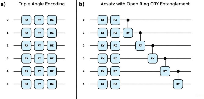 Figure 1
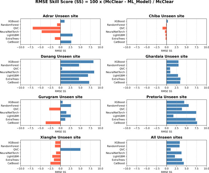 Figure 2
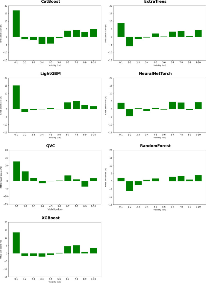 Figure 3
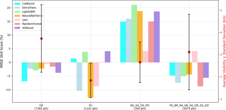 Figure 4
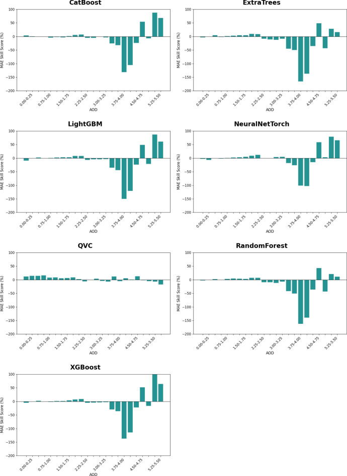 Figure 5
- —Deutsches Zentrum für Luft- und Raumfahrt e.V. (DLR) (4202)
Peer Reviews
No public reviews on file for this paper yet. If you reviewed it on a platform where reviews are public (OpenReview, ICLR, NeurIPS, ICML), you can paste yours below so the community can read it here.
Videos
No videos yet. Explain this paper in a talk, walkthrough, or lecture? Add one.
Taxonomy
TopicsSolar Radiation and Photovoltaics · Atmospheric aerosols and clouds · Photovoltaic System Optimization Techniques
Introduction
The integration of solar energy into the electricity grid presents unique challenges due to the fluctuating nature of solar irradiance, which can significantly affect power generation and grid stability. Accurate day-ahead and intra-day forecasts of all-sky global horizontal irradiance (GHI) are therefore essential: they support power system scheduling, reduce balancing costs, and help photovoltaic (PV) operators avoid penalties arising from forecast–production mismatches^1–3^. While day-ahead forecasts typically rely on numerical weather prediction (NWP), intra-day corrections are often derived from geostationary satellite imagery, which better provides more accurate cloud information due to the higher resolution^4,5^. Clouds remain the dominant source of irradiance variability^6^, but extreme aerosol events—such as dust storms, biomass burning, or urban smog—can also cause GHI reductions comparable to cloud cover^7–9^. These effects are particularly significant in tropical and subtropical regions, including the Indian subcontinent, eastern China, and Indochina, where some of the highest PV deployment rates coincide with frequent aerosol episodes^10–12^.
Estimating global horizontal clear-sky irradiance ( \documentclass[12pt]{minimal} \usepackage{amsmath} \usepackage{wasysym} \usepackage{amsfonts} \usepackage{amssymb} \usepackage{amsbsy} \usepackage{mathrsfs} \usepackage{upgreek} \setlength{\oddsidemargin}{-69pt} \begin{document}$${GHI}_{CS}$$\end{document} ) is a critical step for satellite-based all-sky GHI retrieval. Conventional approaches rely on aerosol optical depth (AOD) inputs for radiative transfer or empirical models^13,14^. Information on atmospheric aerosol concentration can be obtained at different spatio-temporal resolutions from satellite observations, numerical modelling, ground measurements or climatological datasets^15–18^. However, aerosol information is imperfect across all available sources. Satellite retrievals are limited by cloud contamination, choice of aerosol model and assumptions about aerosol properties^19^. Ground-based networks such as AERONET provide high-quality AOD measurements, but coverage is sparse and point-based observations are often unrepresentative^20,21^. Climatological datasets cannot capture rapid intra-day aerosol fluctuations^18^. A widely used tool for \documentclass[12pt]{minimal} \usepackage{amsmath} \usepackage{wasysym} \usepackage{amsfonts} \usepackage{amssymb} \usepackage{amsbsy} \usepackage{mathrsfs} \usepackage{upgreek} \setlength{\oddsidemargin}{-69pt} \begin{document}$${GHI}_{CS}$$\end{document} estimation is the McClear model^22^, which computes \documentclass[12pt]{minimal} \usepackage{amsmath} \usepackage{wasysym} \usepackage{amsfonts} \usepackage{amssymb} \usepackage{amsbsy} \usepackage{mathrsfs} \usepackage{upgreek} \setlength{\oddsidemargin}{-69pt} \begin{document}$${GHI}_{CS}$$\end{document} using AOD and other inputs from the Copernicus Atmosphere Monitoring Service (CAMS). McClear has been shown to perform well under many conditions globally^23^. However, it inherits the limitations of the CAMS aerosol data. CAMS provides global, hourly, 40 km–resolution fields and offers valuable large-scale coverage, but its spatial and temporal resolution makes it less suited to representing local or short-lived aerosol events. Regional assessments have reported systematic biases, such as underestimation of AOD in high-load conditions in Australia^24^, misrepresentation of fine-mode aerosols over the Indo-Gangetic Basin^25^, and inconsistencies in regions strongly influenced by biomass burning, desert dust, or mixed aerosol sources including Brazil and the Eastern Mediterranean^26–28^. Therefore, the following uncertainties can be identified with the different sources of aerosol information: (i) limitations in retrieval and numerical modelling algorithms, (ii) naïve aerosol constancy assumptions in climatology, and (iii) limited representativeness of sparsely available ground measurements.
Surface horizontal visibility has long been recognized as a proxy for aerosol extinction^29–35^, with early work such as the Elterman model^34^ establishing a link between visibility and vertical aerosol profiles. Modern retrievals have refined these methods with empirical corrections, optimization techniques, and calibration against satellite AOD products^36–40^. Although vertical visibility is more closely related to AOD, it is only reported when obscuring phenomena or ceiling conditions require a vertical measure, as recommended by WMO^41^. In contrast, horizontal visibility is routinely reported in METeorological Aerodrome Reports (METAR) at airports worldwide^42^, yielding a dense, near-real-time dataset that far surpasses the spatial coverage of dedicated aerosol networks^43–45^. Therefore, due to the sparse availability of vertical visibility measurements, it is not considered in this study and the term “visibility” henceforth will refer to horizontal visibility specifically. Visibility is influenced not only by aerosols but also by humidity, fog, precipitation, and wind^46–48^. As a result, its correlation with ground-based AOD is modest except under dust-dominated conditions^49,50^, and the interaction between AOD and relative humidity (RH) further complicates the relationship^51,52^. On its own, visibility is therefore insufficient as a direct substitute for AOD, but it holds promise when integrated with complementary datasets.
Machine learning (ML) offers a flexible framework for combining heterogeneous inputs and extracting non-linear relationships that elude traditional parameterizations^53,54^. Previous studies have applied tree-based models such as decision trees and random forests to estimate visibility from monthly or daily aerosol information and vice-versa^43,54^, but they fail to resolve rapid aerosol changes, leading to biased irradiance forecasts^55,56^. More advanced ML methods, including gradient boosting frameworks (e.g., XGBoost, LightGBM, CatBoost) and Neural Networks, offer improved performance, scalability, and robustness across diverse datasets^57–61^. Quantum variational circuits (QVCs) have also been proposed for ML applications^62,63^, though their application to solar energy meteorology remains largely exploratory. Despite these advances, few studies have systematically explored the integration of real-time visibility (METAR) with reanalysis products (CAMS) to improve clear-sky irradiance estimation.
This study addresses that gap with a data-driven framework for estimating \documentclass[12pt]{minimal} \usepackage{amsmath} \usepackage{wasysym} \usepackage{amsfonts} \usepackage{amssymb} \usepackage{amsbsy} \usepackage{mathrsfs} \usepackage{upgreek} \setlength{\oddsidemargin}{-69pt} \begin{document}$${GHI}_{CS}$$\end{document} . Specifically, It:
- Presents a data-driven approach using machine learning (ML) models for estimating global horizontal clear sky irradiance ( \documentclass[12pt]{minimal} \usepackage{amsmath} \usepackage{wasysym} \usepackage{amsfonts} \usepackage{amssymb} \usepackage{amsbsy} \usepackage{mathrsfs} \usepackage{upgreek} \setlength{\oddsidemargin}{-69pt} \begin{document}$${GHI}_{CS}$$\end{document} ) by combining METAR and CAMS aerosol datasets.
- Presents an approach for obtaining normalized pseudo global horizontal clear sky irradiance ( \documentclass[12pt]{minimal} \usepackage{amsmath} \usepackage{wasysym} \usepackage{amsfonts} \usepackage{amssymb} \usepackage{amsbsy} \usepackage{mathrsfs} \usepackage{upgreek} \setlength{\oddsidemargin}{-69pt} \begin{document}$${GHI}_{CS}^{*}$$\end{document} ) targets using ground measured GHI, satellite estimated cloud index (CI) and the top of atmosphere ( \documentclass[12pt]{minimal} \usepackage{amsmath} \usepackage{wasysym} \usepackage{amsfonts} \usepackage{amssymb} \usepackage{amsbsy} \usepackage{mathrsfs} \usepackage{upgreek} \setlength{\oddsidemargin}{-69pt} \begin{document}$${I}_{TOA}$$\end{document} ) irradiance, in order to compensate for the lack of direct measurements of \documentclass[12pt]{minimal} \usepackage{amsmath} \usepackage{wasysym} \usepackage{amsfonts} \usepackage{amssymb} \usepackage{amsbsy} \usepackage{mathrsfs} \usepackage{upgreek} \setlength{\oddsidemargin}{-69pt} \begin{document}$${GHI}_{CS}$$\end{document} in all-weather situations.
- Benchmarks the accuracy of satellite-estimated all-sky GHI derived using the \documentclass[12pt]{minimal} \usepackage{amsmath} \usepackage{wasysym} \usepackage{amsfonts} \usepackage{amssymb} \usepackage{amsbsy} \usepackage{mathrsfs} \usepackage{upgreek} \setlength{\oddsidemargin}{-69pt} \begin{document}$${GHI}_{CS}$$\end{document} output from the ML models utilizing METAR and CAMS data against the satellite-estimated all-sky GHI derived using the \documentclass[12pt]{minimal} \usepackage{amsmath} \usepackage{wasysym} \usepackage{amsfonts} \usepackage{amssymb} \usepackage{amsbsy} \usepackage{mathrsfs} \usepackage{upgreek} \setlength{\oddsidemargin}{-69pt} \begin{document}$${GHI}_{CS}$$\end{document} McClear model, at seven unseen sites.
- Validates the improvement in estimated all-sky GHI across a range of visibility situations and aerosol-related METAR weather codes.
- Validates the improvement in estimated all-sky GHI across a range of RH conditions.
Data and method
Ground measured GHI
Ground observations of GHI are obtained from eight stations located in regions strongly influenced by diverse aerosol conditions (Table 1). Data for Cairo, Gurgaon, Da Nang, Chiba, Adrar, Ghardaia and Pretoria are obtained from the CAMS Evaluation and Quality Control database hosted at Mines Paris^64^, while Xianghe measurements are retrieved via the BSRN FTP server^65^. The Cairo, Adrar, Ghardaia and Xianghe stations are equipped with Kipp & Zonen CMP21 secondary standard class A pyranometers, Gurgaon uses an Eppley PSP pyranometer, Da Nang is equipped with Huskeflux SR20 secondary standard class A pyranometer, Pretoria has a CMP11 secondary standard pyranometer and the Chiba SKYNET station employs a POM-01 sky radiometer. Table 1 provides a summary of the GHI measurement stations used in this study. All datasets are quality controlled using the open-source libinsitu software package developed under the International Energy Agency – Photovoltaic Power Systems Programme (IEA-PVPS) Task 16^64,66^. This includes removal of values flagged as invalid by the physical possible limit (PPL) and extremely rare limit tests. Following quality control, the GHI datasets are averaged from 1-min to 30-min resolution before being used in this study.Table 1. Stations providing GHI ground observations. SiteNetworkLocationSource of dataTime periodNative temporal resolution (min)Distance to next airport/METAR observation (km)CairoenerMENA30.04 ˚N, 31.01˚Ehttp://tds.webservice-energy.org/2015–2019139GurgaonBSRN28.42 ˚N, 77.16 ˚Ehttp://tds.webservice-energy.org/2018–2019112Da NangESMAP16.01 ˚N, 108.19 ˚Ehttp://tds.webservice-energy.org/2017–201918XiangheBSRN39.75 ˚N, 116.96 ˚Eftp://ftp.bsrn.awi.de/2010–2015171ChibaSKYNET35.63 ˚N, 140.10 ˚Ehttp://tds.webservice-energy.org/2015–2017120AdrarenerMENA27.88 ˚N, 0.27 ˚Whttp://tds.webservice-energy.org/2015–201619GhardaiaenerMENA32.39 ˚N, 3.78 ˚Ehttp://tds.webservice-energy.org/2015–201812PretoriaSAURAN25.75 ˚S, 28.23 ˚Ehttp://tds.webservice-energy.org/2015–202419
These stations are selected because they are located in regions characterized by frequent and diverse aerosol loading:
Cairo
Strongly affected by a mix of urban emissions, biomass burning, and desert dust^67^. Dust storms, especially in spring, contribute to high AOD and influence cloud properties^68^. A unique “urban haze” composed of submicron ammonium chloride (from biomass burning) and super micron dust has been reported^69^.
Gurgaon (near Delhi)
High aerosol concentrations result from industrial-vehicular emissions, biomass burning and dust storms, with significant seasonal variations. Biomass burning dominates in the post-monsoon and winter periods^70,71^, industrial emissions persist year-round with peaks after monsoon^72^ and dust storms are common during pre-monsoon and monsoon^73^.
Xianghe (near Beijing)
Summer exhibits the highest AOD and fine-mode fraction due to urban haze^74^, winter has moderate AOD with increased coarse-mode aerosols from heating activities^75^, and spring is influenced by desert dust^74^.
Chiba (near Tokyo)
Organic aerosols dominate composition (40 – 60%) across seasons, with daytime peaks^76^. Diesel exhaust is a major source of fine particulate matter^77^.
Da Nang
Rice straw burning during late summer-autumn harvests elevates PM_2.5_ and NO_2_^78^. Such practices are most prevalent during the harvest season from late summer to early autumn. Black carbon from quarrying and vehicular pollution peaks in the dry season (June – July)^79^.
Adrar
The Adrar plateau is a significant dust source region^80^. Existing studies have found elevated atmospheric turbidity in summer period due to a low cohesion of sand/dust particles caused by higher ambient temperature and lower relative humidity, accompanied with stronger winds that can transport sand and dust particles^81^.
Ghardaia
Hot weather and Sirocco winds result in increased dust/ sand aerosol during summer^82^. Prone to urban aerosols due to the prevalence of mining-related crusher plants in the area^83^.
Pretoria
Elevated atmospheric aerosol concentration due to anthropogenic sources of air pollution, particularly due to bio-fuel burning in winter^84^. Atmospheric brown clouds with large amounts of absorbing aerosols, including black carbon, are frequently observed^85^.
Cloud observations from satellites
Surface Solar Radiation Data Set – Heliosat (SARAH-3)^86^, available at 30-min temporal resolution on a 0.05˚ × 0.05˚ regular grid, is generated by applying the MAGICSOL algorithm on the images from Meteosat Second Generation (MSG2), located at 0 ˚E. MAGICSOL derives the effective cloud albedo (CAL) using the original Heliosat method^87^.
The Heliosat method is a widely-used approach for estimating surface solar irradiance from satellite imagery, based on the relationship between cloud optical properties and solar radiation attenuation. The method exploits the principle that satellite-observed reflectance is inversely related to ground-level irradiance: bright (cloudy) pixels correspond to lower surface irradiance, while dark (clear-sky) pixels indicate higher irradiance. Heliosat-1^88^, -2^89^, and -3^90^ employ a normalization technique (shown in Eq. 1) to convert satellite-measured reflectance into CI, followed by the empirical relation in Eq. 2 to convert CI into clear-sky index \documentclass[12pt]{minimal} \usepackage{amsmath} \usepackage{wasysym} \usepackage{amsfonts} \usepackage{amssymb} \usepackage{amsbsy} \usepackage{mathrsfs} \usepackage{upgreek} \setlength{\oddsidemargin}{-69pt} \begin{document}$${k}_{c}$$\end{document} (the ratio of GHI to \documentclass[12pt]{minimal} \usepackage{amsmath} \usepackage{wasysym} \usepackage{amsfonts} \usepackage{amssymb} \usepackage{amsbsy} \usepackage{mathrsfs} \usepackage{upgreek} \setlength{\oddsidemargin}{-69pt} \begin{document}$$GH{I}_{CS}$$\end{document} ). GHI is subsequently derived by multiplying \documentclass[12pt]{minimal} \usepackage{amsmath} \usepackage{wasysym} \usepackage{amsfonts} \usepackage{amssymb} \usepackage{amsbsy} \usepackage{mathrsfs} \usepackage{upgreek} \setlength{\oddsidemargin}{-69pt} \begin{document}$${k}_{c}$$\end{document} with \documentclass[12pt]{minimal} \usepackage{amsmath} \usepackage{wasysym} \usepackage{amsfonts} \usepackage{amssymb} \usepackage{amsbsy} \usepackage{mathrsfs} \usepackage{upgreek} \setlength{\oddsidemargin}{-69pt} \begin{document}$$GH{I}_{CS}$$\end{document} from a clear sky model. These empirical versions differ primarily in the calibration of reference surface albedo \documentclass[12pt]{minimal} \usepackage{amsmath} \usepackage{wasysym} \usepackage{amsfonts} \usepackage{amssymb} \usepackage{amsbsy} \usepackage{mathrsfs} \usepackage{upgreek} \setlength{\oddsidemargin}{-69pt} \begin{document}$${\rho }_{g}$$\end{document} and cloud albedo \documentclass[12pt]{minimal} \usepackage{amsmath} \usepackage{wasysym} \usepackage{amsfonts} \usepackage{amssymb} \usepackage{amsbsy} \usepackage{mathrsfs} \usepackage{upgreek} \setlength{\oddsidemargin}{-69pt} \begin{document}$${\rho }_{c}$$\end{document} . However, they all share the same fundamental concept of estimating atmospheric transmittance through satellite-observed reflectance.Table 2. Satellite-estimated products used in this study.Site nameSatellite product nameSourceCairoCloud albedoOnline repository of the Satellite Application Facility (CM-SAF) on Climate Monitoring, SARAH-3 datasetAdrarCloud albedoOnline repository of the Satellite Application Facility (CM-SAF) on Climate Monitoring, SARAH-3 datasetGhardaiaCloud albedoOnline repository of the Satellite Application Facility (CM-SAF) on Climate Monitoring, SARAH-3 datasetPretoriaCloud albedoOnline repository of the Satellite Application Facility (CM-SAF) on Climate Monitoring, SARAH-3 datasetGurgaonCloud opacitySolcast web platform and APIDa NangCloud opacitySolcast web platform and APIXiangheCloud opacitySolcast web platform and APIChibaCloud opacitySolcast web platform and API
\documentclass[12pt]{minimal} \usepackage{amsmath} \usepackage{wasysym} \usepackage{amsfonts} \usepackage{amssymb} \usepackage{amsbsy} \usepackage{mathrsfs} \usepackage{upgreek} \setlength{\oddsidemargin}{-69pt} \begin{document}$$\begin{array}{c}CI=\frac{\left(\rho -{\rho }_{g}\right)}{\left({\rho }_{c}-{\rho }_{g}\right)}\end{array}$$\end{document}In the SARAH-3 dataset, CAL is the variable corresponding to CI. For this study, CAL values for the Cairo station (30.04 ˚N, 31.01 ˚E) are extracted via spatial interpolation for the time period 2015–2019 (Table 1), which corresponds to the openly available reference data from the stations under IEA-PVPS Task 16. Similarly, CAL values for Adrar, Ghardaia and Pretoria (Table 2) are also extracted via spatial interpolation for the respective time periods mentioned in (Table 1). CAL is converted to clear sky index ( \documentclass[12pt]{minimal} \usepackage{amsmath} \usepackage{wasysym} \usepackage{amsfonts} \usepackage{amssymb} \usepackage{amsbsy} \usepackage{mathrsfs} \usepackage{upgreek} \setlength{\oddsidemargin}{-69pt} \begin{document}$${k}_{c}$$\end{document} ) following the procedure in^91^, summarized in Eq. (2).
\documentclass[12pt]{minimal} \usepackage{amsmath} \usepackage{wasysym} \usepackage{amsfonts} \usepackage{amssymb} \usepackage{amsbsy} \usepackage{mathrsfs} \usepackage{upgreek} \setlength{\oddsidemargin}{-69pt} \begin{document}$$\begin{array}{c}{k}_{c}=\left\{\begin{array}{c}1.2, {\mathrm{f}}{\mathrm{o}}{\mathrm{r}} CI\le -0.2\\ 1-CI, {\mathrm{f}}{\mathrm{o}}{\mathrm{r}}-0.2\le CI\le 0.8\\ 1.661-1.7814CI+0.7250{CI}^{2}, {\mathrm{f}}{\mathrm{o}}{\mathrm{r}} 0.8\le CI\le 1.05\\ 0.09, {\mathrm{f}}{\mathrm{o}}{\mathrm{r}} 1.05<CI\end{array}\right\}\end{array}$$\end{document}where,
\documentclass[12pt]{minimal} \usepackage{amsmath} \usepackage{wasysym} \usepackage{amsfonts} \usepackage{amssymb} \usepackage{amsbsy} \usepackage{mathrsfs} \usepackage{upgreek} \setlength{\oddsidemargin}{-69pt} \begin{document}$${k}_{c}:$$\end{document} clear sky index
\documentclass[12pt]{minimal} \usepackage{amsmath} \usepackage{wasysym} \usepackage{amsfonts} \usepackage{amssymb} \usepackage{amsbsy} \usepackage{mathrsfs} \usepackage{upgreek} \setlength{\oddsidemargin}{-69pt} \begin{document}$$CI:$$\end{document} cloud index
Complementary datasets of cloud opacity at 30-min resolution for Xianghe, Chiba, Gurgaon and Da Nang (Table 2) are obtained from the Solcast platform^92^. Solcast does not release the full details of its proprietary methodology; however, published studies indicate that its approach is based on semi-empirical retrievals of cloud properties from geostationary satellite imagery^93^. In line with prior literature^94^, cloud opacity is considered equivalent to CI (or CAL), and is therefore converted to \documentclass[12pt]{minimal} \usepackage{amsmath} \usepackage{wasysym} \usepackage{amsfonts} \usepackage{amssymb} \usepackage{amsbsy} \usepackage{mathrsfs} \usepackage{upgreek} \setlength{\oddsidemargin}{-69pt} \begin{document}$${k}_{c}$$\end{document} using Eq. ( \documentclass[12pt]{minimal} \usepackage{amsmath} \usepackage{wasysym} \usepackage{amsfonts} \usepackage{amssymb} \usepackage{amsbsy} \usepackage{mathrsfs} \usepackage{upgreek} \setlength{\oddsidemargin}{-69pt} \begin{document}$$2$$\end{document} ).
Aerosols and other atmospheric parameters
McClear clear sky irradiance and CAMS aerosol
\documentclass[12pt]{minimal} \usepackage{amsmath} \usepackage{wasysym} \usepackage{amsfonts} \usepackage{amssymb} \usepackage{amsbsy} \usepackage{mathrsfs} \usepackage{upgreek} \setlength{\oddsidemargin}{-69pt} \begin{document}$${GHI}_{CS}$$\end{document} For the sites used in this study are obtained from the McClear service of CAMS^22^. The atmospheric composition input into the McClear model comes from the CAMS EAC4 global reanalysis prior to 2023–07^95^, which has a spatial resolution of 0.75° × 0.75° and a temporal resolution of 3 h. The McClear model uses inputs from the CAMS global atmospheric composition forecast from 2023–07 onwards, which has a spatial resolution of 0.35° × 0.35° and a temporal resolution of 3 h^96^. In addition, McClear internally calculates solar geometry parameters and top of atmosphere irradiance ( \documentclass[12pt]{minimal} \usepackage{amsmath} \usepackage{wasysym} \usepackage{amsfonts} \usepackage{amssymb} \usepackage{amsbsy} \usepackage{mathrsfs} \usepackage{upgreek} \setlength{\oddsidemargin}{-69pt} \begin{document}$${I}_{TOA}$$\end{document} ). For this study, McClear \documentclass[12pt]{minimal} \usepackage{amsmath} \usepackage{wasysym} \usepackage{amsfonts} \usepackage{amssymb} \usepackage{amsbsy} \usepackage{mathrsfs} \usepackage{upgreek} \setlength{\oddsidemargin}{-69pt} \begin{document}$${GHI}_{CS}$$\end{document} and the same atmospheric composition data used by McClear (CAMS EAC4 for the period before 2023–07 and CAMS global atmospheric composition forecasts for the period after 2023–07) are retrieved for each site with the Climate Data Store Applications Program Interface (cdsapi). Outputs are requested at 30-min temporal resolution, consistent with the temporal resolution of the METAR data. As CAMS reanalysis is available at 3 hourly resolution, the 30-min values are obtained by assuming constant atmospheric conditions within each 3 h window. The full list of parameters used in this study is summarized in (Table 3).Table 3. Summary of the CAMS global reanalysis parameters used in this study.ParameterDescription \documentclass[12pt]{minimal} \usepackage{amsmath} \usepackage{wasysym} \usepackage{amsfonts} \usepackage{amssymb} \usepackage{amsbsy} \usepackage{mathrsfs} \usepackage{upgreek} \setlength{\oddsidemargin}{-69pt} \begin{document}$${I}_{TOA}$$\end{document} Irradiation on a horizontal plane at the top of atmosphereszaSolar zenith angle in degreestco3Total column content of ozone in Dobson unittcwvTotal column content of water vapour in kg/m^2^AODTotal aerosol optical depth at 550 nm
METAR
METAR recorded atmospheric parameters observed once every 30 min are obtained for the closest airport to the eight sites. The International Civil Aviation Organization (ICAO) mandates automated visibility measurements from transmissometers or forward scatter meters for all airports which have runways where Category (CAT) II and CAT III Instrumented Landing Systems (ILS) are used^97^. For runways using ILS CAT I, automated visibility measurements are also recommended. The datasets shown in Table 4 are downloaded from the Iowa Environmental Mesonet repository^98^ maintained by the Iowa State University of Science and Technology, which has a long-term archive of airport Automated Surface/ Weather Observation Stations (ASOS/AWOS) for weather parameters. The temperature, wind speed and visibility measurements are converted to SI units, i.e., ˚C, m/s and km. Visibility measurements at airports commonly use transmissometers and forwards scatter sensors for METAR reports^99^. Quality checks involve comparing sensor data with human observations and reference instruments.Table 4. Atmospheric parameters from METAR data.ParameterDescriptionrelhRH in %vsbyVisibility in mileswxcodesSignificant weather observations
Furthermore, METAR provides observations of the significant weather. Namely, the classes Haze (HZ), Smoke (FU), Widespread Dust (DU), Sand (SA), Sandstorm (SS), Duststorm (DS) and Dust/ Sand whirls (PO) are related to aerosols and are used for diagnostic classification of the results.
Machine learning setup
In this study, a group of ML models (described in Sect. 3.4) are used to directly estimate a normalized pseudo global horizontal clear sky irradiance (explained in Sect. 3.3) with chosen CAMS Reanalysis and METAR parameters (described in Sect. 3.2). This essentially combines the (i) Visibility to AOD, and (ii) AOD to Clear sky irradiance conversion steps into one, and avoids the need for a separate Visibility to AOD conversion methodology.
Training-validation-test data split
Cairo is a site with a large number of data points and is characterized both by dust and anthropogenic pollution conditions. Therefore, it is chosen for the development of the ML models.
Two-third of the available datapoints from Cairo, as shown in (Table 5) are used for training the models and the remaining one-third for validation and hyperparameter tuning. The training-validation split is not done randomly but in a chronological manner, to ensure that different datapoints from the same days do not appear in the training and validation datasets. Otherwise, due to similarity in the atmospheric situation over a day, the model may produce memorized results instead of learning. The data from the remaining seven sites are used to test the performance of the model on previously unseen sites. This is done to check whether the trained models are able to overcome site-dependency.Table 5. Availability of quality controlled datapoints for the analysis.SiteQuality checked datapointsTraining and validationTestingCairo20,914-Gurgaon-6,222Da Nang-12,800Xianghe-16,268Chiba-14,682Adrar-13,640Ghardaia-20,430Pretoria-65,560
Predictor preparation
In order to reduce the computational load, the CAMS AOD values of the different species at 550 nm are not entered simultaneously as inputs into the models. Instead, the (i) total AOD at 550 nm is used in this analysis. Further input parameters into the ML models are selected as follows: (ii) Visibility measurements from airport, which provide local information on the atmospheric aerosol loading at the surface. (iii) RH, as it is correlated to the presence of fog and mist, which are known to occur with smog. (iv) Solar zenith angle (SZA), as the cosine of SZA is inversely proportional to the air mass that \documentclass[12pt]{minimal} \usepackage{amsmath} \usepackage{wasysym} \usepackage{amsfonts} \usepackage{amssymb} \usepackage{amsbsy} \usepackage{mathrsfs} \usepackage{upgreek} \setlength{\oddsidemargin}{-69pt} \begin{document}$${I}_{TOA}$$\end{document} travels through and undergoes dissipation before reaching the surface. (v) Solar azimuth angle, as it is correlated to the diurnal movement of the Sun. (vi) Total column water vapour (TCWV), as it is found to be a significant contributor to the reduction of GHI and the dissipative effect increases with the increase in SZA^100^.
Target preparation
The cloud-free component of irradiance in all-sky situations cannot be measured directly. GHI measurements taken during cloudless periods are equivalent to \documentclass[12pt]{minimal} \usepackage{amsmath} \usepackage{wasysym} \usepackage{amsfonts} \usepackage{amssymb} \usepackage{amsbsy} \usepackage{mathrsfs} \usepackage{upgreek} \setlength{\oddsidemargin}{-69pt} \begin{document}$${GHI}_{CS}$$\end{document} . Various approaches for filtering clear sky situations are found in the literature, and the majority of them uses a clear sky model or requires all three components of solar irradiance or use some statistical approaches^101–103^. While the filtering step greatly reduces the number of datapoints available for training and validation, it also risks removing events where irradiance decreases because of aerosols rather than clouds. This occurs because aerosol-driven irradiance drops can be misclassified as cloudy conditions, particularly during dust storms or smog episodes where aerosols and clouds often co-occur. Furthermore, as \documentclass[12pt]{minimal} \usepackage{amsmath} \usepackage{wasysym} \usepackage{amsfonts} \usepackage{amssymb} \usepackage{amsbsy} \usepackage{mathrsfs} \usepackage{upgreek} \setlength{\oddsidemargin}{-69pt} \begin{document}$${GHI}_{CS}$$\end{document} is finally used for deriving satellite-estimated GHI from CI in both clear and cloudy situations, it is necessary to evaluate its performance also in both situations. Due to these reasons, no explicit separation of clear sky and cloudy sky datapoints are performed in this study. Instead, a normalized pseudo global horizontal clear sky irradiance ( \documentclass[12pt]{minimal} \usepackage{amsmath} \usepackage{wasysym} \usepackage{amsfonts} \usepackage{amssymb} \usepackage{amsbsy} \usepackage{mathrsfs} \usepackage{upgreek} \setlength{\oddsidemargin}{-69pt} \begin{document}$${GHI}_{CS}^{*}$$\end{document} ) is derived, starting from the expression of \documentclass[12pt]{minimal} \usepackage{amsmath} \usepackage{wasysym} \usepackage{amsfonts} \usepackage{amssymb} \usepackage{amsbsy} \usepackage{mathrsfs} \usepackage{upgreek} \setlength{\oddsidemargin}{-69pt} \begin{document}$${GHI}_{CS}$$\end{document} at ground level shown in Eq. 3.
\documentclass[12pt]{minimal} \usepackage{amsmath} \usepackage{wasysym} \usepackage{amsfonts} \usepackage{amssymb} \usepackage{amsbsy} \usepackage{mathrsfs} \usepackage{upgreek} \setlength{\oddsidemargin}{-69pt} \begin{document}$$\begin{array}{c}GH{I}_{CS}=\frac{GHI}{{k}_{c}}\approx \frac{GH{I}_{ground}}{\left(1-n\right)}\end{array}$$\end{document}where,
\documentclass[12pt]{minimal} \usepackage{amsmath} \usepackage{wasysym} \usepackage{amsfonts} \usepackage{amssymb} \usepackage{amsbsy} \usepackage{mathrsfs} \usepackage{upgreek} \setlength{\oddsidemargin}{-69pt} \begin{document}$$GH{I}_{ground}:$$\end{document} ground measured GHI
\documentclass[12pt]{minimal} \usepackage{amsmath} \usepackage{wasysym} \usepackage{amsfonts} \usepackage{amssymb} \usepackage{amsbsy} \usepackage{mathrsfs} \usepackage{upgreek} \setlength{\oddsidemargin}{-69pt} \begin{document}$${k}_{c}:$$\end{document} clear sky index
\documentclass[12pt]{minimal} \usepackage{amsmath} \usepackage{wasysym} \usepackage{amsfonts} \usepackage{amssymb} \usepackage{amsbsy} \usepackage{mathrsfs} \usepackage{upgreek} \setlength{\oddsidemargin}{-69pt} \begin{document}$${GHI}_{CS}:$$\end{document} clear sky GHI
\documentclass[12pt]{minimal} \usepackage{amsmath} \usepackage{wasysym} \usepackage{amsfonts} \usepackage{amssymb} \usepackage{amsbsy} \usepackage{mathrsfs} \usepackage{upgreek} \setlength{\oddsidemargin}{-69pt} \begin{document}$$n$$\end{document} : satellite estimated cloud index or cloud opacity
\documentclass[12pt]{minimal} \usepackage{amsmath} \usepackage{wasysym} \usepackage{amsfonts} \usepackage{amssymb} \usepackage{amsbsy} \usepackage{mathrsfs} \usepackage{upgreek} \setlength{\oddsidemargin}{-69pt} \begin{document}$$GH{I}_{ground}$$\end{document} is obtained from surface measurements and CI from satellite images. Of course, this equation will not hold true for situations where the cloudiness seen by the pyranometer at the surface level does not match the cloudiness seen from satellite. This could be due to the effects of parallax and cloud shadow displacement, in which case systematic biases depending on sun position (time of day), cloud height and site location with respect to the satellite, are expected^104^. This could also be due to the limitations in cloud resolving capability because of the relatively coarse spatial resolution of satellite pixels, in which case random outliers are expected^105^. However, it is expected that the statistics-based machine learning methods will be able to handle these outlier situations. Furthermore, the above expression is normalized by \documentclass[12pt]{minimal} \usepackage{amsmath} \usepackage{wasysym} \usepackage{amsfonts} \usepackage{amssymb} \usepackage{amsbsy} \usepackage{mathrsfs} \usepackage{upgreek} \setlength{\oddsidemargin}{-69pt} \begin{document}$${I}_{TOA}$$\end{document} in order to restrict the \documentclass[12pt]{minimal} \usepackage{amsmath} \usepackage{wasysym} \usepackage{amsfonts} \usepackage{amssymb} \usepackage{amsbsy} \usepackage{mathrsfs} \usepackage{upgreek} \setlength{\oddsidemargin}{-69pt} \begin{document}$${GHI}_{CS}^{*}$$\end{document} values within the range \documentclass[12pt]{minimal} \usepackage{amsmath} \usepackage{wasysym} \usepackage{amsfonts} \usepackage{amssymb} \usepackage{amsbsy} \usepackage{mathrsfs} \usepackage{upgreek} \setlength{\oddsidemargin}{-69pt} \begin{document}$$\left[\mathrm{0,1}\right]$$\end{document} , as shown in Eq. 4, which is more efficient for training ML models. Overshooting of GHI values beyond \documentclass[12pt]{minimal} \usepackage{amsmath} \usepackage{wasysym} \usepackage{amsfonts} \usepackage{amssymb} \usepackage{amsbsy} \usepackage{mathrsfs} \usepackage{upgreek} \setlength{\oddsidemargin}{-69pt} \begin{document}$${I}_{TOA}$$\end{document} due to cloud enhancement are neglected in this approach, which is justified by the 30 min averages of GHI analyzed.
\documentclass[12pt]{minimal} \usepackage{amsmath} \usepackage{wasysym} \usepackage{amsfonts} \usepackage{amssymb} \usepackage{amsbsy} \usepackage{mathrsfs} \usepackage{upgreek} \setlength{\oddsidemargin}{-69pt} \begin{document}$$\begin{array}{c}Target=\frac{GH{I}_{clear}}{{I}_{TOA}}=\frac{GH{I}_{ground}}{\left(\left(1-n\right)\times {I}_{TOA}\right)}\end{array}$$\end{document}Machine learning models
Popular models for multi-variate regression are used in this analysis, including gradient boosting methods – (i) XGBoost, (ii) LightGBM, (iii) CatBoost, tree-based methods – (iv) Extra Trees, (v) Random Forest, and (vi) Neural Network. Furthermore, a more recent approach of using QVC for machine learning has also been explored. The following subsections provide a brief description of each model.
EXtreme gradient boosting (XGBoost)
XGBoost leverages the principles of boosting ensemble techniques to enhance prediction accuracy. It operates on the premise of sequentially adding weak learners (typically decision trees) to improve the performance of the overall model. XGBoost employs a unique regularization approach and handles missing values internally while optimizing computation speed and model robustness through parallel processing. An efficient and scalable Python implementation of XGBoost published by the original authors has been used in this analysis^106^.
Light gradient-boosting machine (LightGBM)
LightGBM, developed by Microsoft, improves upon traditional gradient boosting frameworks by integrating Gradient-based One-Side Sampling (GOSS) and Exclusive Feature Bundling (EFB) techniques. These innovations allow LightGBM to handle vast datasets effectively while reducing memory usage and computation time. Similar to XGBoost, LightGBM uses a decision-tree-based learning algorithm but optimizes the training process by exclusively focusing on the gradients of the chosen data subset. The latest version of the official LightGBM python implementation from Microsoft is used in this analysis^107^.
Categorical boosting (CatBoost)
CaBoost is a gradient boosting algorithm that uses ordered boosting to reduce prediction shift and target leakage^108^. In several studies, CatBoost achieved competitive or enhanced accuracy on tasks with imbalanced or categorical data, although its training speed was generally slower than that of LightGBM and XGBoost^109^.
Random forest
Random Forests combine many decision trees to improve predictions^110^. Random Forests build trees by drawing bootstrap samples and choosing splits that optimize measures such as impurity or variance reduction.
Extremely randomized trees (Extra-Trees)
Extra-Trees averages the predictions from multiple decision trees, obtained by portioning the input-space with randomly generated splits^111^. However, Extra-Trees work on the full training set and select both the splitting feature and the split point at random^60^. Empirical work indicates that in high-dimensional or noisy settings Extra-Trees may match or exceed the performance of Random Forests.
Neural network (NeuralNetTorch)
Neural network consists of multiple layers of perceptrons or neurons, which learn to transform input data into desired output through a process of weighted connections. It utilizes backpropagation to adjust the weights based on the error between predicted and actual outputs, which facilitates learning intricate patterns in data. PyTorch implementation of Neural Network is used in this analysis^112^.
Quantum variational circuit (QVC)
QVCs encode classical data into quantum states and employ a parameterized quantum circuit (ansatz) to produce the predictions^93^. The data encoder circuit determines the frequency spectrum of the quantum model, which in turn affects its expressivity and thereby its ability to learn different types of functions^76^. In this study, a feature encoder with learnable parameters is used, as shown in Fig. 1, for the chosen input predictors \documentclass[12pt]{minimal} \usepackage{amsmath} \usepackage{wasysym} \usepackage{amsfonts} \usepackage{amssymb} \usepackage{amsbsy} \usepackage{mathrsfs} \usepackage{upgreek} \setlength{\oddsidemargin}{-69pt} \begin{document}$${x}_{m}$$\end{document} . The inputs are encoded through parameterized rotations \documentclass[12pt]{minimal} \usepackage{amsmath} \usepackage{wasysym} \usepackage{amsfonts} \usepackage{amssymb} \usepackage{amsbsy} \usepackage{mathrsfs} \usepackage{upgreek} \setlength{\oddsidemargin}{-69pt} \begin{document}$${R}_{X}\left({\theta }_{mX}\cdot {x}_{m}\right)$$\end{document} , \documentclass[12pt]{minimal} \usepackage{amsmath} \usepackage{wasysym} \usepackage{amsfonts} \usepackage{amssymb} \usepackage{amsbsy} \usepackage{mathrsfs} \usepackage{upgreek} \setlength{\oddsidemargin}{-69pt} \begin{document}$${R}_{Y}\left({\theta }_{mY}\cdot {x}_{m}\right)$$\end{document} and \documentclass[12pt]{minimal} \usepackage{amsmath} \usepackage{wasysym} \usepackage{amsfonts} \usepackage{amssymb} \usepackage{amsbsy} \usepackage{mathrsfs} \usepackage{upgreek} \setlength{\oddsidemargin}{-69pt} \begin{document}$${R}_{Z}\left({\theta }_{mZ}\cdot {x}_{m}\right)$$\end{document} , as it has been shown that angle encoding with learnable parameters can help reduce circuit depth^113^. \documentclass[12pt]{minimal} \usepackage{amsmath} \usepackage{wasysym} \usepackage{amsfonts} \usepackage{amssymb} \usepackage{amsbsy} \usepackage{mathrsfs} \usepackage{upgreek} \setlength{\oddsidemargin}{-69pt} \begin{document}$${\theta }_{mX}$$\end{document} , \documentclass[12pt]{minimal} \usepackage{amsmath} \usepackage{wasysym} \usepackage{amsfonts} \usepackage{amssymb} \usepackage{amsbsy} \usepackage{mathrsfs} \usepackage{upgreek} \setlength{\oddsidemargin}{-69pt} \begin{document}$${\theta }_{mY}$$\end{document} and \documentclass[12pt]{minimal} \usepackage{amsmath} \usepackage{wasysym} \usepackage{amsfonts} \usepackage{amssymb} \usepackage{amsbsy} \usepackage{mathrsfs} \usepackage{upgreek} \setlength{\oddsidemargin}{-69pt} \begin{document}$${\theta }_{mZ}$$\end{document} are the learnable rotation parameters corresponding to the input feature \documentclass[12pt]{minimal} \usepackage{amsmath} \usepackage{wasysym} \usepackage{amsfonts} \usepackage{amssymb} \usepackage{amsbsy} \usepackage{mathrsfs} \usepackage{upgreek} \setlength{\oddsidemargin}{-69pt} \begin{document}$${x}_{m}$$\end{document} .Fig. 1(a) Data encoder layer and (b) Ansatz of the quantum variational circuit.
Results and discussion
As already mentioned, it is not straightforward to evaluate the quality of \documentclass[12pt]{minimal} \usepackage{amsmath} \usepackage{wasysym} \usepackage{amsfonts} \usepackage{amssymb} \usepackage{amsbsy} \usepackage{mathrsfs} \usepackage{upgreek} \setlength{\oddsidemargin}{-69pt} \begin{document}$${GHI}_{CS}$$\end{document} estimates in all-sky situations because \documentclass[12pt]{minimal} \usepackage{amsmath} \usepackage{wasysym} \usepackage{amsfonts} \usepackage{amssymb} \usepackage{amsbsy} \usepackage{mathrsfs} \usepackage{upgreek} \setlength{\oddsidemargin}{-69pt} \begin{document}$${GHI}_{CS}$$\end{document} cannot be directly measured in cloudy situations. Therefore, the \documentclass[12pt]{minimal} \usepackage{amsmath} \usepackage{wasysym} \usepackage{amsfonts} \usepackage{amssymb} \usepackage{amsbsy} \usepackage{mathrsfs} \usepackage{upgreek} \setlength{\oddsidemargin}{-69pt} \begin{document}$${GHI}_{CS}$$\end{document} estimates obtained from the ML models are evaluated by using them in the Heliosat-3 method and validating the accuracy of satellite-estimated all-sky GHI derived from them against the ground measured GHI. \documentclass[12pt]{minimal} \usepackage{amsmath} \usepackage{wasysym} \usepackage{amsfonts} \usepackage{amssymb} \usepackage{amsbsy} \usepackage{mathrsfs} \usepackage{upgreek} \setlength{\oddsidemargin}{-69pt} \begin{document}$${GHI}_{CS}$$\end{document} from the physics-based McClear model, which utilizes CAMS AOD, is also used in the Heliosat-3 method to produce satellite-estimated all-sky GHI, and is used as a reference benchmark. All GHI datasets are averaged to 30 min resolution, prior to validation.
The general performance for all the test datapoints used in this analysis is evaluated using the coefficient of determination (R^2^), the root mean square error (RMSE), the mean absolute error (MAE) and the mean bias error (MBE), shown in Eqs. 5, 6, 7 and 8 respectively. The R^2^ metric gives an idea about the overall fit of the estimated values compared to the measured values. RMSE shows the average deviation of the estimated values with strong emphasis on large errors. The utility of the additional METAR data is analyzed by evaluating the percentage improvement in RMSE due to the ML models in comparison to the McClear model, across the available range of visibility values.
\documentclass[12pt]{minimal} \usepackage{amsmath} \usepackage{wasysym} \usepackage{amsfonts} \usepackage{amssymb} \usepackage{amsbsy} \usepackage{mathrsfs} \usepackage{upgreek} \setlength{\oddsidemargin}{-69pt} \begin{document}$${R}^{2}=1-{\sum }_{i=1}^{n}\frac{{\left({y}_{target}^{i}-{y}_{model}^{i}\right)}^{2}}{{\left({y}_{target}^{i}-\frac{1}{n}{\sum }_{i=1}^{n}{y}_{target}^{i}\right)}^{2}}$$\end{document} \documentclass[12pt]{minimal} \usepackage{amsmath} \usepackage{wasysym} \usepackage{amsfonts} \usepackage{amssymb} \usepackage{amsbsy} \usepackage{mathrsfs} \usepackage{upgreek} \setlength{\oddsidemargin}{-69pt} \begin{document}$$RMSE =\sqrt{\frac{1}{n}{\sum }_{i=1}^{N}{\left({y}_{model}^{i}-{y}_{target}^{i}\right)}^{2}}$$\end{document} \documentclass[12pt]{minimal} \usepackage{amsmath} \usepackage{wasysym} \usepackage{amsfonts} \usepackage{amssymb} \usepackage{amsbsy} \usepackage{mathrsfs} \usepackage{upgreek} \setlength{\oddsidemargin}{-69pt} \begin{document}$$MAE =\frac{1}{n}{\sum }_{i=1}^{N}\left|{y}_{model}^{i}-{y}_{target}^{i}\right|$$\end{document} \documentclass[12pt]{minimal} \usepackage{amsmath} \usepackage{wasysym} \usepackage{amsfonts} \usepackage{amssymb} \usepackage{amsbsy} \usepackage{mathrsfs} \usepackage{upgreek} \setlength{\oddsidemargin}{-69pt} \begin{document}$$MBE =\frac{1}{n}{\sum }_{i=1}^{N}\left({y}_{model}^{i}-{y}_{target}^{i}\right)$$\end{document}The overall all-sky RMSE in Heliosat-3 estimated GHI using the \documentclass[12pt]{minimal} \usepackage{amsmath} \usepackage{wasysym} \usepackage{amsfonts} \usepackage{amssymb} \usepackage{amsbsy} \usepackage{mathrsfs} \usepackage{upgreek} \setlength{\oddsidemargin}{-69pt} \begin{document}$${GHI}_{CS}$$\end{document} values obtained from ML models, are slightly reduced compared to the RMSE when \documentclass[12pt]{minimal} \usepackage{amsmath} \usepackage{wasysym} \usepackage{amsfonts} \usepackage{amssymb} \usepackage{amsbsy} \usepackage{mathrsfs} \usepackage{upgreek} \setlength{\oddsidemargin}{-69pt} \begin{document}$${GHI}_{CS}$$\end{document} obtained from McClear is used (Fig. 2). Out of the models tested in this study, CatBoost shows the highest RMSE Skill Score (SS) on an overall basis. While the QVC shows the least RMSE SS, it must also be considered that it uses a very low number of learnable parameters (188) in comparison to the other models such as the Neural Network (which uses 50561 learnable parameters). Also, the number of layers had to be restricted due to the computational requirements. Most of the ML models did not perform well at the Xinaghe and Chiba sites. The visibility measurement station is inside the Beijing airport close to the city while the GHI measurement station is 71 km away in Xianghe (shown in Table 1), which is less urbanized. The large distance and the difference in built environment presumably results in lower correlation in atmospheric aerosol composition and concentration between the two sites^114^. Similarly for the Chiba site, only the XGBoost model showed improvement relative to McClear. Here again, the visibility measurement site is inside Tokyo airport, which is located in the highly urbanized Inner Bay area. The GHI measurement site is located in Chiba, which has significantly lower built-up area compared to Tokyo Inner Bay^115^. Considerable differences in aerosol type and composition have been reported between these two areas^116^. The relatively poor performance of the ML models at the Xianghe and Chiba sites could therefore be attributed to the differences in micro-climate between the visibility and GHI measurement sites for these two locations, which leads to lower correlation in atmospheric aerosol composition and concentration. The R^2^ metric (Table 6) shows that the accuracy of the all-sky GHI derived using different ML models and McClear, are comparable. The overall impact is low, but positive.Fig. 2RMSE SS of Heliosat-3 estimated GHI when using \documentclass[12pt]{minimal} \usepackage{amsmath} \usepackage{wasysym} \usepackage{amsfonts} \usepackage{amssymb} \usepackage{amsbsy} \usepackage{mathrsfs} \usepackage{upgreek} \setlength{\oddsidemargin}{-69pt} \begin{document}$${GHI}_{CS}$$\end{document} from the ML models instead of McClear. Blue implies positive SS or improvement and red implies negative SS or deterioration. Validation period: Chiba (2015–2017), Danang (2017–2019), Gurugram (2018–2019), Xianghe (2010–2015), Adrar (2015–2016), Ghardaia (2015–2018), Pretoria (2015–2024).Table 6R^2^ of the satellite-estimated GHI against ground measured GHI using \documentclass[12pt]{minimal} \usepackage{amsmath} \usepackage{wasysym} \usepackage{amsfonts} \usepackage{amssymb} \usepackage{amsbsy} \usepackage{mathrsfs} \usepackage{upgreek} \setlength{\oddsidemargin}{-69pt} \begin{document}$${\mathrm{GHI}}_{\mathrm{CS}}$$\end{document} from different models. CatBoostExtraTreesLightGBMNeuralNetQVCRandomForestXGBoostMcClear0.930.930.920.930.920.930.930.92
From Table 7, it can be observed that the MBE in Heliosat-3 estimated GHI using the \documentclass[12pt]{minimal} \usepackage{amsmath} \usepackage{wasysym} \usepackage{amsfonts} \usepackage{amssymb} \usepackage{amsbsy} \usepackage{mathrsfs} \usepackage{upgreek} \setlength{\oddsidemargin}{-69pt} \begin{document}$${\mathrm{GHI}}_{\mathrm{CS}}$$\end{document} values obtained from all the ML models except QVC, are slightly reduced compared to the MBE when \documentclass[12pt]{minimal} \usepackage{amsmath} \usepackage{wasysym} \usepackage{amsfonts} \usepackage{amssymb} \usepackage{amsbsy} \usepackage{mathrsfs} \usepackage{upgreek} \setlength{\oddsidemargin}{-69pt} \begin{document}$${\mathrm{GHI}}_{\mathrm{CS}}$$\end{document} obtained from McClear is used. Most of the ML models that showed a positive RMSE SS in (Fig. 2), also showed a lower or comparable MBE than the reference McClear in (Table 7). The only exception is at the Adrar site. QVC showed the largest MBE on an overall basis.Table 7MBE of the satellite-estimated GHI against ground measured GHI using \documentclass[12pt]{minimal} \usepackage{amsmath} \usepackage{wasysym} \usepackage{amsfonts} \usepackage{amssymb} \usepackage{amsbsy} \usepackage{mathrsfs} \usepackage{upgreek} \setlength{\oddsidemargin}{-69pt} \begin{document}$${\mathrm{GHI}}_{\mathrm{CS}}$$\end{document} from different models (in W/m2). ML modelChibaDanangGurgaonXiangheAdrarGhardaiaPretoriaAll unseen sitesXGBoost-5.56.74.24.0-12.3-3.4-12.7-6.2RandomForest1.223.422.09.1-12.1-3.7-8.8-1.1QVC6.9-32.1-21.0-4.22.9-9.5-29.9-16NeuralNetTorch-10.45.015.47.6-17.3-12-7.4-5.4LighGBM-5.46.36.88.6-9.2-3.1-15.1-6.2ExtraTrees-1.3 23.628.212.3-16.1-5.7-5.70CatBoost-4.47.71.91.1-11.4-3.5-0.9-1.5Reference McClear7.833.58.7-17.1-2.99.529.915.5
Consistent positive RMSE SS is observed for the visibility ranges 0 to 1 km, 6 to 7 km and 9 to 10 km across all the models (Fig. 3). For the 7 to 8 km range, a positive RMSE SS is show by all the models except QVC and NeuralNetTorch. 10 km is the operational threshold of visibility reporting at airports, beyond which no significant weather phenomena such as haze, smog, dust storm, smoke etc., are found according to WMO guidelines^117^. However, it is also noticeable that for visibility values between 1 and 6 km, limited improvement or deterioration is observed in most cases. This could be attributed to the fact that most of the ML models showed a negative RMSE SS in weather situations with haze, precipitation and smoke, which correspond to the datapoints within the 1 – 6 km visibility range (see Fig. 4).Fig. 3RMSE SS of Heliosat-3 estimated GHI when using \documentclass[12pt]{minimal} \usepackage{amsmath} \usepackage{wasysym} \usepackage{amsfonts} \usepackage{amssymb} \usepackage{amsbsy} \usepackage{mathrsfs} \usepackage{upgreek} \setlength{\oddsidemargin}{-69pt} \begin{document}$${GHI}_{CS}$$\end{document} from the ML models instead of McClear for different visibility ranges at the seven unseen sites. Positive values of SS indicate improvement, while negative values indicate deterioration, with respect to McClear. Validation period: Chiba (2015–2017), Danang (2017–2019), Gurugram (2018–2019), Xianghe (2010–2015), Adrar (2015–2016), Ghardaia (2015–2018), Pretoria (2015–2024).Fig. 4RMSE SS of Heliosat-3 estimated GHI when using \documentclass[12pt]{minimal} \usepackage{amsmath} \usepackage{wasysym} \usepackage{amsfonts} \usepackage{amssymb} \usepackage{amsbsy} \usepackage{mathrsfs} \usepackage{upgreek} \setlength{\oddsidemargin}{-69pt} \begin{document}$${GHI}_{CS}$$\end{document} from the ML models instead of McClear in four different weather categories. HZ = Haze; FU = Smoke; DU,SA,DS,SS,PO = Widespread Dust, Sand, Duststorm, Sandstorm, Dust/Sand whirls; FG,BR,RA,SN,SG,GR,GS,DZ = Fog, Mist, Rain, Snow, Snow grains, Hail, Small hail, Drizzle . Positive values of SS indicate improvement, while negative values indicate deterioration, with respect to McClear. Validation period: Chiba (2015–2017), Danang (2017–2019), Gurugram (2018–2019), Xianghe (2010–2015), Adrar (2015–2016), Ghardaia (2015–2018), Pretoria (2015–2024).
Figure 4 shows the RMSE SS in Heliosat-3 estimated GHI, when using \documentclass[12pt]{minimal} \usepackage{amsmath} \usepackage{wasysym} \usepackage{amsfonts} \usepackage{amssymb} \usepackage{amsbsy} \usepackage{mathrsfs} \usepackage{upgreek} \setlength{\oddsidemargin}{-69pt} \begin{document}$${GHI}_{CS}$$\end{document} values from the ML models instead of the physics-based McClear model, for aerosol-relevant significant weather situations classified in the METAR data. The largest and most consistent positive RMSE SS is observed in the presence of dust and sand aerosol with all ML models. In particular, the LightGBM model shows the highest reduction in RMSE (approximately 21%). Only three models – CatBoost, LightGBM and XGBoost, show a significant reduction of RMSE during smoke events. While none of the ML models was able to show an improvement in RMSE during situations with haze. The lowest visibility values, ranging from 1 to 3 km, are observed for weather situations with smoke (FU). Smoke particles are typically small. This leads to a more effective extinction of light in the shorter wavelengths, leading to a greater reduction of visibility^118^. Dust particles, which are often larger^119^, tend to scatter light less efficiently but can still cause significant attenuation in high concentrations. Depending on the traveling distance, larger particles are removed by dry deposition. This explains the larger range of visibility values, between 2.5 and 5.5 km, observed in the presence of dust and sand aerosol events. Haze (HZ) primarily consists of dispersed secondary aerosols, which could also originate from anthropogenic sources as well as from biomass burning^120^. Due to the relatively lower concentrations than smoke at the source of origin, higher average visibility is observed during haze conditions in (Fig. 4). For the fourth category of hydrometeor related weather events (FG_BR_RA_SN_SG_GR_GS_DZ), all the models show a negative RMSE SS except QVC. This could be due to the fact that the cloud sources of hydrometeors are already being taken into account by the CI parameter, the lower visibility values may overcompensate for the reduction in GHI. Although, the RH parameter is used as an input in order to eliminate such situations, the filtering may not have been effective enough. Large errors in visibility derived AOD in situations with higher RH were noted in^37^. In general, the observations in this study are in line with previous findings that show that visibility is not a perfect proxy for AOD^121^.
The largest positive MAE Skill Scores (SS) of the Heliosat-3 estimated GHI, when using \documentclass[12pt]{minimal} \usepackage{amsmath} \usepackage{wasysym} \usepackage{amsfonts} \usepackage{amssymb} \usepackage{amsbsy} \usepackage{mathrsfs} \usepackage{upgreek} \setlength{\oddsidemargin}{-69pt} \begin{document}$${GHI}_{CS}$$\end{document} values from the ML models instead of the physics-based McClear model, are observed for extremely high CAMS AOD values exceeding 4.75 for most of the models (Fig. 5). Such high values of AOD are known to occur during dust storms^122^. However, it should also be noted that the largest negative MAE SS are also observed for high values of AOD (> 3.25). The only exception is QVC, which exhibits relatively small positive or negative MAE SS compared to the other ML models. It is also interesting to note that positive MAE SS values are also observed for some intermediate AOD ranges in all the models.Fig. 5MAE SS of Heliosat-3 estimated GHI when using \documentclass[12pt]{minimal} \usepackage{amsmath} \usepackage{wasysym} \usepackage{amsfonts} \usepackage{amssymb} \usepackage{amsbsy} \usepackage{mathrsfs} \usepackage{upgreek} \setlength{\oddsidemargin}{-69pt} \begin{document}$${GHI}_{CS}$$\end{document} from the ML models instead of McClear for different AOD ranges at the seven unseen sites. Positive values of SS indicate improvement, while negative values indicate deterioration, with respect to McClear. Validation period: Chiba (2015–2017), Danang (2017–2019), Gurugram (2018–2019), Xianghe (2010–2015), Adrar (2015–2016), Ghardaia (2015–2018), Pretoria (2015–2024).
Summary and conclusion
This study introduced a machine learning (ML) framework for estimating global horizontal clear sky irradiance ( \documentclass[12pt]{minimal} \usepackage{amsmath} \usepackage{wasysym} \usepackage{amsfonts} \usepackage{amssymb} \usepackage{amsbsy} \usepackage{mathrsfs} \usepackage{upgreek} \setlength{\oddsidemargin}{-69pt} \begin{document}$${GHI}_{CS}$$\end{document} ) at 30-min resolution by combining atmospheric parameters from the METeorological Aerodrome Report (METAR) with aerosol information from Copernicus Atmosphere Monitoring Service (CAMS) reanalysis. To address the absence of direct \documentclass[12pt]{minimal} \usepackage{amsmath} \usepackage{wasysym} \usepackage{amsfonts} \usepackage{amssymb} \usepackage{amsbsy} \usepackage{mathrsfs} \usepackage{upgreek} \setlength{\oddsidemargin}{-69pt} \begin{document}$${GHI}_{CS}$$\end{document} measurements, a normalized pseudo global horizontal clear sky irradiance ( \documentclass[12pt]{minimal} \usepackage{amsmath} \usepackage{wasysym} \usepackage{amsfonts} \usepackage{amssymb} \usepackage{amsbsy} \usepackage{mathrsfs} \usepackage{upgreek} \setlength{\oddsidemargin}{-69pt} \begin{document}$${GHI}_{CS}^{*}$$\end{document} ) target was employed for model training. Models trained on data from Cairo were tested on seven unseen sites in tropical and sub-tropical environments.
When coupled with the Heliosat-3 model to derive all-sky GHI, the ML-derived \documentclass[12pt]{minimal} \usepackage{amsmath} \usepackage{wasysym} \usepackage{amsfonts} \usepackage{amssymb} \usepackage{amsbsy} \usepackage{mathrsfs} \usepackage{upgreek} \setlength{\oddsidemargin}{-69pt} \begin{document}$${GHI}_{CS}$$\end{document} values outperformed the physics-based McClear estimates on an overall basis. Categorical boosting (CatBoost) yielded the most robust overall improvement in terms of RMSE SS, while quantum variational circuit (QVC) achieved notable gains despite the limited number of parameters. The most consistent improvements were observed for visibility values between 6 and 8 km. Large reductions in RMSE of up to 21% were observed during dust and sand aerosol events, with moderate improvements under smoke, while haze events showed no improvement. The largest improvements as well as deteriorations were observed for CAMS AOD values exceeding 3, except in the case of the Quantum Variational Circuit (QVC). Additionally, all models showed improvement for some intermediate CAMS AOD ranges as well.
These findings demonstrate that ML-based \documentclass[12pt]{minimal} \usepackage{amsmath} \usepackage{wasysym} \usepackage{amsfonts} \usepackage{amssymb} \usepackage{amsbsy} \usepackage{mathrsfs} \usepackage{upgreek} \setlength{\oddsidemargin}{-69pt} \begin{document}$${GHI}_{CS}$$\end{document} estimates using local METAR data offer a useful enhancement for the existing satellite-based GHI estimation models, particularly in aerosol-rich regions where existing physics-based models face limitations due to spatial resolution. Looking ahead, expanding the training domain to include fractions of data from multiple sites, incorporating aerosol-type specific AOD, especially for dust, including information on boundary layer height and exploring domain adaptation techniques may further improve the accuracy of satellite retrieved GHI. This approach holds promise for advancing operational PV power prediction and solar resource assessment in regions strongly impacted by aerosols.
The reference list from the paper itself. Each links out to its DOI / PubMed record.
- 1Hermann, M. et al. Meridional distributions of aerosol particle number concentrations in the upper troposphere and lower stratosphere obtained by civil aircraft for regular investigation of the atmosphere based on an instrument container (CARIBIC) flights. J. Geophys. Res.108 (2003).
- 2Remund, J., Wald, L., Lefèvre, M., Ranchin, T. & Page, J. H. Proceedings of ISES Solar World Congress 2003 pp. 13 (International Solar Energy Society (ISES), 2003).
- 3Lee, K.-H., Yoo, J.-M. & Wong, M.-S. in 2020 IEEE International Geoscience & Remote Sensing Symposium pp. 5600–5603. (IEEE, 2020).
- 4Ineichen, P. & Perez, R. Aerosol quantification based on global irradiance. Solar Paces 2010 proceedings (2010).
- 5Blanc, P., Jolivet, R., Ménard, L. & Saint-Drenan, Y.-M. Data sharing of in-situ measurements following GEO and FAIR principles in the solar energy sector. Centre O.I.E. MINES Paris, Working document (2022).
- 6Jolivet, R. & Saint-Drenan, Y. M. libinsitu: A library to transform solar in situ data into a standard Net CDF formathttps://git.sophia.minesparis.psl.eu/oie/libinsitu. (2022).
- 7El‐Metwally, M., Alfaro, S. C., Abdel Wahab, M. & Chatenet, B. Aerosol characteristics over urban Cairo: Seasonal variations as retrieved from Sun photometer measurements. JGR Atmospheres 113 (2008).
- 8Takegawa, N. et al. Seasonal and diurnal variations of submicron organic aerosol in Tokyo observed using the Aerodyne aerosol mass spectrometer. JGR Atmospheres 111 (2006).