A Phaseless Source Reconstruction Method Based on Adam Optimization Algorithm Combined with Regularization
Zhangqiang Ma, Zhaowen Yan, Kunkun Hu, Fuyu Zhao, Jianhao Ge

TL;DR
This paper introduces a new method for solving electromagnetic source reconstruction by combining Adam optimization and regularization to improve accuracy and noise resistance.
Contribution
A novel phaseless source reconstruction method using Adam optimization and L2 regularization is proposed to overcome ill-conditioning and local optima issues.
Findings
The method avoids ill-conditioned matrix inversion using Adam optimization, improving reconstruction accuracy.
L2 regularization enhances anti-noise performance and prevents local optima in dipole solutions.
Simulations and experiments confirm the effectiveness of the proposed approach.
Abstract
In the solution of equivalent dipoles for inverse electromagnetic problems, the traditional least squares method suffers from ill-conditioned matrices, resulting in insufficient accuracy and anti-noise performance, while existing optimization algorithms tend to fall into local optima during iteration. To address these issues, this paper proposes a phaseless source reconstruction method combining the Adam optimization algorithm with L2 regularization, which can stably solve the equivalent dipole source. The proposed method uses Adam optimization to avoid the direct inversion of ill-conditioned matrices, which improves the accuracy of near-field source reconstruction and effectively avoids falling into local optima. The introduced L2 regularization further suppresses local optima and significantly enhances the anti-noise performance of the equivalent dipole solution. In addition,…
Click any figure to enlarge with its caption.
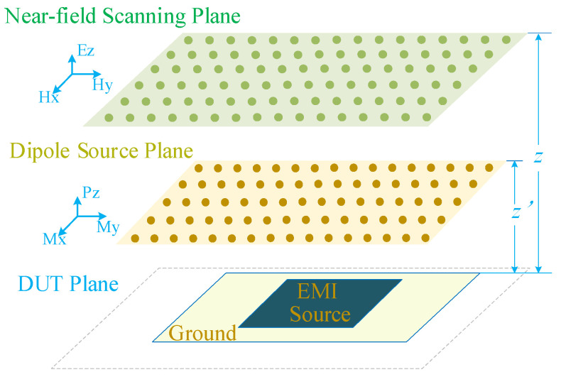 Figure 1
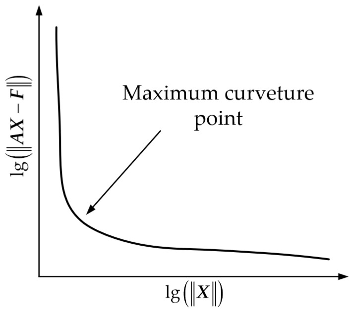 Figure 2
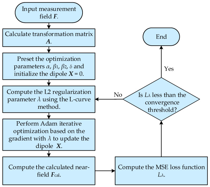 Figure 3
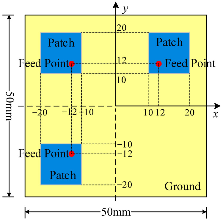 Figure 4
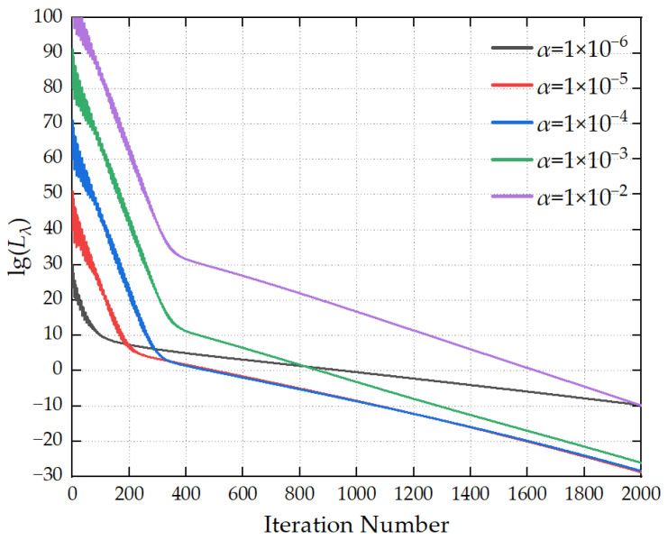 Figure 5
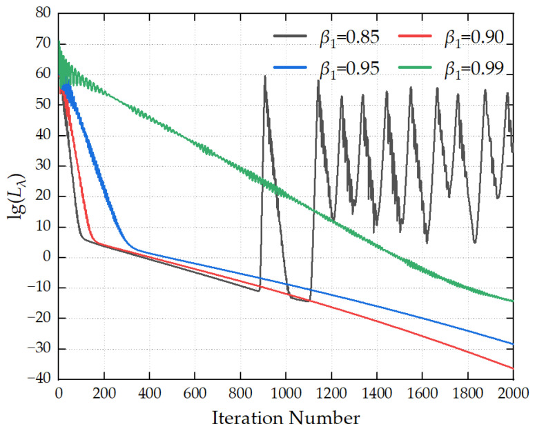 Figure 6
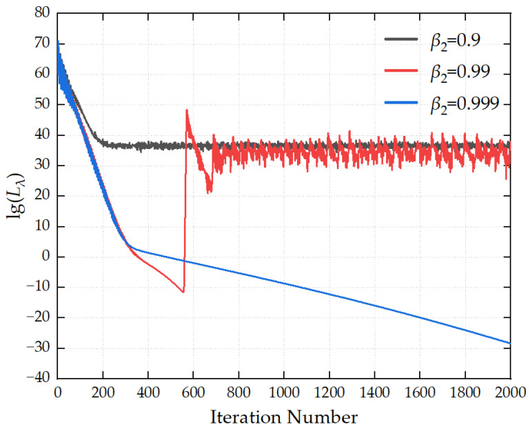 Figure 7
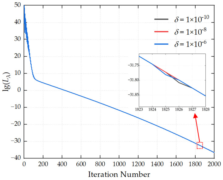 Figure 8
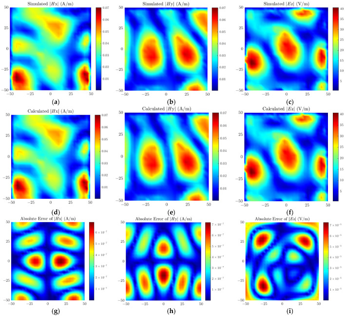 Figure 9
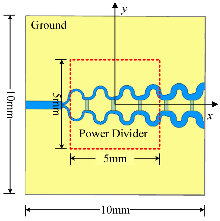 Figure 10
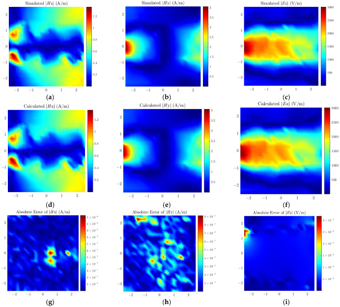 Figure 11
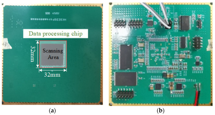 Figure 12
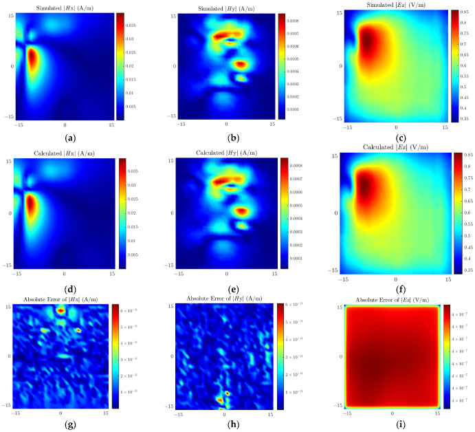 Figure 13
- —National Natural Science Foundation of China (NSFC)
Peer Reviews
No public reviews on file for this paper yet. If you reviewed it on a platform where reviews are public (OpenReview, ICLR, NeurIPS, ICML), you can paste yours below so the community can read it here.
Videos
No videos yet. Explain this paper in a talk, walkthrough, or lecture? Add one.
Taxonomy
TopicsElectromagnetic Compatibility and Measurements · Microwave Imaging and Scattering Analysis · Direction-of-Arrival Estimation Techniques
1. Introduction
With the rapid development of electronic devices, electronic components and their assembled electronic systems are evolving toward miniaturization, high density, high speed, and high frequency, and these trends inevitably aggravate electromagnetic interference (EMI) issues, posing significant challenges to electromagnetic compatibility (EMC) design [1,2]. Accurate EMI evaluation and identification of interference sources are essential for effective mitigation. In recent years, near-field scanning technology has been widely adopted in engineering practice as an efficient, flexible, and programmable approach for EMI source identification [3,4]. The process of acquiring near-field electromagnetic information of the device under test (DUT) using electric and magnetic field probes, followed by establishing an equivalent radiation source model, is referred to as source reconstruction. Due to commercial confidentiality and module packaging constraints, obtaining detailed physical dimensions and field distributions of noise sources has become increasingly difficult, making research related to source reconstruction particularly practically significant [5].
Using near-field test data, the equivalent source model of the DUT can be extracted, which mainly includes two core forms: the equivalent current model and the equivalent dipole model [6,7]. The construction of the equivalent current model is theoretically based on integral functions and Green’s functions [8]. The equivalent dipole model is established relying on the plane wave spectrum theory and the source reconstruction principle, and realizes the equivalent substitution of the actual radiation source through a set of infinitesimal dipoles with different types, amplitudes, phases and spatial position characteristics [9,10,11]. This model has important application value in scenarios such as near-field to far-field transformation, quantitative evaluation of near-field EMI, and diagnosis of electromagnetic emission problems. In recent years, the dipole model has also evolved from a single form to collections of multiple dipoles, distributed arrays, and spherical harmonic multipole expansion forms with high-order components, adapting to scenarios such as multi-source detection and complex target modeling [12,13,14].
Traditional equivalent dipole source reconstruction methods require the simultaneous acquisition of amplitude and phase information of different near-field components [15]. Due to limitations in measuring tangential electric-field components, obtaining complete phase data is complex and prone to error, motivating phaseless source reconstruction methods [16,17]. In the absence of phase information, the linear system of equations to be solved during the source reconstruction process is transformed into a nonlinear system of equations. Regularization methods based on the least squares method have been employed to solve the equivalent dipole model, integrating Tikhonov regularization and truncated singular value decomposition (TSVD) regularization [16]. However, these traditional methods are relatively sensitive to ill-conditioned transformation matrices, and the greater the condition number of the matrix, the poorer the solution accuracy and anti-noise performance. Additionally, to address this challenge, various global optimization algorithms—including differential evolution, genetic algorithms, and particle swarm optimization (PSO) algorithm—have been explored. Refs. [18,19] applied the differential dynamic evolution algorithm to solve the equivalent dipole model, and Ref. [20] further proposed the differential evolution algorithm; Ref. [21] utilized the genetic algorithm for equation solving; the PSO algorithm and quantum particle swarm optimization (QPSO) algorithm have also been adopted in source reconstruction studies [22,23,24]. These optimization algorithms also tend to fall into local optima and thus struggle to solve electromagnetic source reconstruction problems in complex multi-modal scenarios.
To address the aforementioned issues, this paper proposes a phaseless source reconstruction method combining the Adam optimization algorithm and L2 regularization. By means of the Adam optimization algorithm, the method avoids the direct inversion of ill-posed matrices. It not only improves the accuracy of near-field source reconstruction but also effectively avoids local optimal solutions. Meanwhile, the introduction of L2 regularization constrains the optimization process, further suppresses local optimality, and enhances the anti-noise performance of equivalent dipole solution. The fusion of the two ultimately achieves stable and accurate phaseless source reconstruction of complex near-field electromagnetic fields. It has a wide range of applications, covering EMI source localization in consumer electronics and near-field reconstruction of 5G high-frequency devices in the field of electronics and communications, as well as multi-source magnetic target detection and near-field coupling prediction of complex equipment in the field of general electromagnetic detection. This method can effectively solve the EMC challenges in related fields and possesses significant practical application value.
The structure of this paper is organized as follows: Section 2 elaborates on the proposed method in detail; Section 3 designs two sets of numerical experiments to verify the feasibility and accuracy of the method; Section 4 conducts an analysis based on the measured data of physical samples to complete the verification of the method’s practical effectiveness; finally, Section 5 summarizes the full text and draws the research conclusions.
2. Proposed Method
2.1. Equivalent Dipole Source
In the Cartesian coordinate system, six fundamental equivalent dipoles are defined: electric dipoles (P_x_, P_y_, P_z_) and magnetic dipoles (M_x_, M_y_, M_z_) [25]. This work employs M_x_, M_y_ and P_z_ dipoles to represent the actual EMI source, as illustrated in Figure 1. The core rationale for selecting M_x_, M_y_ and P_z_ is based on three key considerations.
First, the electromagnetic radiation of a printed circuit board (PCB) mainly consists of two components. One is the magnetic field radiation generated by the loop currents formed by different traces on the PCB, which can be equivalent to M_x_ and M_y_; the other is the electric field radiation induced by the potential difference between the PCB’s ground plane and metal structures such as traces, which can be equivalent to P_z_.
Second, developing high-performance tangential electric field probes that meet engineering requirements poses substantial challenges, resulting in high difficulty in measuring the tangential electric field in the near field [16]. Consequently, only the normal electric dipole P_z_ is selected among electric dipoles. Compared with the two tangential electric dipoles, the adoption of a single normal electric dipole can reduce the computational complexity of source reconstruction while improving the extraction efficiency of the equivalent source.
Third, most PCBs contain only a single ground plane. Owing to the image theory, the near-field radiation intensity of the dipoles M_x_, M_y_ and P_z_ is significantly higher than that of the dipoles P_x_, P_y_ and M_z_ [19].
In this paper, the normal near electric field and tangential near magnetic field are selected to verify the effectiveness of the proposed method using equivalent dipoles. Given the known equivalent dipole sources [16], the electromagnetic field distribution at any arbitrary point in space can be calculated as:
where the transformation matrix A serves as the mapping matrix between the electromagnetic field and the equivalent dipole sources, the matrix X denotes the equivalent dipole sources, and the matrix F represents the electromagnetic field distribution matrix at the observation points. The near-field distribution vector F includes the normal component of the electric field E_z_ and the tangential components of the magnetic field H_x_ and H_y_. The equivalent dipole vector X consists of the electric dipole P_z_ and the magnetic dipoles M_x_ and M_y_. The expanded form of (1) is given in Appendix A.
2.2. Adam Optimization Algorithm
A method for solving the electromagnetic inverse problem based on the Adam optimization algorithm is proposed to invert the source distribution from the measured electromagnetic field data. Its core logic resides in minimizing the mean square error (MSE) between the calculated field and the measured field through iterative optimization, thereby solving for the equivalent dipole X in (1). The specific implementation process comprises three steps.
The first step is initialization of data and variables. The equivalent dipole X is initialized as a zero vector, and the parameters of the Adam optimizer are configured. Meanwhile, the maximum number of iterations and convergence threshold are defined. The optimization parameters include the learning rate (α), first-order momentum coefficient (β1), second-order momentum coefficient (β2), and numerical stability term (δ). The learning rate, a core parameter controlling the step size of parameter updates, is defined as the scaling factor for parameter adjustments in each iteration. For nonlinear electromagnetic field inverse problems, a smaller learning rate can be selected to mitigate the impact of numerical instability. The first-order momentum coefficient is used to accumulate the exponential moving average (EMA) of gradients, reflecting the inertia of the parameter update direction. The second-order momentum coefficient accumulates the EMA of squared gradients, characterizing the scale properties of gradients. The numerical stability term is an extremely small positive value that ensures numerical stability while exerting a negligible influence on gradient scales, thus safeguarding the numerical accuracy of the optimization process. For nonlinear problems such as electromagnetic field inversion, appropriate parameter values enable efficient convergence to a reliable solution while ensuring numerical stability.
The second step is iterative optimization process. In each iteration, the calculated field is generated by the matrix multiplication of the transformation matrix A and the current equivalent dipole X. Subsequently, the residual r between the calculated field values and the measured field is calculated as follows:
where Fcal denotes the calculated field values, r represents the residual between the calculated field values and the measured field. It should be noted that the field values Fcal and F are only amplitude values without phase information.
Meanwhile, the MSE loss function L_MSE_ is calculated as follows:
where L_MSE_ is the MSE loss function. denotes the Euclidean norm of a matrix.
Further, the gradient of the loss function with respect to the equivalent source is derived by the transpose operation of the residual and the transformation matrix, which is computed as (4).
where g stands for the gradient of the loss function with respect to the equivalent source.
Finally, the equivalent dipole source X is iteratively updated using the momentum update rules of the Adam algorithm, as given by follows:
where m**t is the first-order momentum estimate at the t-th iteration, which serves to smooth the gradient update direction. v**t is the second-order momentum estimate at the t-th iteration, utilized for adaptively adjusting the learning rate. and are the bias correction terms for the first-order and second-order moments, respectively, designed to alleviate the bias issue of momentum estimates in the early stages of iteration. t denotes the number of iterations. ⊙ denotes the Hadamard product between matrices, also known as element-wise multiplication.
The third step is convergence criterion. The iteration is terminated when the difference in the loss function between adjacent iterations is less than the convergence threshold. Finally, the equivalent dipole X is obtained through inversion.
The Adam optimization algorithm stabilizes gradient fluctuations through momentum terms and avoids direct inversion of transformation matrix A. This effectively reduces the interference of ill-posed matrices with the solution results, improves the accuracy of the reconstruction field, and also effectively avoids local optimal solutions.
2.3. L2 Regularization
In electromagnetic field inversion problems, the condition number of the transformation matrix A is generally large, resulting in multiple sets of equivalent dipoles X that approximately satisfy the measured data in the solution space. Some of these solutions may contain physically unreasonable sharp fluctuations, leading to local optimization of the solution. L2 regularization imposes a penalty on the equivalent source X by introducing a regularization parameter λ: the value of λ directly determines the strength of the penalty term. By constraining the overall energy of the equivalent source X, L2 regularization confines the solution to a physically reasonable compact subspace, effectively suppressing numerical instability caused by ill-posedness. When λ is too small, the constraint is ineffective, causing overfitting; when λ is too large, excessive smoothing leads to underfitting. The solution becomes overly smoothed, losing details of the true source.
The integration of L2 regularization into the Adam optimization algorithm primarily involves three key stages: modifying the objective function, adjusting the gradient calculation, and influencing parameter updates.
First, the loss function changes from L_MSE_ to L_λ_, and the calculation formula is updated from (3) to (10). The newly added term acts as the regularization functional, where the regularization coefficient λ regulates its weight in the overall objective by scaling the value of the functional, thus guiding the optimization direction.
Second, the parameter update of the Adam algorithm relies on the gradient field of the objective function. After differentiating the regularized objective function, the total gradient function changes from g to , and the calculation formula is updated from (4) to (11). The newly added term λX is the regularization gradient, which imposes a constraint-guided effect on the solution.
Finally, the Adam algorithm achieves parameter update through the bias correction of the first-order momentum and second-order moment. The forms of its iterative formulas (5)–(9) remain unchanged; it only requires replacing the unregularized gradient g with the regularized gradient . The integration of regularization results in the update step size being subjected to stronger reverse correction, ultimately leading to the dynamic regularization of the solution.
In each iteration, we adopt the L-curve method to determine an appropriate value of λ [16]. We iterate over λ values within a predefined range and compute the corresponding and . Then, as illustrated in Figure 2, we plot the L-curve on a logarithmic scale, with as the abscissa and as the ordinate. The λ corresponding to the maximum curvature point is selected as the regularization parameter for the current iteration, thus achieving the dynamic adaptation of λ throughout the iteration process.
Mathematically, the penalty mechanism formed by introducing the L2 regularization parameter λ not only enhances the anti-noise performance of electromagnetic field inversion but also effectively prevents the optimization process from falling into local optima. By integrating L2 regularization with the Adam optimizer, the proposed method not only achieves high accuracy and strong anti-noise performance but also effectively avoids convergence to local minima. The flow chart of the proposed method is shown in Figure 3.
The computational complexity of the proposed method is mainly determined by two key factors: the number of iterations and the dimension of optimization variables. The algorithm achieves the required accuracy after a fixed number of iterations, which is a constant value in our method. The dimension of optimization variables is only related to the number of equivalent dipoles and their amplitudes, denoted as N. The core computation in each iteration involves matrix operations and gradient updates based on the Adam optimization algorithm, resulting in a time complexity of O(K × N^2^), where K represents the number of iterations. In terms of space complexity, it is dominated by the storage of dipole amplitudes, gradient information, and intermediate calculation results, with a space complexity of O(N). Regarding scalability, the proposed method exhibits excellent adaptability: when the number of dipoles (N) increases or the number of measurement points expands to adapt to more complex near-field scenarios, the time complexity grows moderately with N^2^, which is fully manageable with current computing resources. Meanwhile, the fixed number of iterations avoids excessive complexity growth caused by additional iterations, ensuring that the method can be scaled to practical large-scale near-field source reconstruction tasks.
3. Simulation Examples and Validation
In this section, the effectiveness of the proposed method is verified through multiple repeated simulations and calculations by combining two simulation-based numerical examples. The proposed method is implemented on a computer equipped with an Intel Xeon Gold 6146 3.20 GHz CPU and 128 GB RAM.
3.1. Application in Patch Antenna
The first simulation example consists of three 10 mm × 10 mm patch antennas, with the model illustrated in Figure 4. The dielectric substrate is duroid 5880 with a thickness of 3.2 mm, and the ground plane measures 50 mm × 50 mm. The positions of the three feeding points are (12 mm, 12 mm), (−12 mm, 12 mm) and (−12 mm, −12 mm), respectively, and the operating frequency is set to 4 GHz. The near-field observation plane is a 50 mm × 50 mm area located 4 mm directly above the patch antennas, while the dipole plane is deployed in the same area at a height of 1.5 mm. The number of observation points is 26 × 26 with a spacing of 4 mm between adjacent points, and the number of dipoles is 21 × 21 with an interval of 5 mm between each dipole.
3.1.1. Parameter Analysis
The maximum number of iterations is set to 2000, and the convergence threshold is configured as 1 × 10^−8^. The optimization hyperparameters are preset as follows: the learning rate α is 1 × 10^−5^, the first-order momentum coefficient β1 is 0.90, the second-order momentum coefficient β2 is 0.999, and the numerical stability term δ is 1 × 10^−8^. The optimal values of the aforementioned hyperparameters are determined by comparing the iterative convergence curves generated under different parameter configurations.
Figure 5 illustrates the variation in the loss function with the number of iterations under different α values. When α is excessively large, the initial loss function value remains high, resulting in a still elevated loss function value at the end of iterations. When α is too small, the loss function converges slowly, leading to low iteration efficiency. When α is set to a moderate value, a balance is achieved between the initial loss function value and the convergence speed. It is recommended that the value range of α be set to 1 × 10^−5^∼1 × 10^−4^.
Figure 6 illustrates the influence of different first-order momentum decay coefficients β1 on the convergence process of the loss function. When β1 is excessively large, the loss curve tends to exhibit severe oscillations, which results in the non-convergence of the loss function. When β1 is too small, the loss function decreases at an overly slow rate, leading to low solution accuracy. When β1 is assigned a moderate value, a favorable balance is achieved between convergence speed and convergence stability. It is recommended that the value of β1 be set to 0.9.
Figure 7 illustrates the influence of different second-order momentum decay coefficients β2 on the convergence process of the loss function. When β2 takes a relatively large value, the loss curve declines rapidly in the early stage of iterations and can achieve continuous convergence. When β2 is too small, the loss function tends to fall into oscillations and fails to converge. It is recommended that the value of β2 be set to 0.999.
Figure 8 demonstrates the influence of different numerical stability parameters δ on the convergence process of the loss function. The three curves in the figure almost completely overlap, and there are no significant differences in the initial values, decline rates, and final convergence accuracy of the loss function. As long as δ lies within a reasonable small value range, it will not exert a noticeable impact on the convergence performance. It is recommended that the value of δ be set to 1 × 10^−8^.
The amplitude values of the simulated field for the patch antenna model range from 1 × 10^−2^ to 40. From the convergence curves obtained under the influence of different optimization parameters mentioned above, it can be concluded that the loss function of the proposed method has already become very small when the number of iterations reaches 2000. At this point, the loss function is close to 1 × 10^−4^, which is 2 to 3 orders of magnitude smaller than the simulated field amplitude values, indicating that the source reconstruction accuracy is quite high within the limited number of iterations. The convergence threshold is defined as the difference between the loss functions of two adjacent iterations, which is generally 2 to 4 orders of magnitude smaller than the loss function itself. Therefore, the number of iterations is set to 2000 and the convergence threshold is set to 1 × 10^−8^.
In summary, to achieve high-precision source reconstruction, it is recommended that the number of iterations be set to 2000, the convergence threshold to 1 × 10^−8^, the learning rate to 1 × 10^−5^, the first-order momentum coefficient β1 = 0.9, the second-order momentum coefficient β2 = 0.999, and the numerical stability term δ = 1 × 10^−8^.
3.1.2. Global Optimization
The proposed method features the core characteristic of global optimization. When addressing multimodal optimization problems, local optimization algorithms are often constrained by local information in the solution space and prone to trapping in local optimal solutions, making it difficult to achieve globally optimal solutions. The antenna model adopted in this study has a radiated field with distinct multimodal distribution characteristics, which can serve as a typical test case for verifying algorithm performance and effectively demonstrate the feasibility and superiority of the proposed method.
Figure 9 presents the simulated field, calculated reconstructed field, and the distribution of absolute errors between the two for the antenna model, where the absolute error is defined as the amplitude difference between the simulated field and the calculated field. As can be seen from Figure 9, the amplitude of the absolute error is five orders of magnitude lower than that of the simulated field, which fully indicates that the source reconstruction accuracy of the proposed method reaches a high level. Meanwhile, the errors corresponding to each peak region in the field distribution are maintained within an extremely small range, further verifying the excellent global optimization performance of the proposed method, which holds broad prospects for engineering applications.
3.1.3. Accuracy
To address the issue of overall error distortion caused by the amplification of relative error in weak signals, a weighted relative error (εwr) is defined as (12) to quantitatively analyze the effectiveness of the proposed method. This relative error weights the error at each measurement point using the field value of that point, achieving weighted enhancement of strong signals and weighted reduction in weak signals. It can objectively reflect the reconstruction accuracy of the effective source region and is more referenceable in practical measurements.
where Fsim denotes the measured field from the true source or simulated source, and Fcal represents the reconstructed field from the equivalent dipole source, both of which consist of three electromagnetic field components. (i, j) is the two-dimensional grid row and column index of the measurement point. ε is a tiny constant that provides robust correction for weak signals and noise points. The range of εwr is (0, 100%); the closer its value is to 0, the better the performance of the reconstructed field.
To demonstrate the accuracy of the proposed method, a comparison is conducted with the Adam optimization algorithm with regularization and a traditional least squares method. The traditional method selected is the phaseless source reconstruction method combining Tikhonov regularization and TSVD regularization proposed in [16]. By establishing dipoles at different plane heights to generate reconstructed fields, comparisons of weighted relative error εwr under various conditions are obtained, as presented in Table 1. The weighted relative error of the proposed method is significantly smaller than that of the traditional method. Meanwhile, it can be observed that when the height of the equivalent dipoles is set within the range of 1.5 mm to 3 mm, the source reconstruction error is minimal.
3.1.4. Anti-Noise Performance
The correlation coefficient ρ is defined as (13), which serves to quantitatively evaluate the similarity between the calculated field and the simulated field. The value range of ρ is (−1, 1); the closer this value is to 1, the better the source reconstruction performance.
where Cov denotes the covariance operation of matrices, and Var denotes the variance operation of matrices.
Near-field measurements are susceptible to external noise interference, where the measured data are a mixture of the true field values and noise. Therefore, the research on source reconstruction methods must take anti-noise performance into account. The simulated field is regarded as a pure noise-free reference, and the anti-noise performance of source reconstruction methods is compared between this reference and the simulated field injected with white Gaussian noise of varying intensities. White Gaussian noise is commonly encountered in engineering; the noise intensity is set to be correlated with the amplitude of the simulated field, calculated as follows:
where Fpure is the pure magnetic field matrix, N**F is the generated white Gaussian noise matrix, and is a random matrix following a normal distribution. The three matrices are of the same dimension. L_n_ is the noise level coefficient, which is used to adjust the relative magnitude of the noise. Noise level coefficients of 2%, 5%, 10%, 20%, 30%, and 40% are selected to compare the anti-noise performance of different methods.
White Gaussian noise with different intensities is injected into the pure simulated field; source reconstruction is performed separately to obtain the calculated field. All similarity indices are calculated as the similarity between the calculated field and the pure simulated field under different noise levels. By comparing the attenuation amplitude of similarity under different noise levels, the anti-noise performance of the proposed source reconstruction method is quantitatively evaluated.
The comparison results of source reconstruction similarity under different noise levels are presented in Table 2. As can be seen from Table 2, at noise levels below 10%, the anti-noise performance of the proposed method and the basic Adam optimization method is significantly superior to that of the traditional method, with the similarity decreasing by less than 2%. Meanwhile, as the noise level increases, the anti-noise performance of the proposed method becomes increasingly superior to that of the basic Adam optimization method. By introducing a regularization coefficient into Adam optimization, the sensitivity of source reconstruction to noise interference is effectively suppressed. L2 regularization can improve the anti-noise performance of source reconstruction methods and thus can be effectively applied to phase-free source reconstruction in electromagnetic near-field measurements.
3.2. Simulation of Power Divider
The proposed method is verified through a simulated power divider, as illustrated in Figure 10. The PCB dimensions are 10 mm × 10 mm, and the dielectric substrate is FR4 with a thickness of 3 mm. The three terminal impedances of the power divider are all set to 50 Ω, and the input power of the unbalanced port is set to 1 VA. The selected region is a 5 mm × 5 mm area 1 mm above the transmission line, where the near-field data is collected. The number of observation points is 21 × 21, with a spacing of 0.25 mm between adjacent observation points. The dipole height is set to 0.5 mm; the number of dipoles is 19 × 19, and the spacing between adjacent dipoles is 0.26 mm. Figure 11 presents the simulated field, calculated field, and the distribution of absolute errors between the two for the power divider model. Similarly, Table 3 lists the weighted relative error for both methods, showing that the proposed method outperforms the traditional method in accuracy.
4. Measurement Examples and Validation
In this section, physical verification of the proposed method is conducted. A test board of a data processing chip is selected as the DUT, and the front and back sides of the main board are illustrated in Figure 12. The DUT is measured to verify the effectiveness and accuracy of the proposed method.
The test procedure for electromagnetic near-field radiation emission is as follows: The DUT is powered by a DC power supply and excited by a signal generator. The near-field probe is vertically placed 1 mm above the DUT and moved point-by-point in the two-dimensional plane above the DUT via a robotic arm. The near-field probe converts the field signal into an electrical signal, which is read and recorded by a spectrum analyzer connected through a coaxial cable. Both the electric field probe and magnetic field probe used in the measurement were pre-calibrated [26,27].
The near-field scanning area is a 32 mm × 32 mm region 1 mm directly above the chip. The number of scanning points is 33 × 33, with a spacing of 1 mm between adjacent scanning points. The dipole source plane is set at a height of 0.5 mm; the number of dipoles is set to 25 × 25, and the spacing between adjacent dipoles is 1.33 mm. The scanned near-field and the near-field generated by the equivalent dipole sources are shown in Figure 13. The comparison between the proposed method and the traditional method is presented in Table 4, demonstrating that the dipole model of the proposed method has higher accuracy than that of the traditional method.
5. Conclusions
This study proposes a phaseless source reconstruction method integrating the Adam optimization algorithm with L2 regularization, which effectively overcomes the limitations of traditional methods and other optimization algorithms in solving near-field inverse problems. Verified quantitatively through numerical simulations and physical measurements, the method exhibits excellent performance in reconstruction accuracy, anti-noise capability, and global optimization performance. In terms of reconstruction accuracy, the weighted relative error εwr of the proposed method can be as low as 0.0001%, and the absolute error is five orders of magnitude smaller than the amplitude of the measured field. Regarding anti-noise performance, when the noise level coefficient does not exceed 10%, the decrease in the correlation coefficient ρ is less than 2%, demonstrating extremely strong anti-noise performance. Additionally, the method has broader applicability compared with other optimization methods—even in complex scenarios with multimodal near-field distributions, the reconstruction error in each peak region remains minimal, enabling accurate field reconstruction.
However, the parameter selection of the Adam optimization algorithm is crucial; improper configuration may lead to failure to converge during iterations. Future research can integrate big data and neural networks to realize automatic optimal parameter selection without manual debugging, further enhancing the engineering practicality and efficiency of the method.
The dipole source reconstruction method proposed in this study, with its excellent anti-noise performance and superior reconstruction accuracy, is suitable for moderate-complexity near-field tasks such as EMI source localization in consumer electronics and the near-field reconstruction of 5G devices. It should be noted, however, that the proposed method does not incorporate higher-order momentum sources, which limits its broader applicability. Spherical harmonic expansion can decompose complex electromagnetic sources into multipole components including dipoles and quadrupoles. In the future, our method can draw on multi-source modeling strategies to improve the existing Adam optimization algorithm framework, enabling it to simultaneously optimize the amplitudes of both dipole and quadrupole components, thereby developing a near-field source reconstruction method applicable to more complex scenarios such as aerospace, automotive, and marine engineering fields.
The reference list from the paper itself. Each links out to its DOI / PubMed record.
- 1Wu I. Shiota S. Matsumoto Y. Gotoh K. Application of Reverberation Chamber for Radiated Emission Testing for Wireless Protection Toward Full-Scale Deployment of 5G System—Advantages and Challenges IEEE Access 202311782737828410.1109/ACCESS.2023.3298368 · doi ↗
- 2Luo R. He Z. Wang L. Broadband Low-Cost Normal Magnetic Field Probe for PCB Near-Field Measurement Sensors 202525387410.3390/s 2513387440648135 PMC 12251827 · doi ↗ · pubmed ↗
- 3Obermaier M. Lange J. Deckert T. Vanden Bossche M. Plettemeier D. Compact Multi-Probe Planar Near Field Antenna Measurement System Proceedings of the 2025 55th European Microwave Conference (Eu MC)Utrecht, The Netherlands 23–25 September 2025
- 4Zhao Y. Lu R.P. Song Z.Q. Mou X.Y. Hu Y.W. Du G.H. EMC Near-field Scanning System with Fast Scanning Method Proceedings of the 2024 Photonics & Electromagnetics Research Symposium (PIERS)Chengdu, China 21–25 April 2024
- 5Qin J. Wang W. Wu Y. Zeng Q. Liu Y. Integrated Circuit Radiation Source Reconstruction Method Based on Deep Neural Network Proceedings of the 2025 IEEE International Workshop on Electromagnetics: Applications and Student Innovation Competition (i WEM)Hong Kong, China 4–6 August 2025
- 6Huang X.T. Liu Q.F. Chen H. Li Y.M. Huang C. Zhu X.G. Zhang H.Q. Yin W.-Y. A New Hybrid Equivalent Modeling Method of Low-Frequency Radiation Source Based on GS and JADE Algorithms and Phaseless Near-Field Data IEEE Trans. Electromagn. Compat.20246691792710.1109/TEMC.2024.3359259 · doi ↗
- 7Zhang S.-Q. Wu Y.-L. Ma Z. Hu C.-H. Jian X. Shang H.-Q. Liu S.-H. Distributed Equivalent Circuit Model of Dipole Based on Radiation Characteristics IEEE Antennas Wirel. Propag. Lett.20232286887210.1109/LAWP.2022.3227218 · doi ↗
- 8Gao T.F. Yan Z.W. Hu K.K. Zhao F.Y. Zhao X.Y. Ge J.H. A Planar Sheet-Type Composite Electric and Magnetic Near-Field Probe IEEE Antennas Wirel. Propag. Lett.20251510.1109/LAWP.2025.3644401 · doi ↗