On the Variability of the Barometric Effect and Its Relation to Cosmic-Ray Neutron Sensing
Patrick Davies, Roland Baatz, Paul Schattan, Emmanuel Quansah, Leonard Kofitse Amekudzi, Heye Reemt Bogena

TL;DR
This study shows that the barometric coefficient varies by location and sensor type, requiring site-specific corrections for accurate soil moisture measurements using cosmic-ray neutron sensing.
Contribution
The study introduces a method for deriving site- and sensor-specific barometric coefficients to improve soil moisture estimation.
Findings
Barometric coefficients (β) vary spatially and temporally, with values differing between CRNS and neutron monitor stations.
Empirical methods for estimating β show stronger agreement with each other than with analytical approaches.
Sensor type and elevation significantly influence β values, while soil moisture and humidity have negligible effects.
Abstract
Accurate estimation of the barometric coefficient (β) is important for correcting pressure effects in soil moisture data from cosmic-ray neutron sensing (CRNS) due to the barometric effect. To evaluate estimation strategies for β, we compared analytical and empirical approaches using 71 CRNS and 46 neutron monitor (NM) stations across the United States, Europe, and globally. Our results show spatio-temporal variation in the barometric effect, with β ranging from 0.66 to 0.82 %hPa for NM and from 0.63 to 0.80 %hPa for CRNS. These coefficients exhibit higher variability than previously published semi-analytical models. In addition, we found that the analytically determined β values were systematically lower compared with empirical estimates, with stronger agreement between the two empirical methods (r≈0.67) than between empirical and analytical approaches. Furthermore, NM stations…
Click any figure to enlarge with its caption.
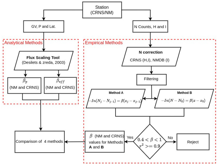 Figure 1
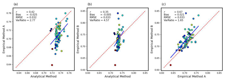 Figure 2
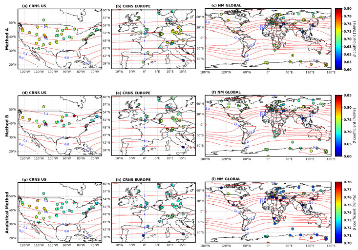 Figure 3
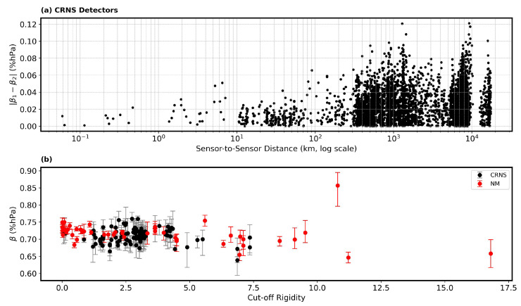 Figure 4
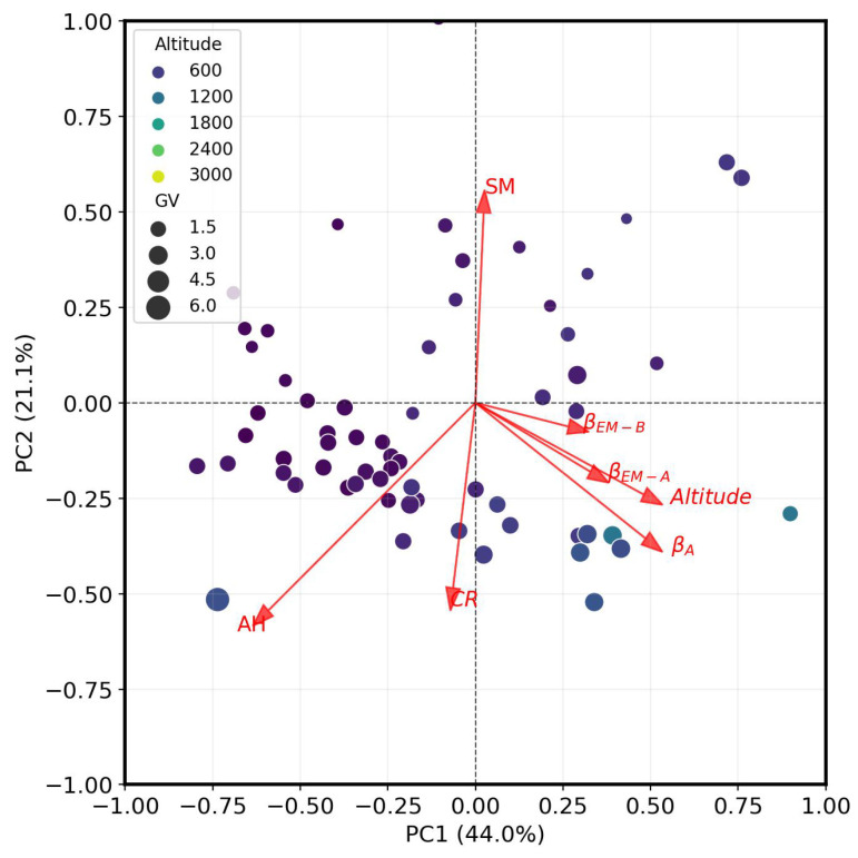 Figure 5
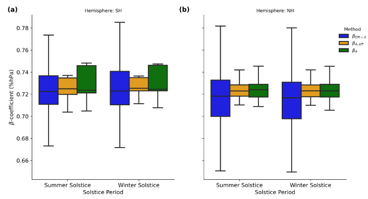 Figure 6
 Figure 7
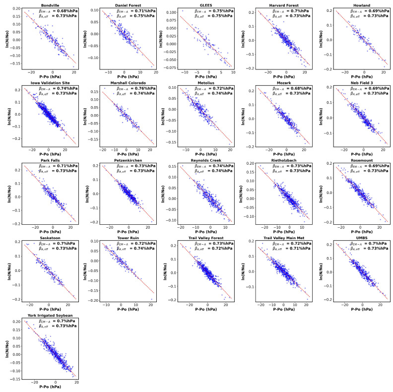 Figure 8
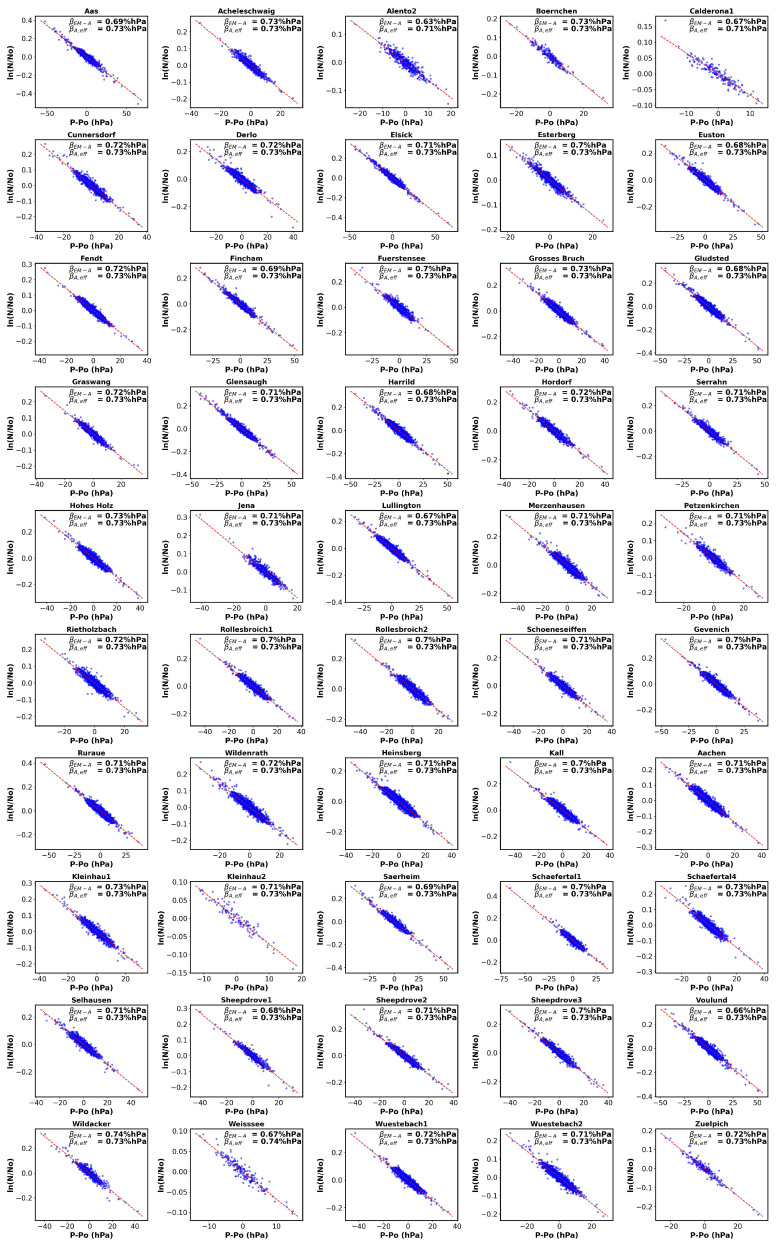 Figure 9
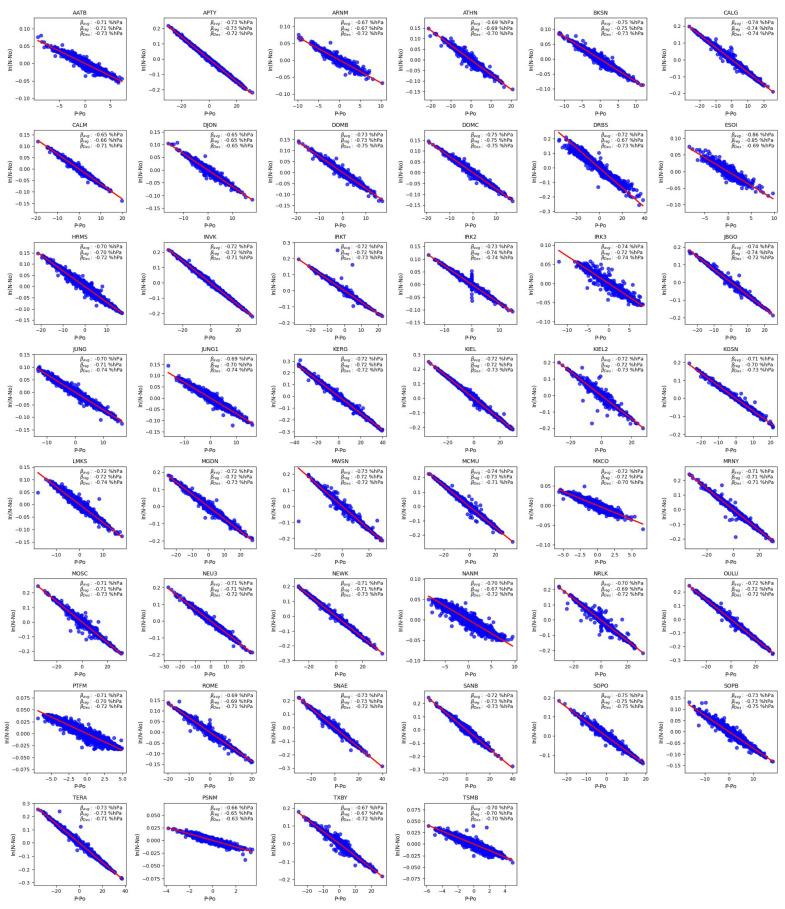 Figure 10
- —Federal Ministry of Education and Research (BMBF)
- —Austrian Science Fund
Peer Reviews
No public reviews on file for this paper yet. If you reviewed it on a platform where reviews are public (OpenReview, ICLR, NeurIPS, ICML), you can paste yours below so the community can read it here.
Videos
No videos yet. Explain this paper in a talk, walkthrough, or lecture? Add one.
Taxonomy
TopicsSoil Moisture and Remote Sensing · Urban Heat Island Mitigation · Ionosphere and magnetosphere dynamics
1. Introduction
The cosmic-ray neutron sensing (CRNS) method [1,2] effectively estimates soil water content (SWC) based on the inverse relationship between cosmic-ray neutron intensity near the land surface and hydrogen present in soil water. The method is commonly used at the field scale [3] and can also be useful at the continental scale by integrating CRNS networks [4].
Cosmic-ray neutrons are secondary particles produced by inelastic collisions of high-energy primary particles from outer space with Earth’s atmospheric nuclei [5] which are then moderated by elastic collisions with hydrogen nuclei [6]. Inelastic collision processes lead to the attenuation of the nucleon cascade, and their effectiveness depends on the mass thickness of the atmosphere, which is typically represented by the barometric pressure. Since the barometric pressure of the atmosphere fluctuates over time with changing weather conditions, substantial temporal fluctuations occur in the neutron count rate of a CRNS detector. Consequently, the correction for the barometric effect is one of the most important data corrections for CRNS [2], for which reason CRNS sensors are always equipped with a pressure sensor [7]. In addition, fluctuations in the solar and geomagnetic fields modulate the amount of high-energy cosmic rays penetrating the atmosphere, which leads to further changes in the intensity of cosmic-ray neutrons [8,9]. Temporal variations in cosmic-ray neutrons due to these influences are detected with neutron monitors (NMs) [10], which are sensitive to high-energy secondary neutrons but insensitive to local environmental factors such as SWC. Therefore, NM data are typically used to correct CRNS raw data from fluctuations in incoming neutrons [11].
Although the general dependence of barometric coefficients on geomagnetic latitude and altitude has been known for some time [12], in CRNS applications, as an approximation, the coefficient is often assumed to be constant in time and space. For example, a coefficient of 0.76 % hPa suggested by [13] was generally applied across the COSMOS-Europe network [4]. Notably, the range of estimates for COSMOS-Europe sites in a recent data-driven study [14] was considerably broader, spanning 0.52 to 0.78 %hPa (with a mean of 0.71 %hPa and a median of 0.73 %hPa), than the commonly utilized reference value of 0.76 %hPa. Studies have shown that the barometric coefficient is a complex variable that depends on factors such as geographical latitude, altitude, type and energy of incoming primary particles [14,15,16], and solar activity [6,17]. In addition, the barometric coefficient depends on the energy sensitivity of the detector [18], as the nucleon energy spectrum shifts towards lower energies as the barometric coefficients decrease [19]. Therefore, since the energy range covered by NMs (∼0.5 to 100 GV; [18]) differs strongly from CRNS (∼0.1 eV to 1 MeV; [20]), it can be assumed that the determined with neutron count rates observed by CRNS detectors and NMs are also different. In the past, analytical relationships of have been mainly derived from selected neutron monitor locations across a wide range of geomagnetic cut-off rigidities but with varying altitudes [13,16,21,22,23]. Further relations were established using data from ship-based latitude surveys [24,25]. In addition to solely minimizing the correlation between incident radiation and atmospheric pressure [26], some studies also included the normalization of the data with a reference NM to remove effects of variations in the incoming comsic-ray flux [16,27]. A study incorporating different neutron detection energies [19] found that the attenuation length (i.e., the inverse of ) ranged from 128 to 142 gcm^−2^ at altitudes between sea level and 5000 m when using NM data, whereas attenuation lengths derived from thermal neutron data are somewhat higher, ranging from 134 to 155 gcm^−2^ at similar altitudes. For Europe, the difference in is small when using a single analytical function [4]. Still, the results for a location at a cut-off rigidity (CR) of 4.5 GV would vary from an attenuation length of 132 to 142 gcm^−2^ when using different analytical equations [16,24,25].
Therefore, this study proposes a site- and energy-specific estimation of using local CRNS data instead of a global fit based on NM data to obtain more suitable values for in the effective energy range of CRNS sensors. Additionally, we compare the values of obtained using our new method with those determined by three empirical and analytical methods. This study is the first to jointly determine coefficients for numerous CRNS (71 stations in Europe and the USA) and NM (46 globally) stations and analyze their spatio-temporal variability.
2. Materials and Methods
Our methodological framework is designed to determine coefficients from hourly, long-term records of cosmic-ray intensity measured with neutron detectors. The approach combines two analytical methods and two empirical methods (labeled A and B), allowing for both theoretical derivation and data-driven estimation. For the empirical component, we draw upon extensive observational datasets:
- Cosmic-ray neutron sensing (CRNS) networks comprising 71 stations across the United States [2] and Europe [4].
- Neutron Monitor Database (NMDB), which provides data from 46 stations worldwide (https://www.nmdb.eu/).
The NMDB archive spans 1958–2023 and covers sites with geomagnetic cut-off rigidities between 0 and 16.8 GeV, while the CRNS stations fall within the narrower range of 1–7.5 GeV. Together, these datasets provide a robust basis for performing evaluation across diverse spatial and temporal conditions.
2.1. Data Processing and Quality Control
The data-driven empirical methods (A and B) were applied following standard CRNS corrections (humidity and incoming neutron intensity) and the filtering of neutron count data from CRNS and NM stations to address known environmental influences and to ensure data comparability across sites. The quality criteria included removing data with unrealistic temporal behavior due to sensor malfunctioning, as well as values out of the physical ranges for air humidity, air pressure, and neutron flux. Additionally, months with fewer than 18 days of daily neutron observations were considered insufficiently representative and were excluded from the analysis. The filtered data were then corrected for fluctuations in the incoming cosmic-ray neutron intensity, which can introduce temporal noise unrelated to local atmospheric conditions. We applied the correction approach developed by [11], ensuring that both the NM and CRNS datasets reflected consistent background intensity levels.
For CRNS stations, an additional correction was applied to account for atmospheric humidity [28], which attenuates neutron flux and can bias measurements if left unadjusted. This humidity correction was implemented using site-specific humidity records and established calibration procedures. Following these corrections, the relationship (barometric coefficient) between neutron counts and atmospheric pressure was estimated for each station using the two empirical methods (A and B) and the analytical approach by [19]. Figure 1 summarizes the overall workflow, including input variables, correction steps, and the branching into analytical scaling and empirical regression approaches to estimating .
2.2. Methods
Data-Driven Approaches to Barometric Coefficient Estimation
The influence of atmospheric pressure on the flux of cosmic-ray neutrons N (i.e., the barometric effect) can be corrected using the following Equation (1) described in [29,30].
where is the reference atmospheric pressure, P is the atmospheric pressure at the time of observation in hPa, is the corrected neutron count rate, and is the barometric coefficient in %hPa. By integrating Equation (1), we obtain an Equation (2), which allow us to infer the coefficient as the slope of a linear regression:
The derived equation was applied in previous studies to the NM dataset to estimate the coefficient [27].
Building on the pressure-based formulation in Equation (2), we developed two empirical methods for estimating directly from corrected neutron count data. This equation expresses the logarithmic relationship between the pressure-adjusted neutron flux and deviations from a reference pressure, providing a physically grounded basis for regression-based estimation. By adapting this structure to station-level time series, we formulated two empirical variants (Methods A and B) that differ in how they define reference states and temporal increments. The atmospheric air pressure (P) was converted into atmospheric depth x (gcm^−2^) based on gravity (g) using Equation (3) as described in [11] for the two empirical approaches.
Method A is based on Equation (2) to estimate daily from corrected neutron count rates, as shown in Equation (4):
where and are the corrected neutron count rates and atmospheric depths x in gcm^−2^ on day j and on the previous day, , respectively. To minimize the impact of changes in ambient water, neutron counts that deviated by more than 10% from the previous and subsequent readings were excluded. Method A is consequently less susceptible to changes in soil moisture and is therefore particularly suitable for ground-based CRNS data. Empirical method B adopts the approach proposed by [23,27] to estimate , as shown in Equation (5):
where and are the average observations of hourly neutron counts and atmospheric depth. Note that for both empirical methods, monthly were estimated using CRNS and NM data, as suggested by [23]. To ensure high accuracy of the estimated values, only regressions with and between 0.004 and 0.02 %hPa are considered valid (see Figure A3 and Figure A4 for method A’s regression). The resulting monthly estimates are then averaged to obtain a mean and standard deviation ( ) for the respective CRNS and NM stations. This approach, based on a large number of individual monthly values, results in more robust estimates, reducing the statistical noise expected, e.g., from changes in ambient moisture conditions.
2.3. Analytical Methods
The analytical method developed by [19] has become the predominant approach for determining in the past decade. This approach, based on previous studies, e.g., [12,31], determines the barometric coefficient at a certain atmospheric depth ( ) by utilizing the theoretical relation between the coefficient and its key affecting elements, namely, cut-off rigidity and altitude ([12]):
To further estimate the effective barometric coefficient ( ) between two atmospheric depths and , Equation (7) is used as follows:
where and are dependent on the location (cut-off rigidity ( ) and latitude (Lat)) and the atmospheric depth x in gcm^−2^, , , and . Each site’s atmospheric depth (x) is derived from pressure information using Equation (3). This analytical approach is also available online as a ‘Flux scaling tool’ (https://crnslab.org), which provides yearly estimates of based on longitude, altitude, and latitude. In this study, we applied the analytical framework described in [19] using site-specific monthly pressure data rather than annual averages. Monthly pressure measurements were converted into altitude using Equation (7), and was calculated for each month following the same theoretical framework. This approach allows us to capture temporal variability associated with seasonal pressure patterns while maintaining consistency with the established analytical method.
2.4. Principal Component Analysis (PCA)
Principal Component Analysis was applied to identify orthogonal modes of variability in the relationship between the CRNS coefficient and environmental covariates. For each site , we obtained method-specific estimates of parameter : analytical ( ), empirical A ( ), and empirical B ( ). In addition, each site was characterized by environmental and geophysical variables, including soil moisture ( ), atmospheric humidity ( ), and geomagnetic cut-off rigidity ( ). These values were assembled into a data matrix:
The variables were standardized to ensure comparability across scales. Principal Component Analysis was then applied to the standardized matrix to reduce dimensionality and identify dominant modes of variability. The covariance matrix was computed as
where X is the standardized data matrix. Eigendecomposition of S yielded orthogonal loading vectors and associated eigenvalues, which define the principal components. Site scores were obtained by projecting the standardized data onto the loading vectors. The proportion of variance explained by each component was calculated as
where is the eigenvalue of component k. For visualization, the first two principal components were retained, and a biplot was constructed. In this representation, site scores are plotted in the PC1–PC2 space, while variable loadings are displayed as vectors scaled by the square root of their corresponding eigenvalues. This allows for the simultaneous visualization of site clustering and the relative contributions of method-specific estimates and geophysical variables.
3. Results
The agreement between the analytical and empirical approaches for estimating is shown in Figure 2, with scatter plots (Figure 2a–c) comparing the CRNS-estimated values derived from the analytical method (the proposed method; ) with those from two empirical methods (A and B), as well as the comparison between the two empirical methods. Figure 2a, the comparison between the analytical method ( ) and empirical method A ( ), reveals a moderate positive correlation ( ), and a variability ratio of 2.77, indicating some agreement with analytical but also noticeable scatter, particularly at lower values. A slightly weaker correlation (r = 0.35) is observed between the analytical method and empirical method B (see Figure 2b), with RMSE = 0.033, and a higher variability ratio of 4.57, reflecting greater spread and overestimation of variance despite its lower bias. In contrast, Figure 2c demonstrates a stronger relationship between the two empirical methods ( , , and variability ratio = 1.65), suggesting greater consistency between empirical approaches than between empirical and analytical methods. Overall, both empirical methods show limited agreement with the analytical reference, but method A performs slightly better by combining lower RMSE, stronger correlation, and more moderate variance. Given that aligns more closely with the analytical method and provides more stable estimates than method B, we present results from empirical method A to provide a balanced and consistent perspective on .
3.1. Estimated Barometric Coefficients Using Empirical and Analytical Methods
Figure 3 presents the spatial distribution of monthly averaged coefficients derived from three methods (analytical and empirical methods A and B) over a period for CRNS stations in the US and Europe, as well as NM stations globally. The red contour lines represent geomagnetic cut-off rigidity values, providing context for the spatial variability in atmospheric pressure corrections. The results from empirical method A ( ) reveal the average of monthly coefficients ranging from 0.60 to 0.80 across all networks, with the majority of CRNS stations clustering between 0.65 and 0.75. In the US, approximately 95% of stations exhibit values within this range, while European stations (≈96%) show similar values. The global NM network demonstrates comparable ranges, though out of 47 NM stations, 4 stations recorded an average of monthly %hPa (see Figure 3a–c).
The average estimates derived from CRNS data were %hPa and %hPa for stations in the US and Europe, respectively. Analysis of global NM data gave an average of (Table 1). Method B ( ) shows a similar range but extends the upper limit to 0.85 %hPa compared with method A. US CRNS stations show the most pronounced increase for some locations, exceeding 0.75, particularly in the northern part. European stations maintain their spatial patterns but with enhanced magnitude, while the global NM distribution exhibits marginal shifts toward higher values in the Northern Hemisphere mid-latitudes. yields comparable average values across all networks, with %hPa for US CRNS, %hPa for Europe CRNS, and for the global NM network (Table 1).
The analytical method (Figure 3g–i) produced a more constrained range of averaged monthly estimated (0.70–0.75 %hPa) compared with empirical methods A and B. Both US and Europe CRNS stations showed less variation in the averaged monthly between and %hPa. European stations were clustered tightly around 0.73–0.75, and the global NM network showed a similarly reduced variability pattern. All three methods showed a pronounced longitudinal decrease from the western part of the US (120°W) to the east (70°W) (see Figure 3a,d,g), although the range of the analytical variability is smaller than that of the empirical methods. Strong regional contrasts are observed for Europe, with higher empirical barometric coefficient ( and ) values in the continental interior (0.68–0.76 %hPa at 50°N–54°N) compared with the analytical method. At the global scale, a clear indication of an inverse relation between the cut-off rigidity and the estimated coefficient was observed using the NM (see Figure 3c,f,i). Overall, values exhibit relatively consistent ranges across methods and regions, with only minor differences between empirical and analytical estimates. The values for CRNS (in both the US and EU regions) and for NM sensors (at the global scale) are quite similar across all methods presented.
Furthermore, we compared estimates during summer and winter solstice periods across both hemispheres (Figure A1). This analysis is only possible due to the global distribution of neutron monitor stations. Both hemispheres show stable values across seasons, with Southern Hemisphere medians at 0.72–0.75 %hPa and Northern Hemisphere medians at 0.72–0.73 %hPa. All three methods show consistent behavior, with producing slightly higher values. This seasonal stability indicates that barometric sensitivity does not change substantially with seasonal atmospheric variations.
3.2. Variability of β Between Stations and Correlation with Cut-Off Rigidity
Figure 4a shows the absolute difference in between stations as a function of the distance between the stations on a logarithmic scale. The results show that the absolute difference remains small when stations are close together (typically less than 0.02) and increases with the increase in distance. This suggests that barometric sensitivity remains relatively unchanged within 10 km, but the spread in differences becomes more pronounced at greater distances, reaching values up to 0.12 %hPa. This trend suggests that spatial distance between stations contributes to increased variability, although most differences remain relatively modest even at the largest separations.
Figure 4b shows the dependence of on the geomagnetic cut-off rigidity for both CRNS stations (black points) and NM stations (red points). Across the entire range of cut-off rigidities, both datasets show a general clustering of values between 0.65 and 0.80. Furthermore, there is no strong monotonic trend in with the increase in cut-off rigidity, though a slight decrease in is observed at higher rigidities, particularly for the NM stations. The error bars indicate the standard error for each measurement, highlighting that the observed spread is not solely due to measurement uncertainty. Generally, higher values are observed for NM compared with CRNS detectors. Overall, these results demonstrate that while values are broadly consistent across stations and detector type, both spatial separation and geomagnetic cut-off rigidity introduce measurable, though generally moderate, variability in . This emphasizes the importance of considering both geographic and geomagnetic factors when comparing or aggregating for different locations.
To quantify the practical significance of this spatial variability, we conducted a sensitivity analysis at Petzenkirchen, Austria. We calibrated CRNS models using three values spanning the sites’ monthly estimated range, 0.69 %hPa (site mean), 0.73 %hPa (upper extreme), and 0.77 %hPa (lower extreme), yielding parameters of 1393, 1382, and 1397, respectively. The resulting soil moisture estimates showed systematic biases of ±0.01–0.02 m^3^/m^3^ throughout the time series (Appendix A Figure A2). These differences were moisture-dependent, reaching ±0.02 m^3^/m^3^ during wet periods and compressing to ±0.005 m^3^/m^3^ under dry conditions. This demonstrates that a variation of 10%, comparable to the spatial variability observed across our network, translates into soil moisture errors comparable to CRNS target accuracy. The systematic nature of these biases indicates that using inappropriate values introduces persistent structural errors that cannot be corrected without site-specific recalibration, underscoring the importance of accurate determination for operational CRNS networks.
3.3. Covariance Structure of (β) and Its Influencing Factors
Figure 5 presents the PCA biplot illustrating the relationships among barometric coefficient estimates ( , , and ) and key environmental variables (altitude, cut-off rigidity (CR), absolute humidity (AH), and soil moisture (SM)). The first two principal components explain 65.1% of the total variance (44.0% by PC1 and 21.1% by PC2). The PCA biplot reveals the distinct geographical structuring of the dataset. The vector represents altitude projects strongly along the positive PC1 axis. The CR, in contrast, points almost due south in the third quadrant (negative PC1 and negative PC2), suggesting that it contributes to a separate, inverse geographical gradient. SM projects nearly vertically along the positive PC2 axis, while AH points into the lower-left quadrant, forming an approximate angle of 225° and thus contributes to variance orthogonal to both altitude and SM. The spatial distribution of site scores reflects these patterns, with samples stratified along PC1 according to altitude and dispersed along PC2 in relation to SM.
The three estimates occupy the same quadrant of the PCA space-positive PC1 and negative PC2 but exhibit nuanced directional differences. is positioned between and altitude, indicating that it shares variance with both but is slightly more aligned with the analytical method. lies near the PC2 = 0 axis, close to altitude, but is separated by an angle of approximately 15°, suggesting a modest divergence in directional loading. itself is strongly aligned with altitude, reinforcing its sensitivity to elevation-related factors. The proximity of and in PCA space confirms their internal consistency, while their relative positions to reflect method-specific contrasts. The empirical methods appear to converge toward the analytical baseline along the altitude-driven PC1 axis, but retain distinct orientations that suggest differential responsiveness to geophysical inputs. The vector lengths of all three estimates are substantial, indicating that each method makes a meaningful contribution to the overall variance structure.
4. Discussion
This study assessed barometric coefficients ( ) across multiple CRNS and NM stations using analytical and empirical approaches. Results show strong spatio-temporal variability in , with NM stations consistently yielding higher values than CRNS stations. Analytical estimates ( and ) are systematically higher than empirical methods (EM-A and EM-B), with notable discrepancies at lower values. According to [32], barometric coefficients typically fall between 0.76 and 0.68 %hPa. Our empirically estimated values align well with this range, confirming their physical plausibility. Notably, previous studies have reported systematically lower coefficients, with the commonly utilized reference value being −0.76 %hPa [14,33,34]. These empirical estimates show some consistency with the established range and at least provide a step toward locally and sensor-specific derived to improve the CRNS soil moisture estimate. Comparison among methods shows that empirical approaches are more consistent with each other than with analytical methods. However, tends to overestimate relative to both analytical and EM-A, whereas aligns more closely with analytical estimates and provides more conservative corrections. PCA further reveals altitude and humidity as the dominant controls on variability (PC1: 44%), with cut-off rigidity (CR) and soil moisture (SM) explaining secondary variance (PC2: 21%).
The higher values observed at NM stations relative to CRNS may be due to differences in detector energy sensitivity: NM stations detect higher-energy neutrons, while CRNS are more sensitive to moderated, lower-energy neutrons. This agrees with observations from Antarctic NM studies by [35], which similarly reported elevated values for NM detectors. Analytical methods systematically underestimate compared with empirical approaches because they depend solely on altitude and cut-off rigidity, neglecting local atmospheric and hydrological variability that empirical methods implicitly capture. Similar discrepancies between analytical and empirical methods have been reported by [16,27], attributed to differences in environmental sensitivity and the temporal resolution of pressure data (e.g., hourly versus daily anomalies).
The covariance contributions from the PCA provide insight into how the three estimation methods co-vary across sites and their relationship to environmental gradients. PC1 and PC2 explain 64.1% of total variance (44.0% and 21.1%, respectively) in the combined dataset. It is essential to emphasize that PCA identifies how variables change together across sites, rather than establishing causal mechanisms. All three estimates ( , , and ) project into the same quadrant (positive PC1 and negative PC2), indicating shared spatial variance structure. and nearly overlap, while shows modest angular separation. This clustering demonstrates that the methods rank sites similarly: sites yielding high values with one method tend to yield high values with the others. Despite different approaches (analytical foundation, calibrations, and statistical approach), the methods converge in their spatial patterns. This co-alignment is significant: substantial angular separation would indicate that empirical calibration fundamentally restructures ’s response to environmental conditions, but the observed alignment shows that the empirical methods do not fundamentally alter the spatial variance structure of the analytical approach. The agreement between our empirical estimates and literature values further supports the robustness of these methods. For example, the estimate for the Mexico NM station using method B (0.729 %hPa) closely matches [36], while method A falls within their reported uncertainty (±0.05 %/hPa). Similarly, the results of both empirical methods for the Jungfraujoch NM match closely ( of 0.700 %hPa and of 0.705 %hPa for the IGY installation) with an analytical function based on a multi-year latitude survey (0.703 %hPa) [24,25], while the analytical values are higher ( of 0.737 %hPa and of 0.738 %hPa). Also, [37] reported a value (0.743 ± 0.017) for Alma-Ata site which was within the range of estimated in our work from all the methods ( : 0.711; : 0.721; : 0.726).
Beyond the relationships among methods themselves, the PCA also reveals how environmental variables associate with estimates across the spatial domain. These associations reflect how site characteristics co-vary with patterns rather than establishing direct causal influences. Altitude shows a positive association with , projecting similarly along PC1. Sites at higher elevations tend to yield higher values across all methods. This is physically plausible: reduced atmospheric mass at elevation increases the relative contribution of pressure variations to neutron intensity changes. Atmospheric humidity (AH) exhibits a negative association, projecting in the opposite direction along PC1. Sites with higher humidity tend to have lower values, aligning with physical expectations: water vapor attenuates cosmic-ray neutrons and may buffer pressure-related intensity fluctuations. The altitude–humidity gradient constitutes the dominant axis of environmental variation (PC1) in our dataset. The observed behavior of altitude-humidity is consistent with cosmic-ray transport theory and previous studies emphasizing altitude–humidity control on [2,28,38]. Moreover, the PCA results for cut-off rigidity (CR) showed a complex dual relationship with . CR opposes the vectors along PC1 (negative correlation) but shares the same direction along PC2 (both project into negative PC2 space). These two variables share a common underlying trend but are distinguished by a specific ‘contrast’ captured along the primary altitude–humidity gradient (PC1). This contrast aligns with theoretical expectations, as sites with higher geomagnetic shielding (CR) tend to show lower values across all methods. Sites with higher CR receive a harder (higher energy) cosmic-ray spectrum, which may alter the atmospheric cascade development and pressure sensitivity characteristics. While our network is not optimally distributed across climate zones, limiting climate-specific interpretations, this geomagnetic latitude gradient (PC2: 21.1%) operates as a fundamental physical constraint: equatorial sites (13–17 GV cut-off rigidity) show systematically lower , while polar sites (0–1 GV) exhibit higher due to their broader low-energy particle spectrum with greater barometric sensitivity.
In general, the shared variances between and other variables (cut-off rigidity, absolute humidity, and altitude) from the PCA results are consistent with the conceptual framework proposed by [13], which identifies atmospheric depth, closely related to altitude and pressure, as the dominant factor controlling barometric sensitivity, while geomagnetic shielding (cut-off rigidity) exerts a secondary influence. In our dataset, altitude explains most of the variance captured by PC1, whereas cut-off rigidity contributes to the secondary gradient represented by PC2, along with soil moisture, which likely reflects regional co-variation rather than a direct hydrological effect on . Although PCA generally shows near orthogonality (negligible association) between shared variance from methods and humidity, both analytical and empirical approaches would benefit from explicit environmental corrections, particularly for humidity. Additionally, the performance of the analytical method is known to vary with altitude: the original parameterizationwas developed using neutron monitor data primarily spanning mid-altitude sites (~2000 m), where attenuation length is best constrained. At higher (>3500 m) or near-sea-level altitudes, data coverage is sparse, and uncertainties increase, particularly where local humidity or soil moisture exerts additional influence. And for a robust empirical estimation method, explicit humidity correction remains essential. Our study has two key limitations. First, the analysis was based on a relatively large number of CRNS sites concentrated within a specific range of cut-off rigidity, which may restrict the generalizability of the results to other geomagnetic settings, particularly tropical and equatorial regions where high cut-off rigidity (13–17 GV) and distinct atmospheric dynamics may produce different sensitivities. Expanding CRNS deployment to these underrepresented regions is essential; recent initiatives, such as WASCAL CONCERT, have installed CRNS sensors in West Africa, which, as measurement records accumulate, will provide valuable data to test empirical coefficient estimation across the full range of geomagnetic and climatic conditions. Second, the PCA and comparisons were derived from spatial averages over the study period, meaning that temporal variability in , humidity, and soil moisture was not explicitly captured. This averaging may obscure short-term influences (e.g., storms and seasonal transitions) that could alter barometric sensitivity at individual sites.
5. Conclusions
To the knowledge of the authors, this study presents the most comprehensive land-based assessment of barometric coefficients ( ) across CRNS and NM networks, analyzing 71 CRNS sites and 47 NM stations to compare analytical and empirical estimation methods and evaluating their sensitivity to key atmospheric and geophysical variables. The barometric effect ranged from 0.66 to 0.82 %hPa for NM and from 0.63 to 0.80 %hPa for CRNS. Empirical methods showed substantial spatial variability relative to analytical approaches: exhibited 2.77 times greater variation than , while showed 4.57 times greater variation. Internal consistency analysis revealed that empirical methods agreed moderately ( ), compared with a correlation of 0.35–0.45 between empirical and analytical methods. The results from PCA decomposition quantified the relationships underlying ’s spatial variability: altitude and humidity together explained 44.0% of variance (PC1), while cut-off rigidity and soil moisture contributed 21.1% (PC2). The analysis demonstrated that altitude-related variations in atmospheric mass are the primary influence on across sites. Importantly, despite producing different absolute values and variance structures, all three estimation methods ranked sites similarly, as evidenced by their projection into the same PCA quadrant. The practical significance of accurate estimation was quantified through sensitivity analysis at Petzenkirchen, Austria, where variations of approximately 10% across the site’s monthly range (0.69–0.77 %hPa^−1^) translated into systematic soil moisture biases of ±0.01–0.02 m^3^/m^3^. The systematic nature of these biases demonstrates that using inappropriate values, whether from spatial extrapolation or a theoretical method that neglects local and sensor-specific conditions, introduces persistent errors that cannot be corrected without site-specific recalibration ( ). The empirical methods’ ability to capture relevant local and sensor-specific conditions makes them particularly valuable for heterogeneous networks, though explicit humidity corrections would further improve performance in humid environments [34]. These findings highlight the need for site-specific calibration and caution against universal application of theoretical scaling laws in heterogeneous climatic and geomagnetic settings. Expanding datasets to cover a broader range of altitudes, humidities, and geomagnetic environments, alongside integrating temporal dynamics, will be critical to improving pressure correction in CRNS-based soil moisture estimation and enhancing their use in hydrological and climate studies. Finally, further research should focus on dedicated experiments to determine local values and to analyze possible influencing factors. This should include co-located regular CRNS installations to validate the proposed empirical methods. Possible approaches include latitude surveys with dedicated measurements in different energy ranges; mobile mini NM measurements at various elevations, as performed in Mexico [36]; and CRNS sites where soil moisture and/or snow areas are either stable or continuously monitored by complementary distributed sensor networks. Additionally, a multilevel component analysis approach could address this limitation by simultaneously decomposing variance into between-site (spatial) and within-site (temporal) components. This would allow for the assessment of whether variability is primarily driven by site characteristics (elevation, cut-off rigidity, and climate zone) or by temporal dynamics (seasonal cycles and atmospheric events) and whether certain sites exhibit greater temporal stability than others.
The reference list from the paper itself. Each links out to its DOI / PubMed record.
- 1Zreda M. Desilets D. FerréT. Scott R.L. Measuring soil moisture content non-invasively at intermediate spatial scale using cosmic-ray neutrons Geophys. Res. Lett.20083510.1029/2008 GL 035655 · doi ↗
- 2Zreda M. Shuttleworth W. Zeng X. Zweck C. Desilets D. Franz T. Rosolem R. COSMOS: The cosmic-ray soil moisture observing system Hydrol. Earth Syst. Sci.2012164079409910.5194/hess-16-4079-2012 · doi ↗
- 3Schrön M. Köhli M. Scheiffele L. Iwema J. Bogena H.R. Lv L. Martini E. Baroni G. Rosolem R. Weimar J. Improving calibration and validation of cosmic-ray neutron sensors in the light of spatial sensitivity Hydrol. Earth Syst. Sci.2017215009503010.5194/hess-21-5009-2017 · doi ↗
- 4Bogena H.R. Schrön M. Jakobi J. Ney P. Zacharias S. Andreasen M. Baatz R. Boorman D. Duygu M.B. Eguibar-Galán M.A. COSMOS-Europe: A European network of cosmic-ray neutron soil moisture sensors Earth Syst. Sci. Data 2022141125115110.5194/essd-14-1125-2022 · doi ↗
- 5Köhli M. Schrön M. Zreda M. Schmidt U. Dietrich P. Zacharias S. Footprint characteristics revised for field-scale soil moisture monitoring with cosmic-ray neutrons Water Resour. Res.2015515772579010.1002/2015 WR 017169 · doi ↗
- 6Dorman L.I. Dorman L.I. Theory of cosmic ray meteorological effects for measurements in the atmosphere and underground (one-dimensional approximation)Cosmic Rays in the Earth’s Atmosphere and Underground Springer Dordrecht, The Netherlands 2004289330
- 7Stevanato L. Baroni G. Oswald S. Lunardon M. Mares V. Marinello F. Moretto S. Polo M. Sartori P. Schattan P. An Alternative Incoming Correction for Cosmic-Ray Neutron Sensing Observations Using Local Muon Measurement Geophys. Res. Lett.202249 e 2021 GL 09538310.1029/2021 GL 095383 · doi ↗
- 8De Mendonça R. Braga C.R. Echer E. Dal Lago A. Munakata K. Kuwabara T. Kozai M. Kato C. Rockenbach M. Schuch N.J. The temperature effect in secondary cosmic rays (muons) observed at the ground: Analysis of the global muon detector network data Astrophys. J.20168308810.3847/0004-637X/830/2/88 · doi ↗