A Safe Maritime Path Planning Fusion Algorithm for USVs Based on Reinforcement Learning A* and LSTM-Enhanced DWA
Zhenxing Zhang, Qiujie Wang, Xiaohui Wang, Mingkun Feng

TL;DR
This paper introduces a new hybrid algorithm for safe and smooth path planning for unmanned surface vehicles in complex maritime environments.
Contribution
The novel approach combines reinforcement learning-enhanced A* with LSTM and Kalman Filter for improved obstacle prediction and smoother trajectories.
Findings
The enhanced A* algorithm produces shorter and smoother paths for USVs.
The LSTM-Kalman Filter combination improves dynamic obstacle prediction accuracy.
The improved DWA reduces collision risks and ensures compliance with maritime navigation rules.
Abstract
In complex maritime environments, the safety of path planning for Unmanned Surface Vehicles (USVs) remains a significant challenge. Existing methods for handling dynamic obstacles often suffer from inadequate predictability and generate non-smooth trajectories. To address these issues, this paper proposes a reliable hybrid path planning approach that integrates a reinforcement learning-enhanced A* algorithm with an improved Dynamic Window Approach (DWA). Specifically, the A* algorithm is augmented by incorporating a dynamic five-neighborhood search mechanism, a reinforcement learning-based adaptive weighting strategy, and a path post-optimization procedure. These enhancements collectively shorten the path length and significantly improve trajectory smoothness. While ensuring that the global path avoids dynamic obstacles smoothly, a Kalman Filter (KF) is integrated into the Long…
Click any figure to enlarge with its caption.
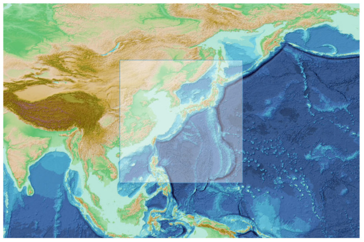 Figure 1
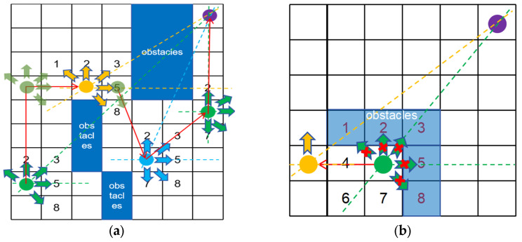 Figure 2
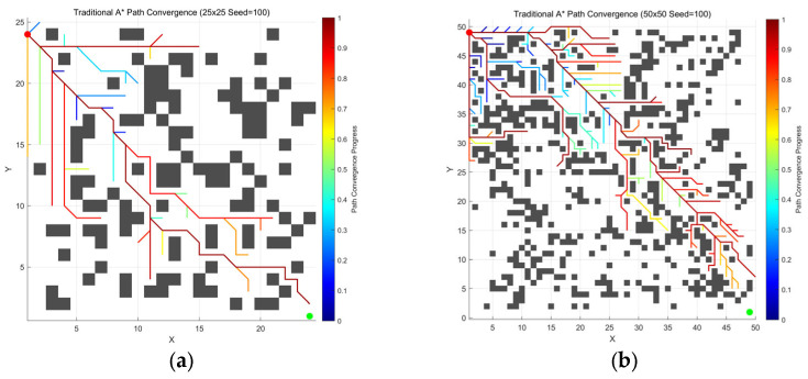 Figure 3
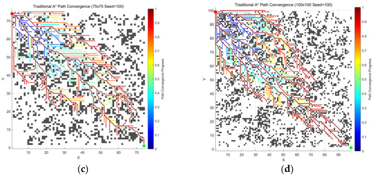 Figure 4
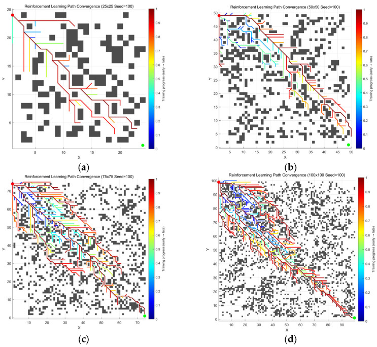 Figure 5
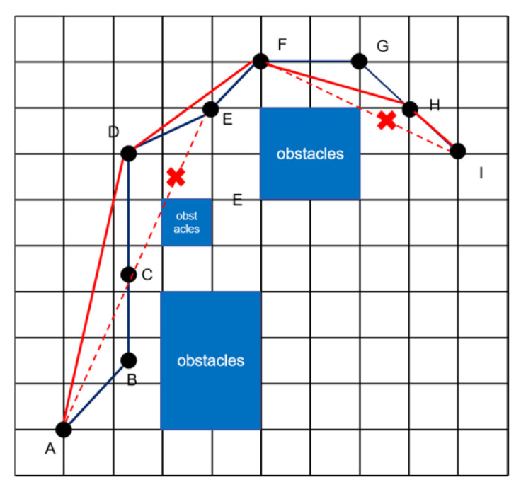 Figure 6
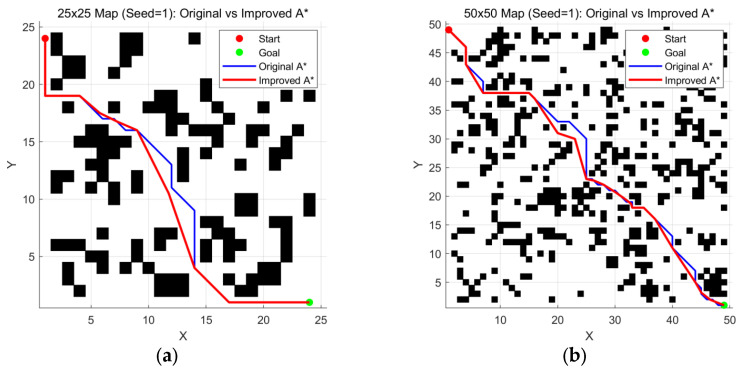 Figure 7
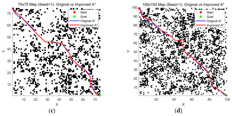 Figure 8
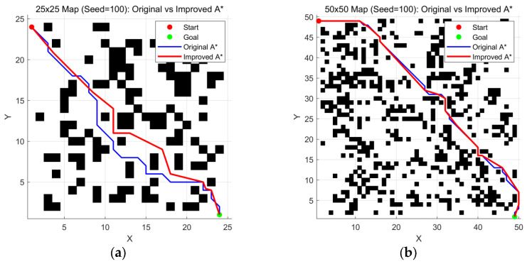 Figure 9
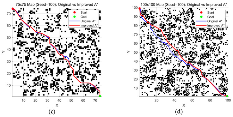 Figure 10
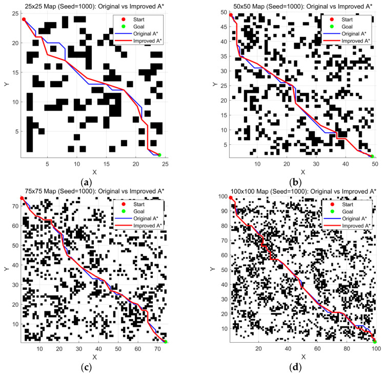 Figure 11
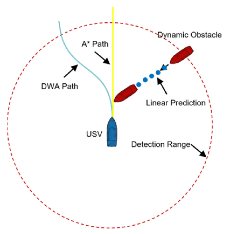 Figure 12
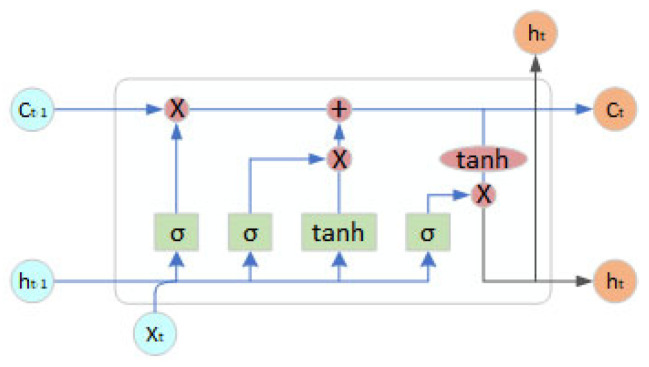 Figure 13
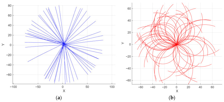 Figure 14
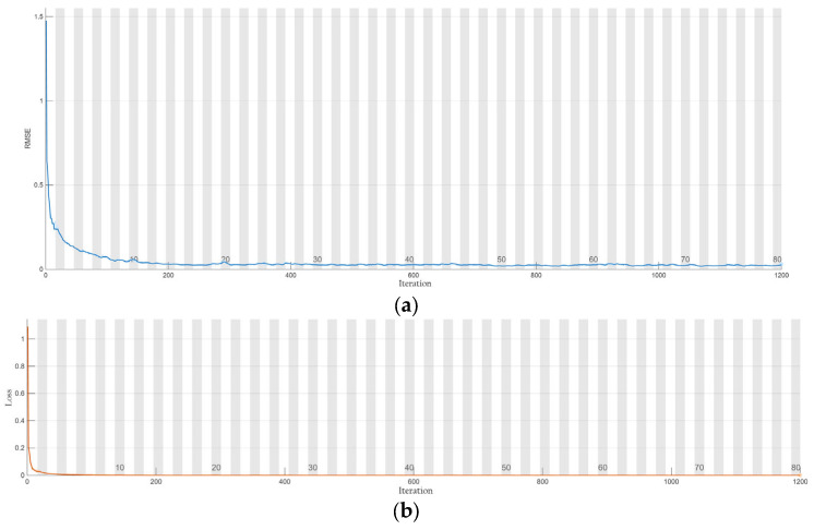 Figure 15
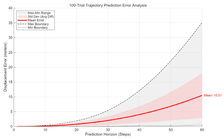 Figure 16
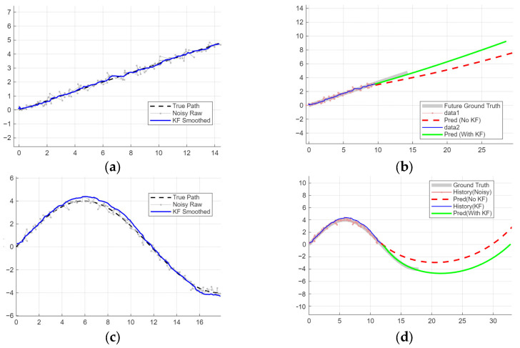 Figure 17
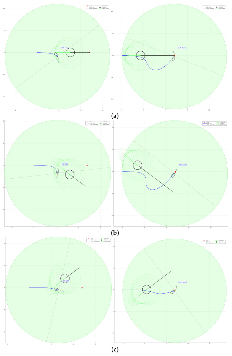 Figure 18
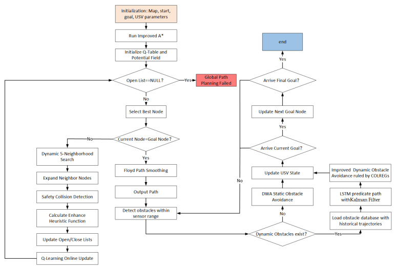 Figure 19
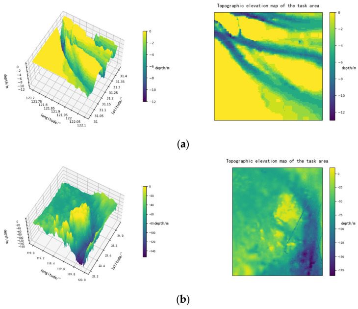 Figure 20
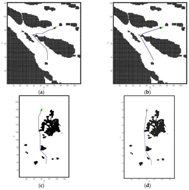 Figure 21
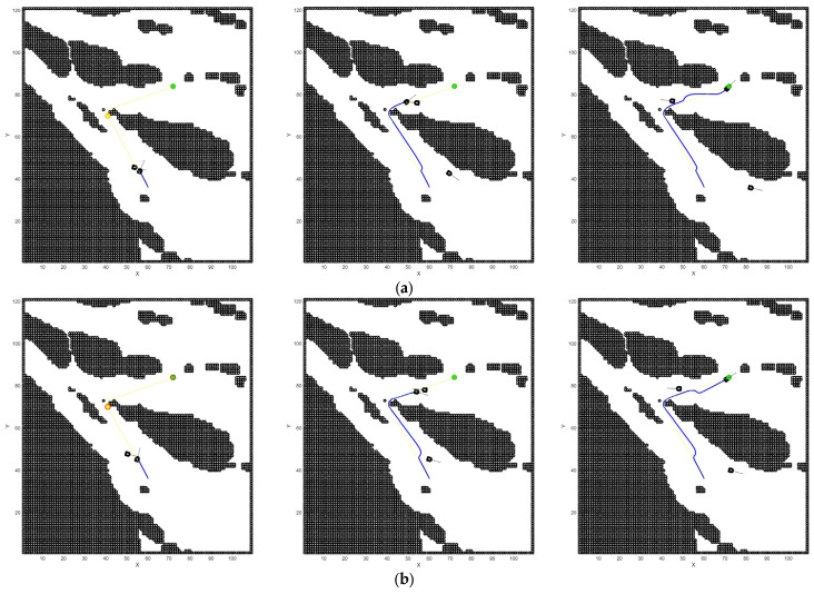 Figure 22
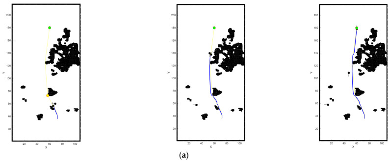 Figure 23
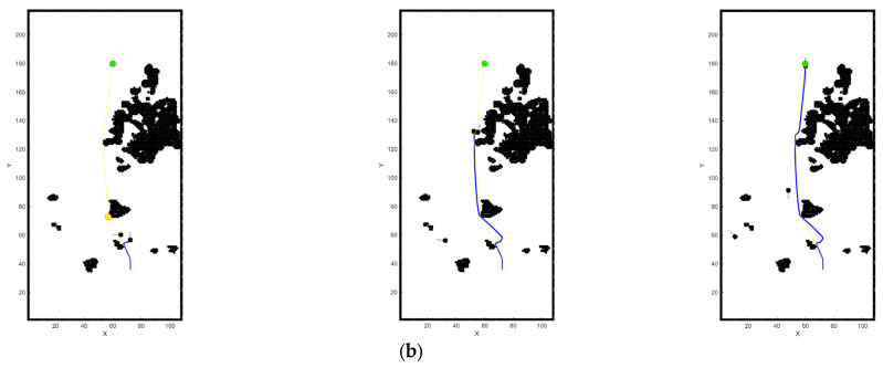 Figure 24
Peer Reviews
No public reviews on file for this paper yet. If you reviewed it on a platform where reviews are public (OpenReview, ICLR, NeurIPS, ICML), you can paste yours below so the community can read it here.
Videos
No videos yet. Explain this paper in a talk, walkthrough, or lecture? Add one.
Taxonomy
TopicsMaritime Navigation and Safety · Robotic Path Planning Algorithms · Ship Hydrodynamics and Maneuverability
1. Introduction
Autonomous systems have become increasingly prevalent in modern maritime applications. As a low-cost and highly maneuverable maritime vehicle, USVs can adapt to most conditions at sea, and trajectory optimization in maritime networks has become a key research focus [1]. Empowered by intelligent algorithms [2], they are capable of performing tasks autonomously under various circumstances. However, safety concerns remain in autonomous path planning for public waters and narrow channels. In the complex and ever-changing marine environment [3], USVs may encounter numerous situations during navigation. Any delays in response or suboptimal path planning can compromise both the safety and efficiency of USVs operations at sea.
The path planning methods for USVs are primarily divided into global path planning and local path planning. Global path planning mainly relies on prior maps, while local path planning depends on obstacle information collected by sensors. Due to the variable and complex maritime conditions [4], it is usually necessary to integrate both global and local path planning to address these challenges.
In global path planning, as summarized by Lixing Liu et al. [5], commonly used algorithms include Dijkstra, A*, RRT, and the particle swarm algorithm, among others. The principles and applicable environments of these algorithms differ. Recent studies have also explored automated path planning strategies for robotic inspection in complex infrastructure environments, providing valuable insights for maritime applications [6]. Comparing these algorithms, A* balances efficiency and optimality. It can find the optimal solution based on a heuristic function and reduces the number of unnecessary nodes to explore by guiding the search direction towards the goal. However, the A* algorithm still has some issues. For instance, in areas close to obstacles, it may produce paths with multiple right-angle turns, resulting in unsmooth trajectories. Many scholars have made improvements and optimizations to the A* algorithm. Yuanmin Liu et al. [7] proposed a time-optimal A* algorithm which enhances the optimal path of the A* algorithm by modifying the heuristic method based on an analytical quantification of time cost. Similarly, Zhi Lin et al. [8] integrated prejudgment planning strategy and redundant inflection point elimination strategy into A-star to improve the quality of the path. The principle of enhancement, drawing inspiration from A*’s heuristic-driven search, has also been applied to a wide range of nature-inspired path planning algorithms. For example, Yujie Huang et al. [9] improved the whale optimization algorithm by incorporating segment learning and adaptive operator selection, which enhanced the algorithm’s search capability. Similarly, Long et al. [10] proposed an improved particle swarm optimization with neighbor adjustment strategies to enhance task scheduling efficiency, which shares similarities with neighborhood search optimization in path planning. In addition, machine learning algorithms have also been employed for path planning. Xiaobing Yu et al. [11] proposed a reinforcement learning-based multi-strategy cuckoo search algorithm. Furthermore, Ren et al. [12] explored multi-agent reinforcement learning with explicit neighborhood backtracking for network-wide control, while Gu and Wang [13] developed a constrained reinforcement learning approach to handle cooperative control in dense obstacle environments, demonstrating the efficacy of RL in complex constraints.
In dynamic environments, conventional collision avoidance algorithms such as Artificial Potential Field (APF) [14], DWA [15,16], and D* are commonly employed. These algorithms offer advantages such as fast computation and high real-time performance. Specifically, the DWA algorithm can effectively incorporate the kinematic constraints of the vehicle to generate rapid responses, making it widely applicable for local obstacle avoidance in various robotic and intelligent systems. However, a key limitation of DWA is that it only evaluates trajectories within a short simulation time window and lacks the capability for complex prediction of dynamic obstacles’ future intentions. To address these shortcomings, numerous researchers have proposed improvements. For instance, Dhong Hun Lee et al. [17] estimated the spatial distribution of obstacles using a Flow Map Field and predicted their future distributions to enhance the obstacle avoidance capability of DWA. Similarly, Hui Chen et al. [18] developed a decision tree-based DWA algorithm that adaptively adjusts its weighting parameters. Furthermore, Chuanbo Wu et al. have integrated machine learning methods with DWA to optimize its reward function, enabling the system to make optimal collision avoidance decisions in complex environments.
In summary, only by integrating global and local path planning [19,20] can a USV achieve a fully autonomous closed-loop navigation route. To address the limitations of the A* and DWA algorithms, we propose a global path optimization and predictive obstacle-avoidance algorithm. The specific improvements are as follows:
- The heuristic function of the A* algorithm is adaptively optimized using a reinforcement learning approach to improve path quality.
- A dynamic five-neighborhood search range is adopted to enhance the algorithm’s search speed.
- An LSTM network, integrated with KF, is employed to predict the trajectories of dynamic obstacles. Enabling the LSTM to provide stable, accurate, and early judgments of obstacle movements to mitigate collision risks.
- The evaluation function of the DWA is reformulated to strictly incorporate International Regulations for Preventing Collisions at Sea. LSTM enables the USVs to execute anticipatory and compliant avoidance maneuvers.
2. Environmental Map
This study employs a grid-based method to model the continuous marine environment. The bathymetric data used for modeling is sourced from GEBCO [21]. By discretizing the continuous environment into regular grids for computational convenience, the algorithm extracts and imports the elevation map model. The overall area (The box-selected area in Figure 1) is defined within the coordinates (100° E and 10° N) to (150° E and 50° N), and the converted output grid file can be generated. The input parameters of the interface can be adjusted to modify the operational area for specific tasks. Experimental studies were conducted in multiple sea areas, yielding distinct results. In the grid, individual points are expanded multi-dimensionally to form impassable obstacle zones, significantly reducing the potential for contact with the vessel hull.
The data utilizes elevation data in the form of a latitude–longitude grid, with a longitude/latitude error of 0.0042 degrees. The USVs model is now initialized and transformed to be compatible with this grid model’s data.
3. Reinforcement A*
3.1. Conventional A*
The conventional A* algorithm [22] utilizes a heuristic function to estimate the cost from the current node to the goal node, thereby guiding the search direction, reducing the search space, and improving search efficiency [23]. By integrating the completeness of Dijkstra’s algorithm [24] with the directional advantages of both Breadth-First Search (BFS) and Greedy Best-First Search (GBFS), the A* algorithm achieves a unique hybrid mechanism. This enables the algorithm not only to find near-optimal paths but also to significantly enhance search efficiency, making it widely applicable in various fields.
The evaluation function for a node in the A* algorithm is defined as shown in Equation (1):
where
- : the actual cost from the start node to the current node ;
- : the heuristic estimated cost from the current node to the goal node.
The key to the A* algorithm lies in the design of the heuristic function. Ideally, should accurately reflect the true cost from the node to the goal. In practical applications, the A* algorithm typically uses the Manhattan distance, Euclidean distance, or Chebyshev distance [25] to approximate .
Equations (2)–(4), respectively, express the Manhattan distance, Euclidean distance, and Chebyshev distance. and represent the coordinate values of the current node and the target node.
3.2. Q-Learning
The Q-learning algorithm is a classic reinforcement learning method belonging to the category of model-free, off-policy control approaches. This algorithm can be applied to any Markov Decision Process (MDP) to approximate an optimal policy [26]. The core of Q-learning lies in its use of temporal difference updates, where iterative estimations are employed to optimize the action-value function. In path planning tasks, a robot selects and executes an action based on the current environmental state, and the environment returns a corresponding reward while transitioning to a new state. If the robot receives a positive reward (+ ), it becomes more likely to choose the same path again in the future; conversely, a negative reward (− ) reduces this tendency [27]. Through continuous feedback, the algorithm progressively refines its strategy over multiple interactions, optimizing decision-making until the policy converges or the task is completed.
where
- : the immediate reward function;
- : the environmental state at the current time step;
- : the action selected under state ;
- : the new state reached after executing action ;
As shown in Equation (5), the probability distribution is determined by the initial state-action estimate at time step t, while the update rule for the optimal value function obtained through iterative computations is defined by the following equation:
where
- : the updated Q-value after taking action , in state , at time t + 1;
- : the discount factor, which balances the importance of immediate rewards and future returns;
- : the maximum Q-value among all possible actions in the next state , and signifies that the action belongs to the set of valid actions in the action space .
When integrating the Q-learning with the A* algorithm, the system continuously selects actions according to policy during each episode to choose optimal actions, achieving learning objectives through iterative optimization of Q-values [28]. Furthermore, as the algorithm undergoes repeated learning, its exploration coefficient gradually decreases with extended training time, thereby maximizing the selection of optimal actions.
3.3. Improved A*
3.3.1. Dynamic Five-Neighborhood Search
The conventional A* algorithm typically employs a four-neighborhood search strategy, considering only four possible movement directions on a two-dimensional plane. To enhance its performance, an improved version introduces an eight-neighborhood (eight-way) search. However, as the eight-way approach often generates redundant nodes, a dynamic five-neighborhood search concept is further incorporated. This refinement effectively reduces redundant nodes during the search process, thereby improving the algorithm’s operational speed and efficiency.
The dynamic five-neighborhood search adaptively adjusts the search direction in real-time, based on the relative positional relationship between the current node and the target point. The specific implementation involves selecting five prioritized expansion directions according to the angle θ between the current node and the target. This strategy not only maintains the completeness of the search but also significantly enhances search efficiency.
When obstacles are detected in all five prioritized neighborhood directions, the algorithm automatically switches to a full eight-neighborhood search to prevent deadlock situations. This adaptive adjustment mechanism ensures the algorithm’s reliability across diverse environments.
As illustrated in Figure 2, the dynamic five-neighborhood search method (Figure 2a) selects five prioritized directions based on the angle θ between the current node and the target. If an unreachable path is encountered (Figure 2b), the algorithm re-selects and explores the previously discarded nodes. The specific node indexing is detailed in Table 1 below:
3.3.2. Reinforcement Learning-Based Adaptive Weighting
The dynamically weighted reinforcement learning algorithm employs an innovative hybrid architecture—the QL-A* algorithm—which integrates the global path planning capability of the conventional A* algorithm with the local optimization ability of Q-learning. By emphasizing real-time dynamic adjustment of the heuristic function, the algorithm continuously learns environmental features during the path planning process and progressively optimizes decision-making strategies. Compared with conventional methods, the improved algorithm demonstrates significant enhancements in path quality, search efficiency, and real-time performance.
The heuristic function is defined as follows:
where
- : the value of the enhanced heuristic function, which integrates the conventional heuristic, potential field guidance, and learned experience;
- : the base heuristic function;
- : the potential field value, generated based on the attraction from the target point to guide the path toward convergence with the goal;
- : the action-value function learned through Q-learning, accumulating historical decision-making experience;
- : the weight coefficient for the potential field, controlling the strength of its guidance;
- : the weight coefficient for the Q-value, adjusting the influence of learned experience.
Design of a Multi-Objective optimization reward function framework:
where
- , , , and : the weight coefficients for each component, namely basic movement cost, progress-toward-goal reward, smoothness penalty, and potential field adjustment, all satisfying the normalization condition .
Table 2 provides a detailed description of each component.
The algorithm employs a lightweight Q-table structure to facilitate experience accumulation across search cycles, with Q-value updates following standard reinforcement learning rules. As shown in Table 2, the reward function is designed to incorporate multiple factors, including movement distance cost, progress reward toward the goal, a slight penalty for diagonal movements, and an adjustment term for potential field variations.
Compared to the conventional A* (Figure 3), the enhanced A* algorithm by leveraging reinforcement learning (Figure 4) exhibits a more efficient search strategy, culminating in a notable decrease in the number of nodes expanded and a higher success rate in directional advancement toward the goal point.
3.3.3. Path Optimization
The initial path generated by the improved A* algorithm still exhibits issues of redundant nodes and excessive turns. To ensure the stability and safety of the navigation system, a path optimization algorithm is employed for path post-processing.
As shown in Figure 5, taking the typical path A → I as an example, the algorithm sequentially evaluates the feasibility of direct connections between adjacent nodes. It checks whether non-consecutive nodes (e.g., A and C, A and D, etc.) can be connected via a straight line without intersecting obstacles. When certain intermediate nodes (e.g., B, C, etc.) are deemed skippable, the system directly connects feasible nodes (e.g., A to D), thereby eliminating redundant nodes.
Additionally, the algorithm incorporates a safety distance threshold. Even if no direct collision with obstacles occurs after removing redundant nodes, a path is still considered invalid if it passes too close to an obstacle (e.g., the direct connection from F to I is too near an obstacle). Through this systematic evaluation and optimization, unnecessary turning points are eliminated, significantly enhancing path continuity and motion efficiency while ensuring the path remains obstacle-free, and navigation reliability is maintained.
3.3.4. Simulation Experiments
The simulation experiments were conducted on the MATLABR2025a platform with a comprehensive testing scheme. Four different map sizes—25 25, 50 50, 75 75, and 100 100—were selected for evaluation. For each map size, three distinct random seeds (Seed = 1, Seed = 100, and Seed = 1000) were used to generate randomized environments, ensuring the statistical significance of the test results.
The experiments compared the performance of the conventional A* algorithm and the improved A* algorithm across multiple test scenarios. In the results, the blue curve represents the path planning trajectory of the conventional A* algorithm, while the red curve corresponds to the planning results of the improved A* algorithm.
As shown in Figure 6 and Table 3, data comparing Conventional A* and Improved A* indicate that on maps with seed = 1, Improved A* achieves significant improvements in path quality.
As shown in Figure 7 and Table 4, the data comparison sustains the superiority of the improved A*, while the quality is maintained at the same level as when the seed = 1.
The experimental results in Figure 6, Figure 7 and Figure 8 and Table 3, Table 4 and Table 5 demonstrate that the improved A* algorithm significantly outperforms the conventional A* algorithm across all performance metrics. Specifically, paths generated by the improved algorithm are on average 5–8% shorter, have 30–45% fewer turning points, and are 50–70% smoother. Additionally, the number of expanded nodes is reduced by around 25–35%. These results conclusively demonstrate the comprehensive advantages of the improved algorithm in terms of path quality, search efficiency, and motion smoothness.
4. Improved DWA
4.1. Kinematic Model
In the DWA algorithm, establishing the motion model is a necessary step for initialization. The establishment of the motion model determines the determination of the sampling space in the DWA algorithm, thereby constraining the range of the motion space. The kinematic model and dynamic window for the next time step are as follows:
The updated position must satisfy the basic requirement of obstacle avoidance. Specifically, the Euclidean distance between the updated position and all obstacles must be greater than or equal to the sum of the USV’s minimum braking distance and the influence radius of the nearest obstacle.
where
- : minimum safe braking distance
- , : obstacle influence radius
- : maximum deceleration
4.2. LSTM
In the DWA algorithm, typically only the vehicle’s own trajectory for the next step is simulated, without predicting the motion trajectories of dynamic obstacles. Consequently, it has weak predictive capability regarding dynamic obstacles and cannot formulate correct steering strategies. As illustrated in Figure 9, if the oncoming vessel is too fast, a collision may occur, posing a high risk. Moreover, COLREGs Rule 15 requires the give-way vessel to avoid crossing ahead of the other vessel.
Accurate prediction is crucial for safe motion planning; for instance, Liang et al. [29] utilized Transformer-based approaches for interaction-aware trajectory prediction in autonomous driving. To capture long-term dependencies in sequence data, advanced architectures like deep residual LSTM networks (ResLNet) have also been proposed [30]. In this study, a sequential prediction model is constructed based on the LSTM network to predict the motion trajectories of dynamic obstacles.
The model takes the incremental changes in historical consecutive positional coordinates as input, with the objective of predicting the positional increments at the next time step, thereby achieving autoregressive prediction of path trends.
The LSTM [31] network is a type of recurrent neural network in which hidden nodes are replaced by LSTM cells (Figure 10). These cells are structured into three gates: the forget gate, the input gate, and the output gate. They are designed to carry relevant information across multiple time steps, avoiding the risks of vanishing or exploding gradients.
The training data in Figure 11 originates from a kinematic simulator designed to replicate obstacle trajectories during autonomous navigation. To emulate real-world conditions, each path ba is subjected to randomized parametric variations, including velocity scaling and heading drift. The detailed training parameters configurations utilized for the LSTM model are presented in Table 6.
The training evolution of the LSTM architecture, illustrated in Figure 12, demonstrates robust convergence characteristics and high numerical precision. The Root Mean Square Error (RMSE) exhibits a rapid decay, stabilizing at approximately 200 epochs. Simultaneously, the loss function plateaus at a negligible magnitude, indicating that the network has successfully minimized the discrepancy between the predicted trajectories and the ground truth without manifesting overfitting.
To assess the model’s generalization capability, we conducted a closed-loop validation utilizing 100 newly generated trajectories, comprising both linear segments and curvilinear maneuvers with steering angles restricted to less than 20°. A comparative analysis between the LSTM-predicted trajectories and the ground truth-summarized in Figure 13 and Table 7 reveals high predictive fidelity within the initial 20-step horizon. However, as the temporal displacement increases, a cumulative divergence becomes evident. Notably, even within the intermediate 10-to-20 step interval, the maximum error metrics exhibit sporadic deviations. To mitigate prediction errors caused by sensor noise and enhance systemic robustness, a Kalman Filter [32] was employed as a dual-stage optimizer: first, to denoise the initial trajectory inputs, and subsequently, to recursively adjust the LSTM-generated outputs against the vehicle’s kinematic constraints.
To evaluate the impact of KF as a front-end trajectory denoising module on the performance of an LSTM-based trajectory prediction model, comparative experiments were conducted under different motion patterns, including straight-line motion and turning maneuvers.
As presented in Figure 14, the predictions based on known path data exhibit reliable regularity and trajectory stability. The KF performs robustly in the data preprocessing stage (Figure 14a,c) and demonstrates a superior ability to smooth and refine the LSTM output trajectories (Figure 14b,d), ensuring more accurate and stable motion trends.
4.3. Adjustment of the Evaluation Function
The evaluation function integrates LSTM-based perception with COLREGs-based decision-making. As shown in Figure 15, the framework uses LSTM to predict the motion of obstacles and create a dynamic risk region. At the same time, it applies COLREGs [33,34] constraints to guide the USV’s heading.
In the conventional DWA, heading is evaluated based solely on the alignment between the robot’s predicted orientation and the target goal. To ensure navigation safety in dynamic environments and strict adherence to COLREGs, an improved heading evaluation function is proposed. The heading evaluation function which integrates a rule−compliance correction term into the standard goal-oriented objective.
The improved heading evaluation function is defined as follows:
where
- : the basic goal-alignment score;
- : the dynamic weight for distance-dependent;
- : the weight for heading.
By incorporating the predicted dynamic obstacle information and the USV’s current state, this module identifies the encounter situation. Then, dynamically adjusts the heading score, imposing penalties on non-compliant maneuvers to ensure the selected trajectory adheres to maritime traffic rules.
The predicted trajectory generated by the LSTM is mapped into a dynamic danger zone, illustrated as the green dashed area in Figure 15. The evaluation function is adjusted to penalize any candidate trajectory intersecting this zone, ensuring the USVs proactively avoid the obstacle’s future path.
where
- : a collection of parameters, where denotes the -th parameter and denotes the scores in EvalDB for heading, obstacle distance, and velocity, respectively; denotes the penalty score for proximity to the dynamic obstacle zone predicted by LSTM. This penalty appears when near dynamic obstacles, increases linearly within the zone, and is set to 0 outside the zone;
- : weight for each parameter;
- : number of motion candidates.
5. A*-DWA Fusion
5.1. Algorithmic Flowchart
We integrated both global and local path planning algorithms to propose a combined A*-DWA. The specific flowchart is illustrated in Figure 16. The algorithm enhances its global path search capability through dynamic five-neighborhood exploration and adaptive weight adjustment via reinforcement learning, while also achieving a shorter and smoother route through path optimization.
The local algorithm predicts the short-term motion trajectories of dynamic obstacles through LSTM, and by incorporating the improved DWA algorithm, it enhances predictive avoidance of obstacles, thereby improving navigation safety.
5.2. Simulation
We conducted algorithmic simulation tests using the two maps shown in Figure 17, performing experiments in both narrow waterways and open sea areas. During initialization, a default expansion range was set to prevent failures in local path planning.
Figure 18 and Table 8 indicate that the Aalgorithm, when enhanced with a dynamic environment layer and reinforcement learning, can reduce the number of expanded nodes and optimize the path strategy. Furthermore, the secondary optimization algorithm further enhances path smoothness and reduces the number of turns. Through the improved Aalgorithm, the SUV consumes less energy during missions, leading to higher efficiency.
In narrow waters, the conventional algorithm demonstrates significant limitations. It cannot anticipate the trajectory of dynamic obstacles, selecting only the optimal route for the current moment without considering the obstacle’s movement in the next instance. In Figure 19a, the conventional DWA algorithm comes to a complete stop because the updated DWA position falls within the hazard zone of a dynamic obstacle, with no feasible direction to proceed, thereby resulting in a trapped and dangerous situation. In contrast, the improved DWA, as shown in Figure 19b, is capable of predicting the trajectory of dynamic obstacles in advance and ensures that its heading does not intersect with that of the obstacles, leading to significantly better performance.
In open waters shown in Figure 20, the conventional DWA algorithm, much like in narrow waters, cannot ensure the USVs remain in a relatively safe state in the next moment. Moreover, in head-on encounter situations, it fails to initiate turns proactively, which poses certain safety risks.
Through simulation comparisons, it is observed that the conventional DWA often struggles with slow planning and inaccuracies when encountering fast-moving dynamic obstacles, and may even cause the USVs to stop within hazardous areas. In contrast, the improved DWA algorithm, by incorporating LSTM-based path prediction and modifications to the evaluation function, enables the USVs to perform local obstacle avoidance proactively and safely. As a result, the improved DWA demonstrates superior obstacle-avoidance performance in the presence of dynamic obstacles, both in narrow waterways and open sea areas.
6. Discussion
By integrating reinforcement learning with the traditional A* algorithm, the selection of the heuristic function in A* can be enhanced. This approach reduces action consumption through a dynamic five-neighborhood search and optimizes the final path to generate the shortest and most cost-effective route. When combined with an LSTM-based path prediction algorithm, it mitigates risks posed by dynamic obstacles and improves local planning stability. This path planning algorithm is adaptable to most environments, thereby significantly enhancing the safety of USVs in complex maritime areas.
However, if compared with other hybrid planners, such as RL combined with Model Predictive Control (MPC), reveals notable distinctions in weaknesses. MPC-based solutions operate by solving optimization problems at every time step. This continuous calculation allows them to strictly handle kinematic constraints and ensure dynamic feasibility, even under environmental disturbances. Our algorithm exhibits reduced robustness against extreme dynamic disturbances when compared to RL-based methods.
Second, the current simulation environment assumes an idealized kinematic model and does not explicitly account for environmental disturbances such as strong winds, waves, and ocean currents. In real-world maritime operations, these disturbances introduce significant drift and uncertainty that can affect the USV’s global path planning and tracking precision. Although the Kalman Filter currently employed addresses sensor noise, it does not fully compensate for the complex non-linear dynamics introduced by severe sea states.
Future Work Future research will focus on incorporating a high-fidelity hydrodynamic model to simulate wind and wave effects. Additionally, we aim to explore more robust cost functions that scale with prediction uncertainty to further enhance safety in complex, stochastic environments.
The reference list from the paper itself. Each links out to its DOI / PubMed record.
- 1Yao Y. Xiao W. Miao P. Chen G. Yang H. Chae C.B. Wong K.K. UAV-Relay-Aided Secure Maritime Networks Coexisting with Satellite Networks: Robust Beamforming and Trajectory Optimization IEEE Trans. Wirel. Commun.2026252342235810.1109/TWC.2025.3596136 · doi ↗
- 2Gu C. Deng D. Xiang C. Risk-aware model predictive control framework for collision avoidance in unmanned surface vehicles Ocean Eng.202534212295410.1016/j.oceaneng.2025.122954 · doi ↗
- 3Sun X. Wang G. Fan Y. Mu D. Collision avoidance control for unmanned surface vehicle with COLRE Gs compliance Ocean Eng.202326711326310.1016/j.oceaneng.2022.113263 · doi ↗
- 4Chen Z. Zhang Y. Zhang Y. Nie Y. Tang J. Zhu S. A Hybrid Path Planning Algorithm for Unmanned Surface Vehicles in Complex Environment with Dynamic Obstacles IEEE Access 2019712643912644910.1109/ACCESS.2019.2936689 · doi ↗
- 5Liu L. Wang X. Yang X. Liu H. Li J. Wang P. Path planning techniques for mobile robots: Review and prospect Expert Syst. Appl.202322712025410.1016/j.eswa.2023.120254 · doi ↗
- 6Yang Z. Shu J. Jiang J. Han W. Wang Y. Zhao L. Bai Y. Automated path-planning strategy for robotic inspection of underground utilities based on building information model Comput. Aided Civ. Infrastruct. Eng.2025405554557510.1111/mice.70107 · doi ↗
- 7Liu Y. Gao X. Wang B. Fan J. Li Q. Dai W. A passage time–cost optimal A* algorithm for cross-country path planning Int. J. Appl. Earth Obs. Geoinf.202413010390710.1016/j.jag.2024.103907 · doi ↗
- 8Lin Z. Wu K. Shen R. Yu X. Huang S. An Efficient and Accurate A-Star Algorithm for Autonomous Vehicle Path Planning IEEE Trans. Veh. Technol.2024739003900810.1109/TVT.2023.3348140 · doi ↗