Genomic Prediction and Genome‐Wide Association Analysis of Heat Tolerance for Milk Yield in Buffaloes Using a Reaction Norm Model
Gabriela Stefani, Mário Luiz Santana, Lenira El Faro, Humberto Tonhati

TL;DR
This study uses genomic data to improve predictions of milk yield in buffaloes under heat stress and identifies genes linked to heat tolerance.
Contribution
The study introduces genomic prediction models for heat tolerance in buffaloes and identifies candidate genes for milk yield under thermal stress.
Findings
Genomic models increased heritability estimates and breeding value accuracy under heat stress.
Genes ESRRG, IGSF5, and PCP4 were identified as strong candidates for heat tolerance in milk yield.
Genomic data improved modeling of genotype-by-environment interactions for milk yield.
Abstract
The aim of this study was to evaluate the impact of incorporating genomic information on the estimation of genetic (co)variance components and the accuracy of breeding values for milk yield under varying thermal environments, and to identify SNPs associated with genes that play significant roles in heat tolerance. We analysed 58,070 test‐day milk yield records from 3459 first lactations, collected between 1987 and 2018 from six herds. Genotypic data consisted of 870 animals genotyped for 45,405 SNP markers. Climatic data were obtained from INMET and combined into a temperature‐humidity index (THI). Breeding values for test‐day milk yield across THI values and days in milk were estimated using both genomic and pedigree‐based random regression animal models. The model incorporating genomic information yielded higher estimates of heritability and additive genetic variance, along with…
Genes, proteins, chemicals, diseases, species, mutations and cell lines named across the full text — each resolved to its canonical identifier and authoritative record.
Click any figure to enlarge with its caption.
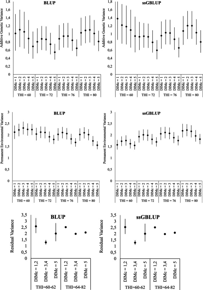 FIGURE 1
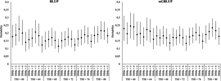 FIGURE 2
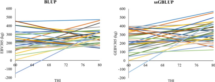 FIGURE 3
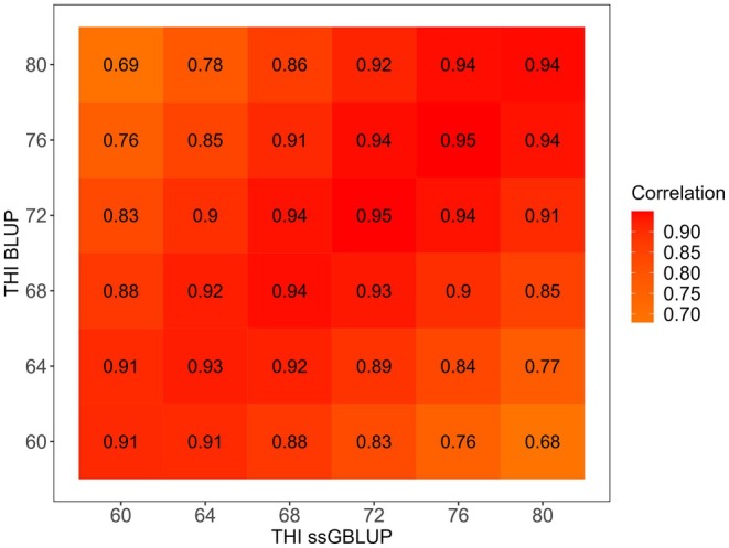 FIGURE 4
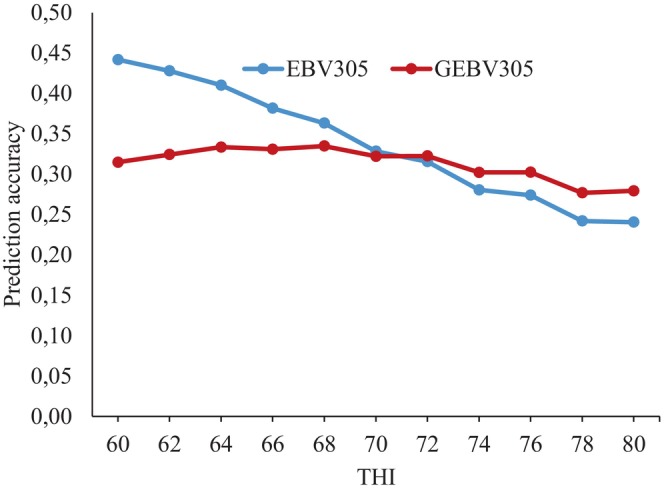 FIGURE 5
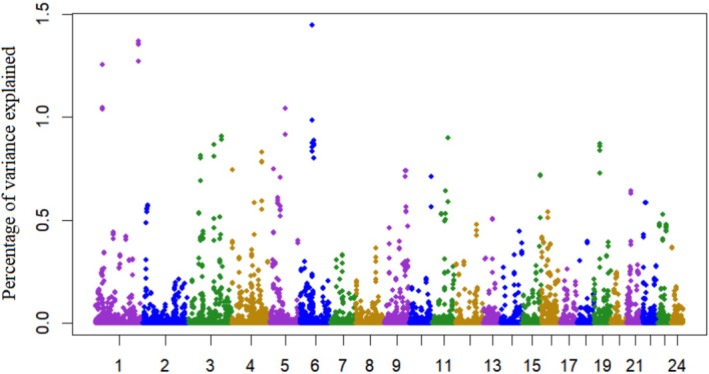 FIGURE 6
| ssGBLUP | BLUP | |
|---|---|---|
|
| ||
| L | 1.65 (0.24) | 1.35 (0.24) |
| S | 0.17 (0.04) | 0.15 (0.04) |
| L–S covariance | −0.19 (0.06) | 0.02 (0.06) |
| L–S genetic correlation | −0.35 (0.10) | 0.05 (0.14) |
| S/L ratio | 0.11 (0.03) | 0.11 (0.04) |
|
| ||
| L | 2.98 (0.17) | 3.32 (0.20) |
| S | 0.01 (0.00) | 0.02 (0.00) |
| L–S covariance | 0.11 (0.01) | −0.12 (0.01) |
| L–S genetic correlation | 0.68 (0.03) | ‐0.51 (0.03) |
| S/L ratio | 0.00 (0.00) | 0.00 (0.00) |
| ID | Símbolo | Nome | Crom. | Pos. inicial | Pos. final |
|---|---|---|---|---|---|
| 102393698 | ESRRG | Oestrogen‐related receptor gamma | 5 | 60724148 | 61418016 |
| 112585283 | LOC112585283 | Not labelled | 5 | 60829111 | 60866752 |
| 112585410 | TRNAC‐ACA | Transfer RNA cysteine (anticodon ACA) | 5 | 61015447 | 61015518 |
| 102392178 | LOC102392178 | Glutamic acid‐rich SH3 domain‐binding protein | 1 | 184095392 | 184171535 |
| 112586660 | LOC112586660 | Not labelled | 1 | 184226779 | 184256279 |
| 102395407 | LOC102395407 | Not labelled | 1 | 184232895 | 184240093 |
| 102395629 | B3GALT5 | Beta‐1,3‐galactosyltransferase 5 | 1 | 184279283 | 184318251 |
| 102396557 | IGSF5 | Immunoglobulin superfamily member 5 | 1 | 184393961 | 184448054 |
| 102397063 | PCP4 | Purkinje cell protein 4 | 1 | 184505825 | 184572722 |
| 102411501 | FRG1 | FSHD region gene 1 | 1 | 26395523 | 26409563 |
| 112587455 | LOC112587455 | U2‐30 small nucleolar RNA | 1 | 26401246 | 26401318 |
| 112587456 | LOC112587456 | U2‐19 small nucleolar RNA | 1 | 26401452 | 26401531 |
| 112587490 | LOC112587490 | SNORA81 small nucleolar RNA | 1 | 26630162 | 26630317 |
| 102415368 | BCAR3 | BCAR3 adaptor protein, NSP family member | 6 | 49547993 | 49700908 |
| 112585621 | LOC112585621 | Not labelled | 6 | 49693740 | 49701029 |
| 102415695 | FNBP1L | Formalin‐binding protein 1 | 6 | 49714736 | 49839300 |
| 112585912 | LOC112585912 | U6 RNA spliceosomal | 6 | 49753312 | 49753418 |
| 112585623 | LOC112585623 | 60S ribosomal protein pseudogene L23a | 6 | 49766701 | 49767207 |
| 112585622 | LOC112585622 | 60S ribosomal protein pseudogene L9 | 6 | 49803601 | 49804312 |
| 112585854 | LOC112585854 | SNORA16B small nucleolar RNA/SNORA16A family | 6 | 49865716 | 49865848 |
| 102416237 | DR1 | Transcriptional repressive regulator 1 | 6 | 49878865 | 49900876 |
| 102401316 | LOC102401316 | Myosin light regulatory polypeptide 9 pseudogene | 6 | 49951657 | 49952552 |
| 102416561 | CCDC18 | Coiled‐coil domain 18 | 6 | 49978486 | 50090546 |
- —Fundação de Amparo à Pesquisa do Estado de São Paulo10.13039/501100001807
- —Conselho Nacional de Desenvolvimento Científico e Tecnológico10.13039/501100003593
Peer Reviews
No public reviews on file for this paper yet. If you reviewed it on a platform where reviews are public (OpenReview, ICLR, NeurIPS, ICML), you can paste yours below so the community can read it here.
Videos
No videos yet. Explain this paper in a talk, walkthrough, or lecture? Add one.
Taxonomy
TopicsEffects of Environmental Stressors on Livestock · Genetic and phenotypic traits in livestock · Reproductive Physiology in Livestock
Introduction
1
Buffaloes ( Bubalus bubalis ) are recognised for their hardiness and adaptability to hot and humid climates. According to Damasceno et al. (2010), buffaloes represent an attractive option in areas where cattle struggle to adapt, contributing to their increasing use in various regions worldwide. The buffalo population in Brazil totals approximately 1 million head (IBGE 2017), with the majority being raised on pasture under adverse climatic conditions. Although buffaloes are known for their remarkable hardiness, several studies have shown that heat stress significantly impacts the productive performance of dairy buffaloes (Choudhary and Sirohi 2019; Nasr 2017; Pawar et al. 2013; Stefani et al. 2021).
Environmental differences may contribute to variations in daughter records, leading to re‐ranking of bulls across different environments (Hammami et al. 2009; Hayes et al. 2016). This phenomenon is known as genotype by environment (G × E) interaction, where different genotypes respond differently to varying environments (Falconer and Mackay 1996). The impact of challenging environmental factors, particularly climate change and its associated heat stress responses, can result in re‐rankings of sires under different climatic conditions. Therefore, in order to remain competitive across diverse climates worldwide, international dairy cattle breeding programs should incorporate G × E interaction effects into their genetic evaluations (Ravagnolo and Misztal 2000).
Over the past decade, several studies have analysed genotype by environment interactions (G × E) for milk yield traits using random regression models (RRM) (Hammami et al. 2013; Carabaño et al. 2014). RRM allows for modelling the effect of a genotype as a function of time (e.g., days in milk) and environment (e.g., temperature‐humidity index; THI), enabling the detection of G × E interactions through differences in genetic (co)variance components for various combinations of DIM and THI (Bohmanova et al. 2008; Brügemann et al. 2011). According to Santana et al. (2015), G × E interactions can lead to significant selection errors between different environments, thereby hindering genetic progress for the trait. In this context, Stefani et al. (2021) studied Brazilian dairy buffaloes and found significant G × E interactions when applying a pedigree‐based random regression model to milk yield while incorporating a function for THI. Additionally, genetic variance for heat tolerance enables selection for genetically heat‐tolerant animals, which can help maintain high productivity while ensuring survival under adverse conditions (Dash et al. 2016), making it an important objective for genetic improvement programs.
Traditional selection methods, which use pedigree‐based relationship matrices, can achieve long‐term genetic gain. However, traditional pedigree‐based selection methods are characterised by a slower rate of genetic progress due to reduced accuracy, since they cannot capture Mendelian sampling variation when animals lack phenotypic records and predictions rely solely on parental information, as well as due to longer generation intervals (Goddard et al. 2011; Brito 2021). Furthermore, given that progeny testing is one of the most costly and time‐consuming phases of a breeding program, there is a need to develop more efficient strategies to model G × E interactions and improve prediction accuracy (Morais Júnior et al. 2018). The single‐step approach allows for the simultaneous integration of phenotypic records, genealogy and available genomic data (Aguilar et al. 2010; Christensen and Lund 2010; Legarra et al. 2009). By combining this approach with random regression models, it is possible to accelerate genetic progress, reduce generation intervals, and estimate more accurate breeding values compared to pedigree‐based analyses alone (Kang et al. 2017; Legarra and Ducrocq 2012; Zhang et al. 2016). However, to date, no studies have incorporated the single‐step approach into an RRM to model the effects of heat stress on milk production in buffaloes.
Another application of genomic random regression models (RRM) is the genetic characterisation of complex phenotypes and the identification of candidate genes in proximity to or in linkage disequilibrium with markers across environments through genome‐wide association studies (GWAS; Mota et al. 2020). The weighted single‐step GWAS is a method that allows for the estimation of SNP effects using GEBVs predicted by the single‐step approach (Wang et al. 2012). This method enables the efficient implementation of complex models, such as RRM, for genomic prediction of longitudinal traits (Kang et al. 2017) and accommodates unequal variances for SNPs, leading to improved precision in estimating SNP effects (Wang et al. 2012). Therefore, genetic progress could be accelerated by identifying the single nucleotide polymorphisms (SNPs) responsible for heat tolerance in milk yield and utilising them in marker‐assisted selection. However, there are currently no reports of candidate gene mapping studies conducted within a genomic reaction norms framework in buffaloes.
The main objectives of this study were: (1) to compare genetic (co)variance components and the prediction accuracies of breeding values for milk yield in the first lactation under different thermal environment conditions, using random regression models with and without genomic information, applying ssGBLUP and BLUP, respectively; (2) to investigate the effect of including genomic information on the genetic components related to heat tolerance in the first lactation; and (3) to identify SNP markers associated with genes that have significant effects on heat tolerance in milk yield.
Materials and Methods
2
Phenotypes
2.1
The phenotypic, genotypic and genealogical data used in this study were provided by the Department of Animal Science, Faculdade de Ciências Agrárias e Veterinárias—UNESP, Jaboticabal, SP, Brazil. After editing, a total of 53,113 test‐day milk yield records from 3179 first lactations of Murrah buffaloes, collected between 1987 and 2018, were used in the analyses. These records came from six herds located in three Brazilian states: Rio Grande do Norte (43.5%), São Paulo (42.8%) and Ceará (13.7%). The animals were predominantly raised on pasture in regions characterised by humid tropical and semi‐arid climates. The herds have been under selection for approximately 20 years, primarily focused on males, based on the national breeding value for 305‐day milk yield.
Test‐day milk yield records were obtained between Days 5 and 305 of the first lactation, with each lactation meeting at least the following five criteria: a minimum duration of 90 days; the first test‐day occurring before 75 days of lactation; at least four test‐days; the animal aged between 22 and 60 months; and the animal having at least one known parent. Contemporary groups (CG) were defined as herd‐year‐month of the test‐day and had to contain at least four animals. This definition has been widely adopted in genetic evaluations of dairy buffaloes and cattle in Brazil (Aspilcueta‐Borquis et al. 2012; Santana et al. 2015, 2017), ensuring comparability with the national evaluation system. Records with values exceeding 3.0 standard deviations above or below the CG mean were excluded. Based on the results of a preliminary analysis, six classes of days in milk (DIM) with 50‐day intervals were defined: 5–54, 55–104, 105–154, 155–204, 205–254 and 255–305 days. The pedigree file was constructed by tracing 7 generations back from the individuals with phenotypic or genotypic information, totaling 4522 animals.
Genotypes
2.2
After genotype quality control, a total of 45,405 single nucleotide polymorphism (SNP) data points from 870 Murrah dairy buffaloes were used in the analyses, of which 782 had phenotypic records. The genotyped animals were distributed among the three states as follows: 35.4% in São Paulo, 62.9% in Rio Grande do Norte and 1.7% in Ceará. The herds were partially connected through sires used in more than one herd and through genomic relationships among animals from different states. The animals were genotyped using the Affymetrix Axiom Buffalo genotyping chip (90 k SNP; Thermo Fisher Scientific, Wilmington, DE). The marker positions for this chip are based on the University of Adelaide water buffalo assembly map (UOA WB v. 1, Affymetrix, 2016). SNP quality control was performed using the preGSf90 program (Aguilar et al. 2010), applying the following exclusion criteria for markers: unmapped; duplicated; not autosomal; call rates below 0.90; minor allele frequency (MAF) less than 0.05; and deviation from Hardy–Weinberg equilibrium greater than 0.15. Additionally, only samples with call rates greater than 0.90 were included in the analyses.
Environmental Descriptor
2.3
Meteorological data were provided by the Instituto Nacional de Meteorologia (INMET, Brasília‐DF, Brazil). Climatic variables were measured at three standardised times (09:00, 15:00 and 21:00 h) daily at four weather stations located within 70 km of the farms. The station closest to each herd was designated as the reference station for that herd. Data collection procedures at the weather stations are standardised nationwide, following the recommendations of the World Meteorological Organization. The variables dry‐bulb temperature (T; in °C) and relative air humidity (RH; in %) for the same day as the test day were combined into a temperature‐humidity index (THI) using the equation described by NRC (1971):
This formula was adopted because it is suited to the climatic variables available at Brazilian weather stations (T and RH). Additionally, several studies have demonstrated the effectiveness of this formula for similar studies (Bohmanova et al. 2008; Brügemann et al. 2011, 2012). The average daily THI, calculated as the mean of the six days (five days before and the test‐day itself), was assigned to each test‐day milk yield record. The selection of six days was based on the results of a preliminary analysis, which showed that the 6‐day average explained a greater portion of the variability in milk production. A similar approach was adopted by Bohmanova et al. (2008), Santana et al. (2017) and Stefani et al. (2021). The THI values were then rounded to the nearest multiple of 2, with the first class starting at THI = 60 and the last class starting at THI = 80, resulting in a total of 11 classes.
Statistical Analyses
2.4
The genetic parameters for test‐day milk yield across DIM and THI values were estimated using a random regression model (RRM). Fixed and random regressions on DIM were modelled using Legendre polynomials of order 3 (intercept, linear, quadratic, cubic), based on the approach used by Aspilcueta‐Borquis et al. (2012). The linear fixed and random regressions on THI were modelled using Legendre polynomials of order 1, which is equivalent to a classical reaction norm model (intercept and linear terms). Based on the results of a preliminary analysis, the residual variance was assumed to be heterogeneous across lactation (DIM: classes 1, 2–4 and 5–6) and THI values (THI: classes 60–62, 64–80), resulting in six different combinations. The random regression animal model was described as follows:
where yjklmn is the mth TD milk yield record of the lth animal; FIXEDk is the kth combination of fixed effects of GC (defined as above), classes of combination between milking frequency and DIM, regression coefficient for the linear and quadratic effects of cow's age at calving in months, regression coefficients for the linear, quadratic and cubic effects of DIM nested within classes of herd‐2 years of calving and regression coefficient for the linear effect of THI nested within DIM; βln the nth random regression coefficient for the additive genetic effect of animal l by DIM; γln the nth random regression coefficient for the permanent environmental effect of animal l by DIM; δln the nth random regression coefficient for the additive genetic effect of animal l by THI; εln the nth random regression coefficient for the permanent environmental effect of animal l by THI; q the number of regression coefficients; ωnd the nth orthogonal Legendre polynomial corresponding to DIM d; ωnt the nth orthogonal Legendre polynomial corresponding to THI t; and eijklm the random residual effect. The (co)variance structure follows:
where A is the numerator relationship matrix; Gβ and Gδ are (co)variance matrices of the random regression coefficients for additive genetic effects by DIM and THI, respectively; Gβδ and Gδβ the covariance matrices for additive genetic effects for combinations of DIM and THI; ⊗ the Kronecker product; Pγ and Pε the (co)variance matrices of the random regression coefficients for permanent environmental effects by DIM and THI, respectively; Pγε and Pεγ the covariance matrices for permanent environmental effects for combinations of DIM and THI; and σeo2 the residual variance, with o ranging from 1 to 6 according to the number of residual class; Il is an identity matrix of appropriate size for the permanent environmental effect (l is the number of animals with records) and Im an identity matrix of appropriate size for the residual (m is the number of TD records). In single‐step genomic best linear unbiased prediction models as developed by Aguilar et al. (2010), H is the hybrid matrix that combines the pedigree‐based numerator relationship matrix A with the genomic relationship matrix G, as developed by Aguilar et al. (2010). The inverse of H was defined as:
where: A is the numerator relationship matrix; A22 is the pedigree relationship matrix among genotyped animals; G is the genomic relationship matrix, constructed by an iterative algorithm, that was completely described by Wang et al. (2012). These iterations increase the weights of SNPs with large effects and decrease those with small effects, essentially regressing them to the mean (Wang et al. 2014).
In the BLUP analysis, the pedigree‐based relationship matrix A was used instead of the H matrix. The analyses were conducted using the GIBBS3F90 program from the BLUPF90 software package (Misztal et al. 2002) using a Bayesian framework via Gibbs sampling. The prior distributions for all random effects were inverse Wishart distributions. The analysis consisted of a single chain of 1,000,000 cycles, with a conservative burn‐in period of 600,000 cycles and a thinning interval of 100 cycles. Thus, 4000 samples were effectively used. Convergence was determined by Geweke's diagnostic (Geweke 1991), visual inspection of the posterior chains of the parameters, and assessing the autocorrelation and effective sample size of the posterior parameter samples.
Estimation of Genetic Parameters
2.5
The additive genetic and permanent environmental (co)variances matrices were calculated as ФGФ′ and ФPФ′, respectively, where Ф was a matrix of Legendre polynomial functions for DIM or THI classes. The elements on the diagonals were additive genetic (σa2) and permanent environmental (σpe2) variances for each DIM or THI class. The covariances between DIM i and THI j were calculated as ФiGβδФ′j and ФiPγεФ′j. Consequently, the test‐day milk yield heritability for the i th DIM class within the j th THI class was:
where σaβδij and σpγεij are covariances of ith DIMc and jth level of THI for additive genetic and permanent environmental effects, respectively; σaβⅈ2 and σaδj2 are the additive genetic variances of ith DIMc and jth level of THI, respectively; σpγi2 and σpεj2 are permanent environmental variances of ith DIMc and jth level of THI, respectively; and σe2 is the residual variance.
Genomic Predictions Based on RRM
2.6
The additive genetic effect of the random regression coefficients was used to derive the genomic estimated breeding value (GEBV), for each DIM and THI. Therefore, the EBV and GEBV of an animal i were calculated as:
where: α^i′ is the vector of the orthogonal regression coefficients of animal i for additive genetic effects (coefficients corresponding to DIM and THI); ϕjk is a vector of orthogonal coefficients evaluated in the THI j and DIM k. Thus, the GEBVs for 305‐day milk yield (GEBV305) were calculated as the sum of the GEBVs from Days 5 to 305 of lactation at a THI value of interest. Accordingly, the conventional EBV based on the pedigree relationship matrix for 305‐day milk yield was EBV305.
To study the differences in thermal sensitivity and the effects of including genomic information on selection, we analysed the response pattern of EBV305 and GEBV305 across the THI scale for 30 top‐ranking bulls, selected from the total of 85 bulls with at least 10 daughters. These 30 bulls were chosen based on the highest EBV305 values under thermoneutral conditions (THI = 72) to allow a clearer graphical visualisation of re‐ranking. In addition, Pearson's correlation was calculated between the EBV305 and the GEBV305 of all bulls with at least 10 daughters (a total of 85 bulls) across the THI scale.
Validation of Genomic and Pedigree‐Based Predictions
2.7
To compare prediction accuracies between BLUP and ssGBLUP across the THI scale, a validation scheme was implemented using young animals. To simulate genomic selection at a very young age, when the animal's own performance data is not yet available, a reduced dataset was created by excluding the phenotypes of the younger animals (test‐days recorded from 2010). The validation population comprised the 150 youngest genotyped animals. This reduced dataset was then used to estimate EBV305 using the BLUP approach and GEBV305 using the ssGBLUP approach for the animals in the validation population, using the variance components previously estimated from the complete dataset.
To assess the prediction bias in each thermal environment, the linear regression coefficients of the GEBV305 and EBV305 for the validation animals, obtained from the reduced dataset, were compared with their EBV305 obtained from the complete dataset, for each THI. The linear regression model is given by:
where: yc refers to the EBV305 of the validation population obtained by the complete dataset in a THI of interest; b0 and b1 refer to the intercept and linear regression coefficients; âr refers to the GEBV305 or EBV305 of the validation animals, obtained by the reduced dataset in a THI of interest; and e refers to the residue. The b1 was used as an indicator of bias. The validation accuracy (r) was calculated from the coefficient of determination (r ^2^) of the regression equation.
GWAS for Heat Tolerance
2.8
The PostGSf90 software (Aguilar et al. 2014) was used to estimate SNP effects for the slope coefficient of the reaction norm, which reflects the animal's ability to respond to heat stress. Two iterations were performed to estimate the genetic variance explained by five adjacent SNP windows, aiming to identify potential genome regions with larger effects on heat stress tolerance. A threshold of 1.0% of the total genetic variance explained by each genomic window was applied to define the important genomic regions associated with the trait.
The reference genome UOA WB v. 1 was used to search for candidate genes potentially associated with the selected SNPs. The Genome Data Viewer tool of the buffalo genome, available on the National Center for Biotechnology Information (NCBI) website (http://www.ncbi.nlm.nih.gov), was used to identify the genes. Genes mapped within 200 kb upstream or downstream of the important SNPs were considered, as this range captures the regulatory and functional regions near the SNPs, though not necessarily contained within them (Peñagaricano et al. 2013).
Results and Discussion
3
Figure 1 presents the variance components of test‐day milk yield across DIM and THI classes, estimated by BLUP and ssGBLUP. In both analyses, considerable variation was observed along the THI scale, providing clear evidence of genotype‐by‐environment (G × E) interaction. By displaying results for all DIM × THI combinations rather than only weighted averages by THI, it became evident that these interactions are not uniform but stage‐dependent, reflecting the combined influence of thermal environment and lactation dynamics. Similar conclusions have been reported in dairy cattle, where heat stress responses are strongly modulated by lactation stage (Brügemann et al. 2011; Santana et al. 2017).
Posterior means (•) and 95% highest posterior density regions (vertical bars) of additive genetic variance (kg2), permanent environmental variance (kg2) and residual variance (kg2) of test‐day (TD) records for different combinations of days in milk classes (DIMc) and temperature‐humidity index (THI), estimated under BLUP (left) and ssGBLUP (right) methods.
Additive genetic variance (Figure 1) followed a U‐shaped profile across the THI gradient, with lower values around thermoneutral conditions (THI ≈ 72) and higher values at both mild (THI = 60) and heat‐stress levels (THI ≥ 76). Stage‐specific patterns were also evident: at low THI, variance tended to decrease from early to mid‐lactation, whereas at high THI, variance increased toward mid‐to‐late lactation. These results suggest that genetic differences become more evident under environmental extremes, particularly when physiological demands peak, consistent with previous findings in cattle and buffaloes (Bohmanova et al. 2008; Stefani et al. 2021; Marai and Haeeb 2010). Importantly, ssGBLUP systematically increased additive genetic variance and accentuated these gradients, in agreement with studies showing that genomic information strengthens genetic links across environments and improves G × E detection (Nguyen et al. 2016; Garner et al. 2016; Hayes et al. 2016). It should also be noted that Legendre polynomials are known to inflate variance estimates at the extremes of the trajectory. Therefore, part of the higher variances observed at the beginning and end of lactation may reflect this statistical property rather than biological processes. Still, the hypothesis of stronger selection pressure in early lactation remains plausible. Future studies using non‐parametric regressors (e.g., splines) could help clarify this issue.
Permanent environmental variance (Figure 1) was higher under BLUP than under ssGBLUP, indicating that when genomic information was not included, part of the variability was absorbed by this component. By redistributing variance toward the additive genetic part, ssGBLUP reduced the relative weight of persistent non‐genetic effects, consistent with reports in dairy cattle that genomic models improve the partitioning of variance components (Misztal et al. 2009; Brügemann et al. 2011). Interestingly, BLUP suggested a gradual decrease in permanent variance with increasing THI, whereas ssGBLUP revealed a more heterogeneous profile across DIM × THI combinations, suggesting that persistent non‐genetic effects may also be modulated by environmental challenges.
Residual variances (Figure 1) showed comparable magnitudes between models, but BLUP exhibited larger oscillations across DIM classes, particularly in early lactation, and a pronounced peak under mild THI (60–62). In contrast, ssGBLUP produced more stable estimates across environments, suggesting that genomic information captured part of the heterogeneity that would otherwise inflate the residual component. Notably, residual variances did not systematically increase with THI, indicating that the models successfully allocated the effects of heat stress into additive genetic and permanent environmental components rather than into unexplained variability. Similar observations have been reported in studies where explicit modelling of THI reduced residual noise by accounting for environmental heterogeneity (Bohmanova et al. 2008; Bernabucci et al. 2014; Stefani et al. 2021).
Figure 2 shows the heritability estimates of test‐day milk yield across DIM and THI classes. Heritability ranged from 0.12 to 0.30, indicating low to moderate genetic control of the trait. A U‐shaped profile was again observed across THI, with the lowest values around thermoneutral conditions (THI ≈ 72) and higher estimates under both mild and heat‐stress conditions. This suggests that extreme environments amplify the expression of genetic differences, whereas thermoneutral conditions—where most selection historically occurred—tend to reduce variability (Nguyen et al. 2016). Across lactation, heritability was generally higher in early stages, decreased during mid‐lactation, particularly under thermoneutral THI, and increased again toward late lactation under heat stress. These stage‐specific fluctuations highlight the combined effect of thermal load and physiological demand, as also noted in Holstein cattle (Brügemann et al. 2011; Santana et al. 2017; Carabaño et al. 2014). Finally, ssGBLUP provided slightly higher and more stable heritability estimates compared with BLUP, reinforcing the advantage of genomic information for reducing noise and improving the accuracy of genetic parameter estimation (Garner et al. 2016; Hayes et al. 2016).
Posterior means (•) and 95% highest posterior density regions (vertical bars) of heritability estimates of test‐day (TD) records for different combinations of days in milk classes (DIMc) and temperature‐humidity index (THI) estimated under BLUP (left) and ssGBLUP (right) methods.
For both ssGBLUP and BLUP methods, the slope coefficient of the reaction norm, which represents the animal's ability to respond to heat stress, exhibited greater additive genetic variance than permanent environmental variance (Table 1). This suggests that heat stress tolerance has a stronger genetic than environmental component, making it a feasible target for selection. Incorporating genomic information into the reaction norm model increased the additive genetic variance of both the intercept and slope by approximately 22% and 13%, respectively. It also resulted in lower standard deviations, indicating more precise estimates—likely due to enhanced relationship coefficient estimation. The slope/intercept ratios were similar between the two methods, indicating a meaningful G × E interaction. The genetic correlation between the intercept and slope was near zero in the BLUP method, suggesting no association between the general milk yield level and heat stress response. In contrast, ssGBLUP produced a moderate and negative correlation, indicating that animals with higher production levels tend to exhibit lower heat tolerance. This increased correlation under ssGBLUP suggests more pronounced re‐ranking of animals across different environments. These patterns were further reflected in the distribution of breeding values across THI environments, as illustrated in Figure 3.
Response pattern along the temperature–humidity index (THI) scale of the 305‐day milk yield estimated breeding values (EBV305) and genomic estimated breeding values (GEBV305) for the top 30 bulls (with at least 10 daughters), ranked by EBV305 at THI = 72. [Colour figure can be viewed at wileyonlinelibrary.com]
Figure 3 illustrates the response patterns of EBV305 and GEBV305 for the 30 top‐ranking bulls, evaluated across the THI scale. The varying sensitivities of animals to environmental changes influenced the distribution of breeding values in both BLUP and ssGBLUP analyses. Clear re‐rankings were observed across thermal environments, emphasising the presence of G × E interaction and highlighting the risk of selection errors if heat sensitivity is not properly modelled. The ssGBLUP approach showed more pronounced re‐ranking, which is consistent with the greater additive genetic variance observed for the slope of the reaction norm (Table 1). This reinforces the role of genomic information in capturing individual differences in heat tolerance and improving the accuracy of selection under variable climatic conditions.
Figure 4 presents the Pearson correlations between EBV305 and GEBV305 for the 85 most‐used sires across THI values. These correlations revealed considerable variation in genetic evaluations when genomic information was included, particularly under extreme THI conditions. Since fewer test‐day records are typically available at the extremes of the thermal scale, pedigree‐based BLUP relies more heavily on ancestral information, which limits accuracy. In contrast, ssGBLUP incorporates genomic relationships that strengthen genetic links among animals across herds and environments, thereby providing more robust predictions. This explains why the largest discrepancies between EBV and GEBV occurred at high THI values, where genomic information plays a crucial role in maintaining connectedness and reducing bias. Such findings are consistent with previous reports in dairy cattle, where genomic models improved the accuracy of breeding values in less‐represented or stressful environments (Hayes et al. 2016; Garner et al. 2016). These discrepancies highlight the environments where genomic data provide the greatest advantage, a trend that is consistent with the validation results presented in Figure 5.
Pearson correlations between EBV305 and GEBV305 for 305‐day milk yield of 85 bulls with at least 10 daughters. [Colour figure can be viewed at wileyonlinelibrary.com]
Prediction accuracies of EBV305 and GEBV305 for 305‐day milk yield across THI values. Accuracies were calculated as the correlation between breeding values predicted in the validation scheme (using the reduced dataset of the youngest genotyped animals) and those obtained from the complete dataset. [Colour figure can be viewed at wileyonlinelibrary.com]
Figure 5 presents the prediction accuracies obtained from the validation procedure described in the 2. Materials and Methods section, using the reduced dataset and the validation population of the 150 youngest genotyped animals. Here, accuracies refer to the correlation between breeding values predicted in the validation scheme (using the reduced dataset) and those obtained from the complete dataset. These accuracies, estimated for each THI class, allow the comparison between the BLUP and ssGBLUP approaches under different thermal environments. Overall, the prediction accuracies of EBV305 from BLUP decreased as THI increased (Figure 5). At lower THI values, accuracies appeared higher, likely because phenotypic information was scarce and the predictions from pedigree alone did not diverge substantially from those obtained using the full dataset. As THI increased, the larger amount of phenotypic information available highlighted the limitations of pedigree‐only predictions, leading to reduced accuracies. In contrast, GEBV305 accuracies remained stable across the THI scale, likely because the H matrix in ssGBLUP allows genomic similarity to strengthen connections between animals not related by pedigree. While BLUP generally produced higher accuracies, ssGBLUP accuracies remained more stable across THI values due to the additional genomic information strengthening connectedness, and yielded more accurate GEBVs at higher THIs (> 70). Given that 72.5% of the test‐day records in this study were collected at THIs > 70, ssGBLUP appears to be a suitable method for predicting GEBVs in these buffalo herds. These results are consistent with studies in Holsteins showing that genomic prediction models perform particularly well under challenging or less‐represented environments (Hayes et al. 2016; Morais Júnior et al. 2018).
Figure 6 shows the results of the genome‐wide association study (GWAS) for the slope coefficient of the reaction norm, which reflects the animal's sensitivity to heat stress in milk yield. Consistent with the variance component results presented in Table 1, the GWAS highlighted that heat tolerance has a detectable genetic basis. However, most genomic windows explained less than 1% of the total additive genetic variance, underscoring the highly polygenic nature of the trait. This pattern is in agreement with previous studies in cattle, which also reported dispersed genomic signals for heat stress tolerance rather than strong major loci (Garner et al. 2016; Nguyen et al. 2016). Nevertheless, some genomic regions exceeded the 1% threshold and were selected for further investigation. The candidate genes identified within these regions are listed in Table 2 and provide valuable insights into the biological mechanisms underlying heat stress responses, complementing the quantitative genetic evidence and offering opportunities for future genomic selection strategies.
Proportion of additive genetic variance of the slope coefficient explained by 5‐SNP windows for test‐day milk yield. The x‐axis represents chromosomes (in colour), the y‐axis represents marker contributions, and the grey horizontal line marks the 1.0% threshold for candidate genomic regions. [Colour figure can be viewed at wileyonlinelibrary.com]
The genes located in the most important regions are listed in Table 2. Several of these genes are related to hormonal responses and the regulation of internal and external stimuli. ESRRG, a steroid hormone receptor, plays a crucial role in thermogenesis (Ahmadian et al. 2018). Gu et al. (2020) associated ESRRG with responses to stressful environments in native Chinese chickens. ESRRG has also been linked to milk yield in buffalo (De Camargo et al. 2015) and cattle (Venturini et al. 2014). MYL9 (LOC102401316) has been associated with panting in heat‐stressed Jersey cows (Wang et al. 2021) and immune responses to heat stress in chickens (Monson et al. 2018). SH3BGRL3 (LOC102392178) has been linked to heat‐tolerant cows (Garner 2017). IGSF5 is associated with reproductive functions and showed altered expression in heat‐stressed pregnant sows (Seibert 2018; Zhao et al. 2021). PCP4, which modulates calmodulin–calcium binding, is involved in heat stress signalling in plants (Wu and Jinn 2012) and has been linked to inflammation during heat stress in dairy cows (Shahzad et al. 2015). Despite these findings, further research is needed to elucidate the biological and functional pathways of these genes, which could provide valuable markers for genomic selection programs aiming to improve heat tolerance in buffaloes.
Conclusion
4
The ssGBLUP method resulted in higher estimates of heritability and additive genetic variance, along with greater accuracies under heat stress conditions. It also provided a better model for genotype‐by‐environment (G × E) interaction affecting milk production in buffaloes, making it a suitable alternative for predicting breeding values. This study is the first to include genomic information in the assessment of heat stress tolerance in buffaloes, filling a gap in the literature. Models that incorporate G × E interaction should be integrated into current selection schemes to identify animals with better heat tolerance. Several genes were identified within the candidate genomic regions, and further studies are required to explore the biological and functional pathways of these genes influencing heat stress tolerance in milk production.
Conflicts of Interest
The authors declare no conflicts of interest.
The reference list from the paper itself. Each links out to its DOI / PubMed record.
- 1Aguilar, I. , I. Misztal , and S. Tsuruta . 2010. “Short Communication: Genetic Trends of Milk Yield Under Heat Stress for US Holsteins.” Journal of Dairy Science 93, no. 4: 1754–1758. 10.3168/jds.2009-2756.20338455 · doi ↗ · pubmed ↗
- 2Aguilar, I. , I. Misztal , S. Tsuruta , A. Legarra , and H. Wang . 2014. “PREGSF 90–POSTGSF 90: Computational Tools for the Implementation of Single‐Step Genomic Selection and Genome‐Wide Association With Ungenotyped Individuals in BLUPF 90 Programs.” World Congress on Genetics Applied to Livestock Production (WCGALP).
- 3Ahmadian, M. , S. Liu , S. M. Reilly , et al. 2018. “ERRγ Preserves Brown Fat Innate Thermogenic Activity.” Cell Reports 22, no. 11: 2849–2859.29539415 10.1016/j.celrep.2018.02.061PMC 5884669 · doi ↗ · pubmed ↗
- 4Aspilcueta‐Borquis, R. R. , F. R. Araujo Neto , F. Baldi , D. J. Santos , L. G. de Albuquerque , and H. Tonhati . 2012. “Genetic Parameters for Test‐Day Yield of Milk, Fat and Protein in Buffaloes Estimated by Random Regression Models.” Journal of Dairy Research 79: 272–279.22444071 10.1017/S 0022029912000143 · doi ↗ · pubmed ↗
- 5Bernabucci, U. , S. Biffani , L. Buggiotti , A. Vitali , N. Lacetera , and A. Nardone . 2014. “The Effects of Heat Stress in Italian Holstein Dairy Cattle.” Journal of Dairy Science 97, no. 1: 471–486.24210494 10.3168/jds.2013-6611 · doi ↗ · pubmed ↗
- 6Bohmanova, J. , I. Misztal , S. Tsuruta , H. D. Norman , and T. J. Lawlor . 2008. “Genotype by Environment Interaction due to Heat Stress.” Journal of Dairy Science 91, no. 2: 840–846.18218772 10.3168/jds.2006-142 · doi ↗ · pubmed ↗
- 7Brito, L. F. 2021. “Genetic and Genomic Evaluation of Livestock for Resilience to Climate Variability.” Frontiers in Genetics 12: 667.
- 8Brügemann, K. , E. Gernand , U. König von Borstel , and S. König . 2012. “Defining and Evaluating Heat Stress Thresholds in Different Dairy Cow Production Systems.” Archives Animal Breeding 55: 13–24.