The role of optical coherence tomography in the evaluation of para-chiasmal lesions: a systematic review and meta-analysis
Khai Shin Alva Lim, Wen Xu Abel Tng, Wei De Bryan Theng, Bernett Teck Kwong Lee, Chee Fang Chin, Kelvin Zhenghao Li, Heather E. Moss

TL;DR
This study reviews how optical coherence tomography can help assess vision impacts from brain tumors near the optic chiasm and predict post-surgery visual outcomes.
Contribution
A systematic review and meta-analysis of OCT's role in diagnosing and predicting outcomes for para-chiasmal lesions.
Findings
Patients with para-chiasmal lesions had significantly thinner retinal nerve fiber layers compared to controls.
The inferior quadrant of the peripapillary RNFL showed the greatest thinning in affected patients.
Pre-operative pRNFL thickness was higher in patients with good visual recovery after surgery.
Abstract
While magnetic resonance imaging is currently the primary diagnostic tool for pituitary tumors, optical coherence tomography (OCT) may be used in evaluating the visual pathway impact of these lesions. This study evaluates the utility of OCT in patients with chiasmal compression from para-chiasmal lesions and determines its role in predicting visual field outcomes post-operatively. A search of five databases identified OCT studies in patients with neoplasms affecting the optic chiasm. Meta-analyses compared i) healthy controls versus patients, ii) good versus poor visual recovery post-operatively, and iii) patients with visual field defects (VFDs) versus those without. Standardized mean differences (SMDs) and mean differences (MDs) were used. A review of 97 studies (5,300 patient eyes and 2,209 controls) demonstrated significantly thinner peripapillary retinal nerve fiber layer…
Genes, proteins, chemicals, diseases, species, mutations and cell lines named across the full text — each resolved to its canonical identifier and authoritative record.
Click any figure to enlarge with its caption.
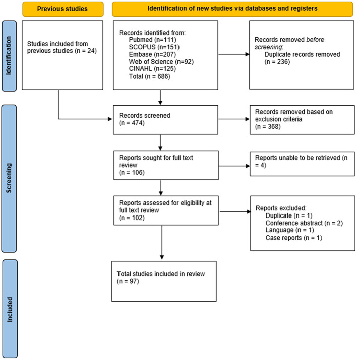 Figure 1
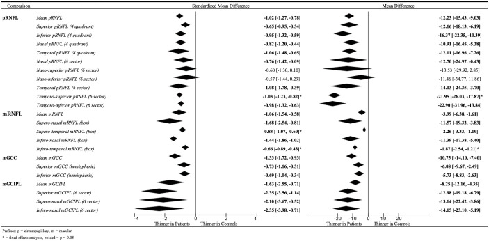 Figure 2
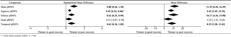 Figure 3
| Study authors | Comparison | Comparisons | Diagnosis | Control eyes | Patient eyes |
|---|---|---|---|---|---|
| Agarwal 2021 ( | Case–control | Healthy vs. patient | PA | 24 | 24 |
| Akashi 2014 ( | Case–control | Healthy vs. patient | Mixed | 49 | 89 |
| Akdogan 2022 ( | Case–control | Healthy vs. patient, prolactin levels | PA | 30 | 32 |
| Altun 2017 ( | Case–control | Healthy vs. patient, micro vs. macroadenoma | PA | 72 | 68 |
| Batur 2023 ( | Case–control | Healthy vs. patient | PA | 38 | 36 |
| Bozzi 2024 ( | Prospective | Over time | PA | 40 | |
| Cennamo 2015 ( | Case–control | Healthy vs. patient | PA | 43 | 33 |
| Cennamo 2020 ( | Case–control | Healthy vs. patient, pre- and post-op | PA | 28 | 14 |
| Cennamo 2021 ( | Prospective | Over time, post-op | PA | 16 | |
| Chen 2023 ( | Case–control | Healthy vs. patient | PA | 45 | 24 |
| Chou 2022 ( | Case–control | Healthy vs. patient | PA | 27 | 27 |
| Chung 2020 ( | Prospective | Pre- and post-op, normal and thin RNFL | PA | 262 | |
| Dallorto 2020 ( | Case–control | Healthy vs. patient, optic neuropathy vs. no optic neuropathy | PA | 17 | 16 |
| Danesh Meyer 2015 ( | Prospective | Over time, normal and thin RNFL | PA | 213 | |
| de Araujo 2017 ( | Case–control | Healthy vs. patient | PA | 30 | 37 |
| Donaldson 2022 ( | Retrospective | Healthy vs. patient, differing VFD, VFD vs. no VFD | Mixed | 53 | |
| Duru 2016 ( | Case–control | Healthy vs. patient, micro vs. macroadenoma | PA | 58 | 76 |
| Ergen 2023 ( | Case–control | Healthy vs. patient, chiasmal distortion | Mixed | 210 | 92 |
| Garcia 2014 ( | Retrospective | Pre- and post-op | Mixed | 38 | |
| Ghezala 2021 ( | Case–control and prospective | Healthy vs. patient, pre- and post-op, chiasmal compression | Mixed | 24 | 32 |
| Glebauskiene 2018 ( | Case–control | Healthy vs. patient, suprasellar extension | PA | 154 | 154 |
| Hernandez-Echvarria 2022 ( | Case–control and prospective | Healthy vs. patient, pre- and post-op | PA | 57 | 35 |
| Iegorova 2019 ( | Case–control and retrospective | Healthy vs. patient, chiasmal compression | Mixed | 76 | 20 |
| Iqbal 2020 ( | Prospective | Pre- and post-op | PA | 40 | |
| Jeon C 2019 ( | Retrospective | Pre- and post-op, normal and thin RNFL | Mixed | 216 | |
| Jeon H 2021 ( | Case–control | Healthy vs. patient, VFD vs. no VFD | Mixed | 47 | 57 |
| Jeon H 2022 ( | Retrospective | Pre- and post-op, good and poor outcomes | Mixed | 25 | |
| Jorstad 2021 ( | Prospective | Development of VFD, over time | Mixed | 19 | |
| Ju 2019 ( | Retrospective | Optic tract edema vs. no edema | Mixed | 212 | |
| Kawaguchi 2019 ( | Retrospective | Pre- and post-op, good and poor outcomes | Mixed | 120 | |
| Lei 2023 ( | Case–control | Healthy vs. patient, compressive ON vs. glaucomatous ON | Mixed | 72 | 36 |
| Kurian 2022 ( | Prospective | Pre- and post-op | PA | 58 | |
| Lang 2021 ( | Case–control | Good and poor outcomes, controls used for rsfMRI | PA | 42 | 19 |
| Lee E 2015 ( | Case–control | Healthy vs. patient, compressive ON vs. glaucomatous ON | Mixed | 131 | 73 |
| Lee G 2020 (1) ( | Case–control | Healthy vs. patient, good and poor outcomes | Mixed | 100 | 100 |
| Lee G 2020 (2) ( | Case–control | Healthy vs. patient, good and poor outcomes | Mixed | 57 | 42 |
| Lee G 2020 (3) ( | Case–control | Healthy vs. patient | Mixed | 36 | 35 |
| Lee G 2021 (1) ( | Case–control | Healthy vs. patient, pre- and post-op | Mixed | 62 | 44 |
| Lee J 2016 ( | Retrospective | Pre- and post-op | CP | 111 | |
| Levchenko 2020 ( | Case–control | Healthy vs. patient | PA | 20 | 30 |
| Li XC 2022 ( | Case–control | PA vs. glaucoma | Mixed | 74 | |
| Loo 2013 ( | Retrospective | Normal and thin RNFL | Mixed | 14 | |
| Mambour 2021 ( | Retrospective | Pre- and post-op | Mixed | 23 | |
| Mangan 2021 ( | Case–control | Healthy vs. patient, normal and thin RNFL, pre- and post-op | Mixed | 29 | 14 |
| Mavilio 2022 ( | Case–control | Healthy vs. patient | PA | 12 | 14 |
| Mello 2022 ( | Case–control | Healthy vs. patient | Mixed | 33 | 40 |
| Meyer 2022 ( | Prospective | Good and poor outcomes | Mixed | 216 | |
| Mimouni 2019 ( | Case–control | Compressive ON vs. glaucomatous ON | Mixed | 31 | |
| Monteiro 2010 ( | Case–control | Healthy vs. patient | Mixed | 35 | 35 |
| Monteiro 2013 ( | Case–control | Healthy vs. patient | PA | 25 | 25 |
| Monteiro 2014 ( | Case–control | Healthy vs. patient | Mixed | 33 | 36 |
| Moon C-H (1) 2011 ( | Prospective | Healthy vs. patient, pre- and post-op | Mixed | 19 | 20 |
| Moon C-H (2) 2011 ( | Prospective | Healthy vs. patient, pre- and post-op | Mixed | 18 | 20 |
| Moon J 2020 ( | Case–control | Healthy vs. patient | PA | 47 | 22 |
| Moura 2010 ( | Case–control | Healthy vs. patient | Mixed | 40 | 40 |
| Nair 2024 ( | Prospective | Pre- and post-op, good and poor outcomes | PA | 66 | |
| Nakamura 2012 ( | Case–control | Healthy vs. patient | Mixed | 26 | 64 |
| Ogmen 2021 ( | Case–control | Healthy vs. patient | PA | 63 | 36 |
| Ohkubo 2012 ( | Case–control | Healthy vs. patient (post-op) | Mixed | 23 | 33 |
| Orman 2021 ( | Case–control | Healthy vs. patient (pre-VFD) | PA | 41 | 35 |
| Ozcan 2022 ( | Case–control | Healthy vs. patient, pre- and post-op | PA | 17 | 17 |
| Pang 2022 ( | Case–control | Healthy vs. patient | PA | 29 | 29 |
| Pang 2023 ( | Case–control | Healthy vs. patient, chiasmal compression | PA | 106 | 106 |
| Pang 2024 ( | Retrospective | Pre- and post-op | PA | 56 | |
| Park 2021 ( | Retrospective | Good and poor outcomes | PA | 144 | |
| Pekel 2014 ( | Case–control | Healthy vs. patient | PA | 60 | 60 |
| Phal 2016 ( | Prospective | Pre- and post-op, good and poor outcomes | Mixed | 17 | |
| Poczos 2019 ( | Prospective | Pre- and post-op | Mixed | 32 | |
| Poczos 2022 ( | Prospective | Pre- and post-op | Mixed | 32 | |
| Qiao 2016 (1) ( | Prospective | Pre- and post-op, transsphenoidal vs. transcranial | PA | 42 | |
| Qiao 2016 (2) ( | Prospective | Pre- and post-op | PA | 46 | |
| Rudman 2024 ( | Retrospective | Pre- and post-op | PA | 78 | |
| Sahin 2017 ( | Case–control | Healthy vs. patient | PA | 33 | 40 |
| Santorini 2021 ( | Case–control | VFD vs. no VFD | Mixed | 88 | |
| Sasagawa 2023 ( | Case–control | Chiasmal compression | Mixed | 138 | |
| Saxena 2015 ( | Prospective | Pre- and post-op | PA | 39 | |
| Shinohara 2022 ( | Retrospective | Pre- and post-op, optic nerve bending | Mixed | 50 | |
| Singha 2024 ( | Retrospective | Pre- and post-op, VFD vs. no VFD | Mixed | 70 | |
| Sousa 2017 ( | Case–control | Healthy vs. patients | PA | 27 | 43 |
| Suh 2021 ( | Retrospective | VFD vs. no VFD | Mixed | 41 | |
| Sun 2017 ( | Case–control | Healthy vs. patients | PA | 38 | 39 |
| Sun 2020 ( | Case–control | Healthy vs. patients | PA | 38 | 43 |
| Suzuki 2020 ( | Case–control | Healthy vs. patients | Mixed | 33 | 42 |
| Tang 2022 (1) ( | Case–control | Good and poor outcomes | PA | 25 | 25 |
| Tang 2022 (2) ( | Case–control | Healthy vs. patients, chiasmal compression | PA | 100 | 41 |
| Thammakumpee 2022 ( | Retrospective | Pre- and post-op, VFD vs. no VFD, good vs. poor outcome | PA | 36 | |
| Tieger 2017 ( | Case–control | Healthy vs. patients | Mixed | 45 | 45 |
| Ueda 2015 ( | Case–control | Healthy vs. patients | Mixed | 53 | 72 |
| Wang G 2021 ( | Case–control | Healthy vs. patients, VFD vs. no VFD | Mixed | 31 | 34 |
| Wang M 2020 ( | Prospective | Pre- and post-op | Mixed | 462 | |
| Wang M 2021 ( | Prospective | Pre- and post-op, normal and thin RNFL | Mixed | 456 | |
| Wang X 2022 ( | Case–control | Healthy vs. patients | PA | 40 | 40 |
| Xia 2022 ( | Case–control | Pre- and post-op, good and poor outcomes | PA | 81 | |
| Yang 2016 ( | Case–control | Healthy vs. patients | Mixed | 64 | 64 |
| Yoneoka 2015 ( | Prospective | Pre- and post-op, good and poor outcomes | Mixed | 70 | |
| Yoo 2020 ( | Retrospective | Good and poor outcomes | Mixed | 79 | |
| Yum 2016 ( | Retrospective | Healthy vs. patient vs. NTG | PA | 77 | 32 |
| Total | 5,300 | 2,209 |
| Study authors | Scan model | Technology utilized |
|---|---|---|
| Agarwal 2021 ( | Zeiss Cirrus HD 4000 | Spectral domain |
| Akashi 2014 ( | Topcon OCT 2000 | Spectral domain |
| Akdogan 2022 ( | Optovue RTVue XR Avanti | Spectral domain |
| Altun 2017 ( | Heidelberg Spectralis OCT | Spectral domain |
| Batur 2023 ( | Heidelberg Spectralis OCT | Spectral domain |
| Bozzi 2024 ( | Unclear | Unclear |
| Cennamo 2015 ( | Optovue RTVue-100 | Spectral domain |
| Cennamo 2020 ( | Optovue | Spectral domain |
| Cennamo 2021 ( | Optovue RTVue | Spectral domain |
| Chen 2023 ( | Optovue RTVue XR Avanti | Spectral domain |
| Chou 2022 ( | Optovue RTVue XR Avanti | Spectral domain |
| Chung 2020 ( | Zeiss Cirrus HD | Spectral domain |
| Dallorto 2020 ( | Zeiss Cirrus HD and Optovue RTVue XR Avanti | Spectral domain |
| Danesh Meyer 2015 ( | Zeiss Stratus | Time domain |
| de Araujo 2017 ( | Heidelberg Spectralis OCT | Spectral domain |
| Donaldson 2022 ( | Zeiss Cirrus 600 | Spectral domain |
| Duru 2016 ( | Optovue RTVue-100 | Spectral domain |
| Ergen 2023 ( | Optovue RTVue XR Avanti | Spectral domain |
| Garcia 2014 ( | Zeiss Stratus | Time domain |
| Ghezala 2021 ( | Zeiss Cirrus HD 5000 | Spectral domain |
| Glebauskiene 2018 ( | Nidek RS-3000 Advance | Spectral domain |
| Hernandez-Echvarria 2022 ( | Zeiss Cirrus 5000 | Spectral domain |
| Iegorova 2019 ( | Optopol Revo NX | Spectral domain |
| Iqbal 2020 ( | Optovue | Spectral domain |
| Jeon C 2019 ( | Heidelberg Spectralis OCT | Spectral domain |
| Jeon H 2021 ( | Zeiss Cirrus HD | Spectral domain |
| Jeon H 2022 ( | Zeiss Cirrus | Spectral domain |
| Jorstad 2021 ( | Nidek RS-3000 | Spectral domain |
| Ju 2019 ( | Heidelberg Spectralis OCT | Spectral domain |
| Kawaguchi 2019 ( | Nidek RS-3000 and Zeiss Stratus 3000 | Spectral domain and time domain |
| Lei 2023 ( | Optovue RTVue XR | Spectral domain |
| Kurian 2022 ( | Topcon DRI OCT Triton plus | Swept source |
| Lang 2021 ( | Zeiss Cirrus HD 4000 | Spectral domain |
| Lee E 2015 ( | Heidelberg Spectralis OCT | Spectral domain |
| Lee G 2020 (1) ( | Heidelberg Spectralis OCT | Spectral domain |
| Lee G 2020 (2) ( | Zeiss Cirrus HD | Spectral domain |
| Lee G 2020 (3) ( | Zeiss Cirrus HD | Spectral domain |
| Lee G 2021 (1) ( | Zeiss Cirrus HD OCT and Topcon DRI OCT Triton Plus | Spectral domain and swept source |
| Lee J 2016 ( | Zeiss Cirrus HD | Spectral domain |
| Levchenko 2020 ( | Zeiss Cirrus HD 5000 | Spectral domain |
| Li XC 2022 ( | Topcon DRI OCT Triton | Swept source |
| Loo 2013 ( | Zeiss Stratus | Time domain |
| Mambour 2021 ( | Zeiss Cirrus HD 5000 | Spectral domain |
| Mangan 2021 ( | OTI Spectral OCT | Spectral domain |
| Mavilio 2022 ( | Zeiss Cirrus 500 | Spectral domain |
| Mello 2022 ( | Topcon DRI OCT Triton plus | Swept source |
| Meyer 2022 ( | Heidelberg Spectralis OCT | Spectral domain |
| Mimouni 2019 ( | Zeiss Stratus | Time domain |
| Monteiro 2010 ( | Topcon OCT 1000 | Spectral domain |
| Monteiro 2013 ( | Topcon OCT 1000 | Spectral domain |
| Monteiro 2014 ( | Topcon OCT 1000 | Spectral domain |
| Moon C-H (1) 2011 ( | Zeiss Cirrus | Spectral domain |
| Moon C-H (2) 2011 ( | Zeiss Cirrus | Spectral domain |
| Moon J 2020 ( | Heidelberg Spectralis OCT | Spectral domain |
| Moura 2010 ( | Zeiss Stratus | Time domain |
| Nair 2024 ( | Unclear | Spectral domain |
| Nakamura 2012 ( | Zeiss Cirrus and Optovue RTVue | Spectral domain |
| Ogmen 2021 ( | Heidelberg Spectralis OCT | Spectral domain |
| Ohkubo 2012 ( | Optovue RTVue-100 and Zeiss Stratus | Spectral domain and time domain |
| Orman 2021 ( | Heidelberg Spectralis OCT | Spectral domain |
| Ozcan 2022 ( | Nidek RS-3000 Advance | Spectral domain |
| Pang 2022 ( | Heidelberg Spectralis OCT | Spectral domain |
| Pang 2023 ( | Heidelberg Spectralis OCT | Spectral domain |
| Pang 2024 ( | Heidelberg Spectralis OCT | Spectral domain |
| Park 2021 ( | Zeiss Cirrus HD | Spectral domain |
| Pekel 2014 ( | Heidelberg Spectralis OCT | Spectral domain |
| Phal 2016 ( | Zeiss Stratus | Time domain |
| Poczos 2019 ( | Heidelberg Spectralis OCT | Spectral domain |
| Poczos 2022 ( | Heidelberg Spectralis OCT | Spectral domain |
| Qiao 2016 (1) ( | Optovue RTVue | Spectral domain |
| Qiao 2016 (2) ( | Optovue RTVue | Spectral domain |
| Rudman 2024 ( | Zeiss Cirrus and Heidelberg Spectralis | Spectral domain |
| Sahin 2017 ( | Heidelberg Spectralis OCT | Spectral domain |
| Santorini 2021 ( | Optovue RTVue and Heidelberg Spectralis | Spectral domain |
| Sasagawa 2023 ( | Nidek RS-3000 | Spectral domain |
| Saxena 2015 ( | Zeiss Stratus | Time domain |
| Shinohara 2022 ( | Zeiss Cirrus | Spectral domain |
| Singha 2024 ( | Heidelberg Spectralis OCT | Spectral domain |
| Sousa 2017 ( | Topcon OCT 1000 | Spectral domain |
| Suh 2021 ( | Zeiss Cirrus | Spectral domain |
| Sun 2017 ( | Topcon DRI OCT-1 | Swept source |
| Sun 2020 ( | Topcon DRI OCT-1 Atlantis | Swept source |
| Suzuki 2020 ( | Topcon DRI OCT Triton plus | Swept source |
| Tang 2022 (1) ( | Optovue | Spectral domain |
| Tang 2022 (2) ( | Optovue | Spectral domain |
| Thammakumpee 2022 ( | Zeiss Cirrus 4000 | Spectral domain |
| Tieger 2017 ( | Zeiss Cirrus 4000/5000 | Spectral domain |
| Ueda 2015 ( | Topcon OCT 2000 | Spectral domain |
| Wang G 2021 ( | Optovue | Spectral domain |
| Wang M 2020 ( | Heidelberg Spectralis OCT | Spectral domain |
| Wang M 2021 ( | Heidelberg Spectralis OCT | Spectral domain |
| Wang X 2022 ( | Optovue RTVue XR Avanti | Spectral domain |
| Xia 2022 ( | Topcon OCT 2000 | Spectral domain |
| Yang 2016 ( | Optovue RTVue-100 | Spectral domain |
| Yoneoka 2015 ( | Optovue RTVue-100 | Spectral domain |
| Yoo 2020 ( | Heidelberg Spectralis OCT | Spectral domain |
| Yum 2016 ( | Zeiss Cirrus HD | Spectral domain |
| Study authors | Visual field assessment | Visual field assessment parameter |
|---|---|---|
| Agarwal 2021 ( | Humphrey 30-2 | Mean deviation |
| Akashi 2014 ( | Humphrey 30-2 | Mean deviation |
| Akdogan 2022 ( | – | – |
| Altun 2017 ( | – | – |
| Batur 2023 ( | – | – |
| Bozzi 2024 ( | Goldmann Kinetic Perimetry | Not reported |
| Cennamo 2015 ( | Humphrey 30-2 | Mean deviation, pattern standard deviation |
| Cennamo 2020 ( | Humphrey 30-2 | Mean deviation, pattern standard deviation |
| Cennamo 2021 ( | – | – |
| Chen 2023 ( | Octopus 101 | Mean deviation |
| Chou 2022 ( | Octopus 900 | Mean deviation, mean sensitivity |
| Chung 2020 ( | Humphrey 30-2 | Mean deviation, visual field index |
| Dallorto 2020 ( | Humphrey 24-2, Goldmann | Mean deviation |
| Danesh Meyer 2015 ( | Humphrey 24-2 | Mean deviation, pattern standard deviation |
| de Araujo 2017 ( | Humphrey 24-2, 10-2 | Mean deviation, test point sensitivity |
| Donaldson 2022 ( | Humphrey 24-2 | Mean deviation |
| Duru 2016 ( | – | – |
| Ergen 2023 ( | Humphrey 30-2 | Mean deviation |
| Garcia 2014 ( | Goldmann Kinetic Perimetry | Mean peripheral isopter area, mean peripheral isopter variation |
| Ghezala 2021 ( | Humphrey 30-2 | Mean deviation, pattern standard deviation |
| Glebauskiene 2018 ( | Humphrey Full Field | Not reported |
| Hernandez-Echvarria 2022 ( | Octopus 101 32 | Mean deviation |
| Iegorova 2019 ( | Centerfield 2 30-2 | Mean deviation |
| Iqbal 2020 ( | – | – |
| Jeon C 2019 ( | Humphrey 30-2 | Mean deviation |
| Jeon H 2021 ( | Humphrey 30-2 | Mean deviation |
| Jeon H 2022 ( | Humphrey | Mean deviation |
| Jorstad 2021 ( | Octopus 900 30 | Mean deviation, square root of loss variance |
| Ju 2019 ( | Humphrey 24-2 | Mean deviation, visual field index |
| Kawaguchi 2019 ( | Humphrey | Not reported |
| Lei 2023 ( | Humphrey 24-2 | Mean deviation |
| Kurian 2022 ( | Humphrey 30-2 | Mean deviation, visual field index |
| Lang 2021 ( | Unclear 30-2 | Mean deviation |
| Lee E 2015 ( | Humphrey 24-2 | Mean deviation |
| Lee G 2020 (1) ( | Humphrey 30-2 | Mean deviation |
| Lee G 2020 (2) ( | Humphrey 30-2 | Mean deviation |
| Lee G 2020 (3) ( | Humphrey 30-2 | Mean deviation |
| Lee G 2021 (1) ( | Humphrey 30-2 | Mean deviation |
| Lee J 2016 ( | Humphrey 30-2 | Mean deviation |
| Levchenko 2020 ( | MS Westfalia 30-2 | Mean deviation, pattern standard deviation |
| Li XC 2022 ( | Octopus 900 G Standard | Mean deviation, square root of loss variance |
| Loo 2013 ( | Humphrey | Mean deviation |
| Mambour 2021 ( | Humphrey 24-2 | Mean deviation, pattern standard deviation |
| Mangan 2021 ( | Humphrey 24-2 | Mean deviation |
| Mavilio 2022 ( | Humphrey 24-2 | Mean deviation, pattern standard deviation |
| Mello 2022 ( | Humphrey 24-2 | Mean deviation |
| Meyer 2022 ( | Humphrey 24-2 | Mean deviation |
| Mimouni 2019 ( | – | – |
| Monteiro 2010 ( | Humphrey 24-2 | Mean deviation, visual field sensitivity loss |
| Monteiro 2013 ( | Humphrey 24-2 | Mean deviation |
| Monteiro 2014 ( | Humphrey 24-2 | Mean deviation, visual field sensitivity loss |
| Moon C-H (1) 2011 ( | Humphrey 30-2 | Mean deviation, pattern standard deviation, visual field sensitivity loss |
| Moon C-H (2) 2011 ( | Humphrey 30-2 | Mean deviation, pattern standard deviation, visual field sensitivity loss |
| Moon J 2020 ( | Humphrey 24-2 | Mean deviation |
| Moura 2010 ( | Humphrey 24-2 | Mean deviation, visual field sensitivity loss |
| Nair 2024 ( | Goldmann Kinetic Perimetry | Subjective evaluation |
| Nakamura 2012 ( | Humphrey 30-2 | Mean deviation, temporal total deviation |
| Ogmen 2021 ( | Unclear | – |
| Ohkubo 2012 ( | Humphrey 24-2 | Mean deviation, pattern standard deviation, visual field sensitivity loss |
| Orman 2021 ( | Humphrey 30-2 | Subjective evaluation |
| Ozcan 2022 ( | Humphrey 24-2 | Mean deviation, pattern standard deviation |
| Pang 2022 ( | Unclear 30° | Mean deviation |
| Pang 2023 ( | Kowa AP7000, 30° | Mean deviation |
| Pang 2024 ( | Kowa AP7000, 30° | Mean deviation |
| Park 2021 ( | Humphrey | Mean deviation, pattern standard deviation, visual field index |
| Pekel 2014 ( | – | – |
| Phal 2016 ( | Humphrey | Not reported |
| Poczos 2019 ( | Humphrey 30-2 | Mean deviation |
| Poczos 2022 ( | Humphrey 30-2 | Mean deviation |
| Qiao 2016 (1) ( | Humphrey 30-2 | Mean deviation |
| Qiao 2016 (2) ( | Humphrey 30-2 | Total deviation |
| Rudman 2024 ( | Humphrey | Subjective evaluation |
| Sahin 2017 ( | Humphrey 30-2 | Mean deviation |
| Santorini 2021 ( | Vision Monitor Kinetic Perimetry | Peripheral isopters |
| Sasagawa 2023 ( | Humphrey 24-2 | Mean deviation |
| Saxena 2015 ( | Goldmann Kinetic Perimetry | Not reported |
| Shinohara 2022 ( | – | – |
| Singha 2024 ( | Unclear | Mean deviation |
| Sousa 2017 ( | Humphrey 24-2 | Individual test points |
| Suh 2021 ( | Humphrey 30-2 | Pattern standard deviation |
| Sun 2017 ( | – | – |
| Sun 2020 ( | – | – |
| Suzuki 2020 ( | Humphrey 24-2, 10-2 | Mean deviation, visual field sensitivity |
| Tang 2022 (1) ( | Unclear | Mean deviation |
| Tang 2022 (2) ( | Humphrey 24-2 | Mean deviation |
| Thammakumpee 2022 ( | Humphrey 24-2 | Visual field index |
| Tieger 2017 ( | Humphrey 30-2 | Mean deviation |
| Ueda 2015 ( | Humphrey 30-2 | Mean deviation, visual field sensitivity |
| Wang G 2021 ( | Octopus 900 central 30° and peripheral 30°–70° | Semiquantitative |
| Wang M 2020 ( | Humphrey 24-2 | Mean deviation, pattern standard deviation |
| Wang M 2021 ( | Humphrey 24-2 | Mean deviation, pattern standard deviation |
| Wang X 2022 ( | Octopus 900 | Mean deviation, mean sensitivity |
| Xia 2022 ( | Humphrey 24-2 | Mean deviation |
| Yang 2016 ( | – | – |
| Yoneoka 2015 ( | Goldmann Kinetic Perimetry | Isopters |
| Yoo 2020 ( | Humphrey 24-2 | Mean deviation, pattern standard deviation, visual field sensitivity |
| Yum 2016 ( | Humphrey 24-2 | Mean deviation, pattern standard deviation |
| Comparison | Studies analyzing outcome (N) | standardized mean difference | P-value | Mean difference | P-value | Interpretation |
|---|---|---|---|---|---|---|
| Patients vs. healthy controls | ||||||
|
| ||||||
| Mean pRNFL | 38 | −1.02 [−1.27, −0.78] | <0.00001 | −12.23 [−15.43, −9.03] | <0.00001 | Thinner in patients |
| Superior pRNFL (4 quadrants) | 19 | −0.65 [−0.95, −0.34] | <0.0001 | −12.16 [−18.13, −6.19] | <0.0001 | Thinner in patients |
| Inferior pRNFL (4 quadrants) | 17 | −0.95 [−1.32, −0.59] | <0.00001 | −16.37 [−22.35, −10.39] | <0.00001 | Thinner in patients |
| Nasal pRNFL (4 quadrants) | 18 | −0.82 [−1.20, −0.44] | <0.0001 | −10.91 [−16.45, −5.38] | 0.0001 | Thinner in patients |
| Temporal pRNFL (4 quadrants) | 19 | −1.06 [−1.48, −0.65] | <0.00001 | −12.11 [−16.96, −7.26] | <0.00001 | Thinner in patients |
| Nasal pRNFL (6 sectors) | 4 | −0.76 [−1.42, −0.09] | 0.03 | −12.70 [−24.97, −0.43] | 0.04 | Thinner in patients |
| Naso-superior pRNFL (6 sectors) | 4 | −0.60 [−1.30, 0.10] | 0.09 | −13.53 [−29.92, 2.85] | 0.11 | No significant difference |
| Naso-inferior pRNFL (6 sectors) | 4 | −0.57 [−1.44, 0.29] | 0.19 | −11.46 [−34.77, 11.86] | 0.34 | No significant difference |
| Temporal pRNFL (6 sectors) | 4 | −1.08 [−1.78, −0.39] | 0.002 | −14.03 [−24.35, −3.70] | 0.008 | Thinner in patients |
| Temporo-superior pRNFL (6 sectors) | 4 | −1.03 [−1.23, −0.82]* | <0.00001 | −21.95 [−26.03, −17.87]* | <0.00001 | Thinner in patients |
| Temporo-inferior pRNFL (6 sectors) | 4 | −0.98 [−1.32, −0.63] | <0.00001 | −22.90 [−31.96, −13.84] | 0.00001 | Thinner in patients |
|
| ||||||
| Mean mRNFL | 5 | −1.06 [−1.54, −0.58] | <0.0001 | −3.99 [−6.38, −1.61] | 0.001 | Thinner in patients |
| Supero-nasal mRNFL (box) | 4 | −1.68 [−2.54, −0.81] | <0.0001 | −11.57 [−19.32, −3.83] | 0.003 | Thinner in patients |
| Supero-temporal mRNFL (box) | 4 | −0.83 [−1.07, −0.60]* | <0.00001 | −2.26 [−3.33, −1.19] | <0.0001 | Thinner in patients |
| Infero-nasal mRNFL (box) | 4 | −1.44 [−1.86, −1.02] | <0.00001 | −11.39 [−17.38, −5.40] | 0.0002 | Thinner in patients |
| Infero-temporal mRNFL (box) | 4 | −0.66 [−0.89, −0.43]* | <0.00001 | −1.87 [−2.54, −1.21]* | <0.00001 | Thinner in patients |
|
| ||||||
| Mean mGCC | 19 | −1.33 [−1.72, −0.93] | <0.00001 | −10.75 [−14.10, −7.40] | <0.00001 | Thinner in patients |
| Superior mGCC (hemispheric) | 4 | −0.73 [−1.16, −0.31] | 0.0008 | −6.08 [−9.67, −2.49] | 0.0009 | Thinner in patients |
| Inferior mGCC (hemispheric) | 4 | −0.69 [−1.04, −0.34] | 0.0001 | −5.73 [−8.83, −2.63] | 0.0003 | Thinner in patients |
|
| ||||||
| Mean mGCIPL | 6 | −1.63 [−2.55, −0.71] | 0.0005 | −8.25 [−12.16, −4.35] | <0.0001 | Thinner in patients |
| Superior mGCIPL (6 sectors) | 4 | −2.35 [−3.56, −1.14] | 0.0001 | −12.98 [−19.18, −6.79] | <0.0001 | Thinner in patients |
| Supero-nasal mGCIPL (6 sectors) | 4 | −2.10 [−3.67, −0.52] | p =0.009 | −13.14 [−22.42, −3.86] | 0.006 | Thinner in patients |
| Infero-nasal mGCIPL (6 sectors) | 4 | −2.35 [−3.98, −0.71] | 0.005 | −14.15 [−23.10, −5.19] | 0.002 | Thinner in patients |
| Visual function recovery vs. non-recovery | ||||||
| Mean pRNFL | 8 | 0.88 [0.46, 1.30] | <0.0001 | 11.35 [6.20, 16.49] | <0.0001 | Thicker in visual recovery |
| Superior pRNFL | 7 | 0.42 [0.24, 0.60]* | <0.00001 | 9.42 [3.49, 15.35] | 0.002 | Thicker in visual recovery |
| Inferior pRNFL | 7 | 0.62 [0.25, 0.99] | 0.001 | 10.17 [4.36, 15.98] | 0.0006 | Thicker in visual recovery |
| Nasal pRNFL | 6 | 0.31 [−0.07, 0.70] | 0.11 | 4.32 [−1.01, 9.64] | 0.11 | No significant difference |
| Temporal pRNFL | 7 | 0.62 [0.18, 1.05] | 0.005 | 8.35 [3.28, 13.42] | 0.001 | Thicker in visual recovery |
Peer Reviews
No public reviews on file for this paper yet. If you reviewed it on a platform where reviews are public (OpenReview, ICLR, NeurIPS, ICML), you can paste yours below so the community can read it here.
Videos
No videos yet. Explain this paper in a talk, walkthrough, or lecture? Add one.
Taxonomy
TopicsPituitary Gland Disorders and Treatments · Glaucoma and retinal disorders · Cerebral Venous Sinus Thrombosis
Introduction
1
The optic chiasm is located superior to the pituitary gland and inferior to the hypothalamus (1). Due to their anatomical proximity, lesions of structures adjacent to the optic chiasm can result in visual field (VF) defects, the classical bitemporal hemianopia (2). In clinical practice, such VF defects can be assessed quantitatively using perimetry (3), while objective damage to the retinal ganglion cells can be assessed using non-invasive retinal imaging such as optical coherence tomography (OCT) (4). OCT utilizes infrared light to generate cross-sectional images of the eye at resolutions of 5–20 μm (5) and has been reported to be more sensitive for the detection of chiasmal impact by para-chiasmal lesions than visual field testing (6). Visual field testing and OCT complement magnetic resonance imaging (MRI) detect and characterize small soft tissue changes in the region of the chiasm (7, 8) by demonstrating the functional damage and microstructural visual pathway damage caused by para-chiasmal lesions, respectively. This study aimed to evaluate the utility of OCT in evaluating patients with chiasmal compression from para-chiasmal lesions compared to controls and to determine its role in predicting visual field outcomes post-operatively and monitoring patients pre-operatively.
Methods
2
Search strategy and information sources
2.1
The Preferred Reporting Items for Systematic Reviews and Meta-Analyses (PRISMA) reporting guidelines were utilized (9).
A search of PubMed, Embase, SCOPUS, CINAHL, and Web of Science was conducted from the inception of the databases until August 2024. An additional 24 papers from previous studies were also included in the search. The search terms and strategies can be found in the Supplementary Material. In addition, the reference lists of identified studies were reviewed, and any additional studies meeting the inclusion criteria were also included in the review.
Selection process and eligibility criteria
2.2
Two independent reviewers (KSAL and WXAT) assessed the studies for inclusion. The inclusion criteria were as follows: i) studies that utilized OCT; ii) studies with subjects with para-chiasmal neoplasms; iii) studies comparing subjects with and without para-chiasmal lesions (such as pituitary tumors, meningiomas, craniopharyngiomas, or Rathke’s cleft cysts) or subjects with good versus poor post-operative VF outcomes; and iv) studies that were published since 2010. The exclusion criteria were as follows: i) studies that were reviews, systematic reviews, meta-analyses, case reports, guidelines, letters, or protocols; ii) studies that were not in English; iii) studies that were not conducted in humans; and iv) studies where the number of eyes studied was less than 10. The number of eyes was selected based on studies suggesting that the minimum number of participants in a study should be nine (10) and to reduce the number of underpowered studies, which may introduce bias and heterogeneity in a meta-analysis (11).
Data extraction and analysis
2.3
Retrieved data were uploaded into EndNote X20 and imported into the COVIDENCE Systematic Review Software (Veritas Health Innovation, Melbourne, Australia) for screening. Inconsistencies during screening were resolved by discussion or by a third reviewer’s intervention.
Data extracted from the papers included
authors, year of publication, and sample size; andpatients’ characteristics and disease status.
OCT measurements included the peripapillary retinal nerve fiber layer (pRNFL), macular retinal nerve fiber layer (mRNFL), macular ganglion cell complex, and macular ganglion cell–inner plexiform layer (mGCIPL).
For each of two comparisons (patients vs. control, and good vs. poor visual field outcomes), meta-analyses were performed for OCT measurements reported in the form of mean and standard deviation in four or more studies. For other comparisons, OCT measurements reported in other formats (such as median or mean with an interquartile range) or OCT measurements reported in fewer than four studies, meta-analyses were not performed. If two studies report on the same study group but have differing outcomes, both studies may be included. However, if similar outcomes are reported, the studies may be excluded from analysis (12). If a study reported on the results of both eyes of a study subject, the better eye would be chosen to reduce the selection bias of significant results.
Meta-analyses for outcomes were conducted in RevMan, Version 5.4 (Nordic Cochrane Centre) to evaluate standardized mean differences (SMDs) and mean differences (MDs) for the parameters that were reported in mean and standard deviation. SMD allows for the comparison of parameters regardless of the OCT models or patient demographics, such as age and gender (13), while MD allows for the pooling of the average differences in OCT parameter thicknesses between the subjects studied (14). Results for SMD are reported in standard deviations (SDs), while MDs are reported in micrometers (μm).
Heterogeneity was assessed using I^2^, a statistic that describes the percentage of the variability in effect estimates due to heterogeneity rather than sampling errors, with low, moderate, and high levels set at 25%, 50%, and 75%, respectively (15). In cases of moderate or high levels of heterogeneity, a random-effects meta-analysis model was used; otherwise, a fixed-effects model was utilized.
Quality and risk of bias assessments were conducted using the QUADAS-2 tool, which assesses patient selection, index test, reference standard, flow, and timing of the diagnostic tests, along with applicability (16). Authors KSAL and WXAT independently assessed study bias. Disagreements were resolved with discussion or with a third-party review. The significance level of all tests was set at p < 0.05.
Results
3
Study selection
3.1
A total of 710 studies were identified, 106 were sought for full-text review, and 97 were included for this review (Figure 1). Risk of bias information can be found in the Supplementary Material.
PRISMA study selection flowchart. PRISMA, Preferred Reporting Items for Systematic Reviews and Meta-Analyses.
Study characteristics
3.2
A total of 97 studies with a total of 5,300 eyes and 2,209 control eyes were reviewed (Table 1) (2, 17–112). Of these studies, 51 were not included in prior meta-analyses, and 43 studies had results that were utilized for the meta-analysis comparing patients and controls (Figure 2).
Meta-analysis results comparing patients and controls.
OCT devices that were used included Zeiss Cirrus OCT (26 studies), Zeiss Stratus OCT (nine studies), Topcon DRI OCT (seven studies), Topcon OCT (seven studies), Nidek RS-3000 (five studies), Optovue OCT (five studies), Optopol Revo (one study), Optovue RTVue (17 studies), Heidelberg Spectralis OCT (24 studies), and OTI Spectral OCT (one study) (Table 2). Among the 97 studies, 83 studies utilized spectral-domain OCT (SD-OCT), nine utilized time-domain OCT (TD-OCT), and seven utilized swept-source OCT. Seven studies utilized two devices in their analysis of patients (28, 44, 52, 70, 72, 84, 86). Due to the small number of studies utilizing time-domain and swept-source OCT, subgroup analysis was not performed. Two articles were unclear regarding the device studied (22, 69), while another article likely had a typo in the device name, and a search of the articles within the same department revealed that it utilized the Nidek RS-3000 (84).
In the 97 studies, a majority utilized the Humphrey Visual Field Perimeter; others utilized the Octopus Perimeter, Goldmann Perimeter, Kowa Perimeter, Centerfield Perimeter, MS Westfalia Perimeter, and the Vision Monitor Perimeter. Mean deviation was the most reported perimeter index and was used in 67 studies (Table 3). A total of 14 studies were utilized to compare good and poor visual field outcomes post-operatively (Figure 3). The studies that were not utilized for meta-analysis did not present the data in mean and standard deviation or had comparisons that did not have four or more studies.
Meta-analysis results comparing visual function recovery vs. non-recovery.
OCT parameters in patients vs. controls
3.3
Peripapillary retinal nerve fiber layer analysis
3.3.1
Retinal nerve fiber layer (RNFL) thickness scans were obtained at the optic nerve head in a circular linear scan for pRNFL analysis. Depending on the device used, the average thickness was split into four or six sectors. The four-sector scan was divided into superior, temporal, inferior, and nasal; the six-sector scan was divided into nasal, supero-nasal, supero-temporal, temporal, infero-temporal, and infero-nasal. A total of 38 papers compared the pRNFL thicknesses in patients versus controls (Supplementary Figure 1, 29). The mean pRNFL thickness was thinner in patients when compared to controls, with an SMD of −1.02 SD [−1.27, −0.78] (Table 4) and an MD of 12.23 μm [−15.43, −9.03].
In the four-sector pRNFL analysis, 20 studies were analyzed for the superior sectors, 18 studies for the inferior sectors, 19 studies for the nasal sectors, and 20 studies for the temporal sectors (Supplementary Figures 2–5, 30–33). In all of these studies, patients demonstrated thinner RNFL in every sector as compared to controls (Table 4). The inferior quadrant had the greatest thinning compared to the other sectors, with an MD of −16.37 μm [−22.35, −10.39]. The quadrant with the least thinning was the nasal quadrant with an MD of −10.91 μm [−16.45, −5.38].
In the six-sector pRNFL analysis, four studies were analyzed (Supplementary Figures 6–11, 34–39). When comparing between patients and healthy controls, the pRNFL in the nasal, temporal, supero-temporal, and infero-temporal sectors was significantly thinner in patients, as evidenced by the SMD and MD. In the nasal sector, the SMD was −0.76 SD [−1.42, −0.09], and the MD was −12.70 μm [−21.97, −0.43]. In the temporal sector, the SMD was −1.08 SD [−1.78, −0.39], and the MD was −14.03 μm [−24.35, −3.70]. The supero-temporal sector had an SMD of −1.03 SD [−1.23, −0.82] and an MD of −21.95 μm [−26.03, −17.87]. Lastly, the infero-temporal region had an SMD of −0.98 SD [−1.32, −0.63] and an MD of −22.90 μm [−31.96, −13.84] (Table 4). This difference in thinning was not observed in the supero-nasal and infero-nasal sectors (Table 4). In the supero-nasal sector, the SMD was −0.60 SD [−1.30, 0.10] and the MD was −13.53 μm [−29.92, 2.85]; in the infero-nasal sector, the SMD was −0.57 SD [−1.44, 0.29], and the MD was −11.46 μm [−34.77, 11.86].
Macular retinal nerve fiber layer analysis
3.3.2
For mRNFL analysis, the scans were centered on the fovea. The mean thickness over the scanned area was analyzed in the form of a macular grid, after which data in the form of an Early Treatment of Diabetic Retinopathy Study (ETDRS) circle or as a box can be extracted. A total of 11 papers compared the macular RNFL between patients and controls (19, 30, 48, 49, 60, 64, 71, 93, 94, 110, 111). When analyzed using SMD and MD, the mean macular RNFL thicknesses were thinner in patients than in controls (Supplementary Figure 12, 41, Table 4).
In box analysis, all four sectors (supero-nasal, supero-temporal, infero-nasal, and infero-temporal) were thinner in patients (Supplementary Figures 13–16, 41–44). Four studies were included in this comparison. As compared to the other sectors, there was greater thinning of the mRNFL layer in patients in the supero-nasal sector with an MD of −11.57 μm [−19.32, −3.83] and the infero-nasal sector with an MD of −11.39 μm [−17.38, −5.40] as compared to healthy controls (Table 4).
There were insufficient papers for the analysis of subsectors presented in the ETDRS circle.
Macular ganglion cell complex analysis
3.3.3
The macular ganglion cell complex (mGCC), which includes the three innermost retinal layers (i.e., the nerve fiber layer, the ganglion cell layer, and the inner plexiform layer) at the macula, was studied in 21 papers comparing patients to controls (2, 19, 23, 26, 28, 34, 36, 37, 46, 50, 51, 59, 60, 72, 94–96, 99, 104, 106, 112). These layers were analyzed by both the total mean values and the superior and inferior hemispheres of the mGCC (Supplementary Figures 17–19, 45–47). It was found that the mean thickness and hemispheric mGCC thickness were significantly thinner in patients as compared to controls on both MD and SMD analyses, with the superior mGCC being −6.08 μm [−9.67, −2.49] thinner and inferior mGCC being −5.73 μm [−8.83, −2.63] thinner (Table 4).
Four studies evaluated nasal and temporal hemispheric GCC; however, two studies reported on the same patient group with similar OCT results (60, 95); hence, this analysis could not be performed (12).
Macular ganglion cell–inner plexiform layer analysis
3.3.4
There were 11 papers that studied the mGCIPL thickness measurement differences between patients and controls (17, 19, 40, 52, 54, 64, 73, 85, 93, 94, 109). Analysis was split into mean analysis and six circumferential sectoral analyses (Supplementary 20–23, 48–52). The mean mGCIPL was found to be thinner in patients as compared to healthy controls with an SMD of −1.63 SD [−2.55, −0.71] and an MD of −8.25 μm [−12.16, −4.35] (Table 4).
For sectoral analysis, meta-analysis was conducted for the superior, supero-nasal, and infero-nasal sectors, as these sectors met the analysis criteria requiring four or more studies with analyzable data. Meta-analysis revealed that patients had thinner superior, supero-nasal, and infero-nasal mGCIPL layers as compared to healthy controls (Table 4). The infero-nasal mGCIPL showed the greatest thinning with an MD of −14.15 μm [−23.10, −5.19], while the superior sector showed the least thinning with an MD of 12.98 μm [−19.18, −4.35].
Macular ganglion cell layer analysis
3.3.5
There were 13 studies that evaluated ganglion cell layer thickness measurements, all of which were at the macula (20, 21, 30, 48, 49, 55, 75–77, 90, 108, 110, 111). However, for the comparisons studied by the 13 studies, none of the comparisons met our criteria requiring four or more papers presenting data amenable to meta-analysis. It was reported in seven studies that ganglion cell layer thicknesses were thinner in patients as compared to controls (20, 30, 48, 49, 75, 110, 111).
OCT parameters in good vs. poor VF outcomes
3.4
A total of 14 studies analyzed the differences in OCT measurements pre-operatively in patients who had good visual function recovery following operation versus those with poor or no recovery (33, 41, 44, 47, 49, 50, 57, 69, 78, 97, 98, 105, 107, 108). In eight of these 14 studies, the data provided by the studies allowed for meta-analysis, as they were presented in mean and standard deviation formats. pRNFL was analyzed using the mean pRNFL, as well as by the superior, temporal, nasal, and inferior sectors (Supplementary Figures 24–28, 52–56). Pre-operative mean pRNFL thicknesses were lower in patients who had poor VF recovery as compared to those with good recovery (Table 4). Patients with good visual recovery had a thicker RNFL than patients without good visual recovery, with an MD of 11.35 μm [6.20, 16.49]. On sectoral analysis, pRNFL measurements in the superior, inferior, and temporal quadrants were thicker in patients with good visual recovery as compared to patients with poor or no recovery, while the nasal pRNFL demonstrated a lack of difference between the two groups. For the superior quadrants, the SMD was 0.42 SD [0.24, 0.60] and the MD was 9.42 μm [3.49, 15.35]. In the inferior quadrants, the greatest difference was seen, with an SMD of 0.62 SD [0.25, 0.99] and an MD of 10.17 μm [4.35, 15.98]. The temporal quadrant had an SMD of 0.62 SD [0.18, 1.05] and an MD of 8.35 μm [3.28, 13.42].
Visual field defects versus no visual field defects
3.5
No studies met the criteria for the analysis comparing patients presenting with visual field defects against patients without visual field defects.
Discussion
4
We conducted a systematic review and meta-analysis of the existing literature to identify studies where OCT was utilized in para-chiasmal lesions, and we evaluated the utility of OCT in the diagnosis, prognostication, and monitoring of these patients. We also included the analysis of mRNFL sectorally, conducted a meta-analysis for pre-operative pRNFL in patients with good visual recovery, added more papers for the meta-analysis than other studies, and analyzed different device models and brands.
We found that OCT has a role in demonstrating the microstructural damage caused by the compression on the optic chiasm as seen by the reduction in thicknesses of the pRNFL, mRNFL, mGCC, and mGCIPL in patients as compared to controls. Furthermore, we observed that patients with better visual recovery had thicker pre-operative pRNFL, which may guide prognostication. Our findings further support existing literature (113) that there may be a role for OCT in the evaluation of patients with para-chiasmal lesions.
Update of meta-analysis to the existing literature
4.1
In our study, the results largely support a prior meta-analysis by Jeong in 2022 (113) and Chou in 2020 (114), who identified significant thinning in OCT parameters in patients with para-chiasmal lesions. We also sought to clarify the results obtained by the previous meta-analysis to ensure that the results are coherent. In updating the meta-analysis, we included 49 more papers for the mean pRNFL analysis. We split the analysis of pRNFL and mRNFL in contrast to Jeong, but we found that there was no significant difference between the use of either measurement. To our knowledge, our study is the first to meta-analyze the mRNFL sectorally, demonstrating sectoral thinning corresponding to that of the visual fields, potentially providing a better anatomical–functional measure corresponding to the damage caused by para-chiasmal lesions. We also updated the findings for mGCC and mGCIPL with 11 and three more papers added, respectively, as compared to Jeong’s paper, further substantiating the results of the analysis of mGCIPL by Jeong. We also further conducted analysis on sectoral measurements of the various OCT parameters to further identify pathological patterns seen in patients with para-chiasmal lesions. While there may be a role for OCT in the monitoring of patients prior to the development of visual field defects, this requires more evidence.
OCT’s role in the evaluation of patients
4.2
The role of OCT is to allow for a structural analysis of the retinal microstructure, which is not amenable to visualization through MRI or perimetry (115). Retinal thickness measurements may reflect axonal loss even possibly before visual field defects are present (116), potentially allowing for pre-perimetric monitoring of patients with radiologically diagnosed para-chiasmal lesions. The use of OCT has been suggested to be used in conjunction with an MRI in other conditions, such as multiple sclerosis, possibly as an alternative for monitoring the disease (117).
The advancement in the technology of OCT, in the form of SD-OCT and more recently swept-source OCT, allows for better segmentation of the nerve fiber layers for improved analysis as compared to TD-OCT (118). Our study found that a majority of authors utilized SD-OCT and that only a few studies utilized TD-OCT. Through the utilization of SMD, where the mean differences are transformed to a common scale, the differences between the OCT machines were accounted for in the analysis (14, 119), allowing for the generalization of the results (120). Furthermore, in a previous study by Colin et al., with manual adjustment in SD-OCT segmentation lines, the measurements are comparable to those of TD-OCT, allowing for comparison between trials utilizing different OCT machines (121).
Patients versus controls
4.2.1
For patients with para-chiasmal lesions, our meta-analysis confirms that OCT parameters demonstrate significant thinning in patients when compared to controls. Through the use of the standardized mean difference, it is demonstrated that, regardless of the machine model used, patients have reduced OCT parameters compared to controls. On further analysis with mean differences, depending on the sector analyzed, an average of >10-μm thinning in pRNFL parameters, >5-μm thinning in mGCC, >8-μm thinning in GCIPL, and >1.87-μm thinning in mRNFL parameters were seen.
Sectorally, the nasal, naso-superior, and naso-inferior peripapillary fibers were demonstrated to have smaller magnitudes of thinning as compared to the temporal, temporo-superior, and temporo-inferior fibers in patients with para-chiasmal lesions as seen on SMD analysis. This corresponds to the classical bitemporal hemianopia caused by pituitary adenomas in view of the Garway–Heath map of the structural–functional relationship between the visual fields and the peripapillary nerve fiber layer (122–124).
This lower magnitude of thinning of the nasal pRNFL was also previously noted by the meta-analysis of Chou et al. (114). Previous understanding of how the nerve fiber layers enter the optic nerve head has been a topic of debate, with nerve fibers nasal to the optic disc entering the disc nasally, while those temporal to the optic disc but nasal to the macula do not have clear origins (125). Our findings are consistent with the Garway–Heath map. In the Garway–Heath map, the nasal pRNFL fibers correlated to a smaller portion of the nasal hemifield. Due to the large number of foveal fibers entering the optic nerve head temporally (126), this would likely account for the greater thinning in the temporal pRNFL as compared to the nasal pRNFL. Patients with bitemporal hemianopia would therefore have more thinning in the temporal optic nerve head fibers due to the nasal hemiretinal fibers entering the optic disc temporally.
Our updated meta-analysis contradicts the more recent analysis by Jeong et al., who noted that the nasal RNFL has greater magnitudes of thinning (113). In Jeong’s study, the analysis of the RNFL was conducted with both peripapillary RNFL and macular RNFL, which may have confounded the results. As the nasal pRNFL and nasal mRNFL do not correspond to the distribution of the nerve fibers (123), our outcomes differed from Jeong’s.
Furthermore, the analysis of the macular RNFL showed that when scanning the macula with a box-shaped configuration, the nasal sectors demonstrated greater thinning as compared to the temporal sectors. This corresponds to the crossing over of the nasal hemiretinal fibers at the optic chiasm (94). It is highlighted that the classical bitemporal hemianopia distribution of visual field defects seen on perimetry is in connection with the fovea; thus, this is congruent with our findings that nasal sectors at the macular RNFL are thinner than the temporal sectors. This may be easier to interpret than the peripapillary RNFL. However, since there were only four studies evaluating RNFL at the macula, more studies would be needed to support the role of nasal hemiretinal RNFL evaluation in patients with optic chiasm lesions, as well as retinotopic maps of the nerve fiber decussations.
OCT’s role in prognosis for VF recovery
4.3
Current prognostic factors, such as the patient’s age, pre-operative visual field deficits, visual acuity, and presence of optic disc atrophy, do not fully predict post-operative visual field recovery (33). As demonstrated in our study, OCT may be used to identify the potential for visual recovery following surgery. OCT parameters allow for the quantification of permanent axonal loss, which includes an additional measurement of damage made because of para-chiasmal lesions (78). As our study demonstrated, pre-operative pRNFL was thicker in patients with good visual field recovery as compared to those with poor visual recovery. Sectoral analysis suggests that thinning of the superior, inferior, and temporal sectors is seen in patients with poorer visual outcomes. This suggests that the permanent axonal loss may be less in patients with good visual field recovery, and sectoral analysis may be utilized to further prognosticate patients.
Relationship between pre-operative visual deficits and VF recovery
4.3.1
In a prior study, Jeon et al. (41) found that the retinal thickness, including pRNFL and mGCIPL, did not show a relationship with post-surgical visual field defect (VFD) improvement. Jeon argued that in other studies, including a paper by Moon et al. (110), the pre-operative visual field and visual acuity were already significantly different between the two VF populations and thus were not representative of the OCT’s prognostic ability. However, this study demonstrates that most papers did not have patients with significant pre-operative differences in functional visual deficits between the visual recovery and non-recovery groups. In five out of eight included studies (41, 47, 78, 98, 105) that compared pre-operative visual acuity and mean differences in visual field, no significant pre-operative differences in these variables were observed. Two out of eight studies showed significant differences in pre-operative visual function (visual field and/or visual acuity) in patients with post-operative visual recovery and those without visual recovery (97, 108). Lastly, Garcia et al. did not compare pre-operative visual acuity and mean differences in visual fields (33).
In our study, we found that pre-operative mean pRNFL thickness was lower in patients with poor VF recovery as compared to those with good recovery. All sectors, other than the nasal sectors, were significantly thinner in patient groups that did not have visual recovery, win an MD ranging from 8.35 μm [3.28, 13.42] to 11.35 μm [6.20, 16.49] (Table 4). This suggests that pre-operative RNFL thickness may have a prognostic value.
Identification of a cut-off for predicting visual field recovery
4.3.2
In our systematic review, several studies have attempted to identify cut-offs for predicting visual field recovery utilizing various parameters. For pRNFL and mRNFL, the authors identified various cut-offs (44, 45, 49, 57, 127). Lee’s study demonstrated the highest sensitivities of >80% for visual field recovery with cut-offs of 24.5, 17, 26, and 25.5 μm for the superior, temporal, nasal, and inferior sectors of mRNFL, respectively. Kawaguchi noted that the pRNFL thicknesses of the temporal quadrants being <49 μm had an odds ratio of 15.6 for poor visual outcome. However, there was no unified cut-off for pRNFL or mRNFL thicknesses that predicted visual recovery best. macular Ganglion Cell Layer (mGCL) was also analyzed by Lee, Yoo, and Moon (108, 110). The last author found sensitivities and specificities for visual field recovery of >100% with a cut-off of 30.6 μm for mGCL thickness. For mGCC, only Mambour et al. (57) looked at this parameter with an area under the curve of >0.9 for mGCC thickness of ≥67 μm and mRNFL thickness of ≥75 μm.
The wide range of cut-offs of the different parameters cited by the above authors presents challenges to the clinical application of a cut-off for the prognostication of likely poor post-operative outcomes. However, from the above studies, macular parameters appear to have the best potential for being good predictors of visual field recovery, as seen by the sensitivities and specificities being >80% reported by the studies (49, 108).
OCT’s role in monitoring disease progression
4.4
In the management of pituitary adenomas, visual impairments and related symptoms secondary to mass effect are an indication for surgery with goals to prevent the progression of symptoms and to reverse symptoms (128). Our systematic review identified the potential for OCTs to be utilized in monitoring patients as VFDs progress. In Orman’s study (111), it was found that prior to the development of VFDs on perimetry, macular OCT parameters were already shown to be thinner. This raises the possibility of using OCT as a pre-perimetric clinical monitoring tool to detect optic nerve damage when VF testing is unavailable, unreliable, or prior to true VF defects. Wang et al. (101) found that when comparing patients with sellar mass but without VFD against healthy controls, although the pRNFL of patients was thinner, it was not statistically significant. This was, however, suggested to be due to smaller sample sizes or due to varying degrees of disease progression.
Clinical utilization of OCT
4.5
Currently, in the monitoring and diagnosis of para-chiasmal lesions, MRI with contrast remains the gold standard tool (7). OCT has the benefits of convenience and safety as compared to the MRI, given the lack of contrast, ease of conduct, and price differentials. As this study has shown, patients with para-chiasmal lesions have lower retinal layer thicknesses as compared to controls. Baseline measurements could be obtained for these patients, and these patients could be followed up for changes over time, either in conservative management or post-operatively. This study supports the use of OCT in the work-up and monitoring of patients with para-chiasmal lesions, but more work needs to be conducted in multi-centered prospective studies to determine the sensitivity and specificity of the modality at various OCT parameter cut-offs, as well as further analysis of macular OCT parameters.
Limitations
4.6
Not all studies looked at the same parameters, resulting in fewer studies being available for meta-analysis. Furthermore, there appears to be considerable heterogeneity in the measurements obtained through OCT. The various studies included in this paper also utilized varying machines, which have different calibrations; hence, pooling through standardized mean differences was performed, which may overestimate the absolute differences (14).
Diagnostic odds ratios could not be calculated due to the lack of studies investigating sensitivity and specificity. Hence, more studies should be performed with emphasis on sensitivity and specificity.
As different models may have different scanning speeds, technologies for segmentation, and calibrations, pooling of the measurements was conducted instead, potentially limiting generalizability.
Conclusion
5
This updated systematic review and meta-analysis of OCT provides a balanced perspective, and our analysis identifies OCT as a potentially viable tool in the evaluation, prognostication, and possibly monitoring of lesions affecting the optic chiasm.
The reference list from the paper itself. Each links out to its DOI / PubMed record.
- 1Kidd D . The optic chiasm. Handb Clin Neurol. (2011) 102:185–203. doi: 10.1016/b 978-0-444-52903-9.00013-3, PMID: 21601067 · doi ↗ · pubmed ↗
- 2Donaldson LC Eshtiaghi A Sacco S Micieli JA Margolin EA . Junctional scotoma and patterns of visual field defects produced by lesions involving the optic chiasm. J Neuro-Ophthalmol. (2022) 42:E 203–E 8. doi: 10.1097/WNO.0000000000001394, PMID: 34417771 · doi ↗ · pubmed ↗
- 3Wall M . Perimetry and visual field defects. Handb Clin Neurol. (2021) 178:51–77. doi: 10.1016/b 978-0-12-821377-3.00003-9, PMID: 33832687 · doi ↗ · pubmed ↗
- 4Morgan JE Tribble J Fergusson J White N Erchova I . The optical detection of retinal ganglion cell damage. Eye. (2017) 31:199–205. doi: 10.1038/eye.2016.290, PMID: 28060357 PMC 5306469 · doi ↗ · pubmed ↗
- 5Aumann S Donner S Fischer J Müller F . Optical coherence tomography (Oct): principle and technical realization. In: Bille JF , editor. High Resolution Imaging in Microscopy and Ophthalmology: New Frontiers in Biomedical Optics. Springer, Cham (CH (2019). p. 59–85., PMID: 32091846 · pubmed ↗
- 6Blanch RJ Micieli JA Oyesiku NM Newman NJ Biousse V . Optical coherence tomography retinal ganglion cell complex analysis for the detection of early chiasmal compression. Pituitary. (2018) 21:515–23. doi: 10.1007/s 11102-018-0906-2, PMID: 30097827 · doi ↗ · pubmed ↗
- 7Karimian-Jazi K . Pituitary gland tumors. Radiologe. (2019) 59:982–91. doi: 10.1007/s 00117-019-0570-1, PMID: 31321467 · doi ↗ · pubmed ↗
- 8Famini P Maya MM Melmed S . Pituitary magnetic resonance imaging for sellar and parasellar masses: ten-year experience in 2598 patients. J Clin Endocrinol Metab. (2011) 96:1633–41. doi: 10.1210/jc.2011-0168, PMID: 21470998 PMC 3100749 · doi ↗ · pubmed ↗