A Cox Rate-and-State Model for Monitoring Seismic Hazard in the Groningen Gas Field
Z. Baki, M. N. M. van Lieshout

TL;DR
This paper introduces a modified rate-and-state model to better monitor seismic risks in the Groningen gas field by accounting for measurement noise and gas production data.
Contribution
The novel contribution is incorporating gas production volumes and measurement noise into a Cox rate-and-state model for seismic hazard monitoring.
Findings
The modified model accounts for noise in pore pressure measurements.
A parallel Metropolis-adjusted Langevin algorithm is used to sample the conditional distribution for hazard monitoring.
Abstract
To monitor the seismic hazard in the Groningen gas field, this paper modifies the rate-and-state model that relates changes in pore pressure to induced seismic hazard by allowing for noise in pore pressure measurements and by explicitly taking into account gas production volumes. The first and second-moment structures of the resulting Cox process are analysed, an unbiased estimating equation approach for the unknown model parameters is proposed and the conditional distribution of the driving random measure is derived. A parallel Metropolis-adjusted Langevin algorithm is used for sampling from the conditional distribution and to monitor the hazard.
Click any figure to enlarge with its caption.
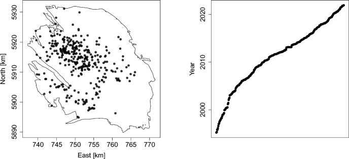 Figure 1
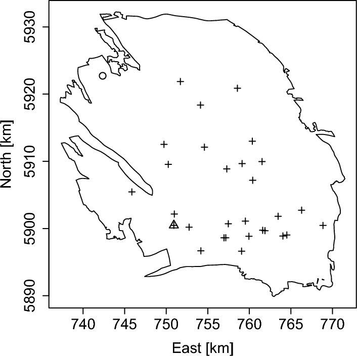 Figure 2
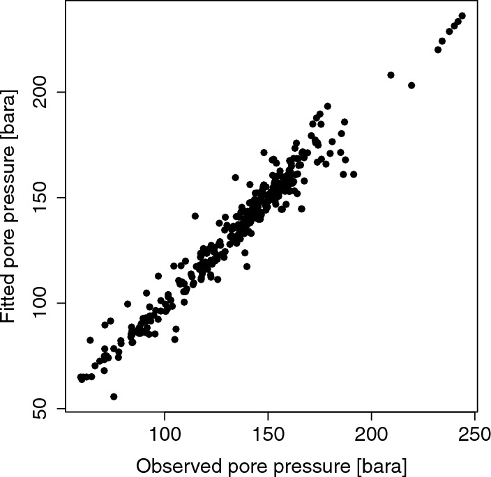 Figure 3
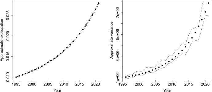 Figure 4
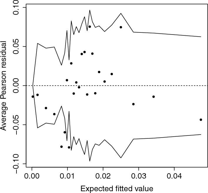 Figure 5
 Figure 6
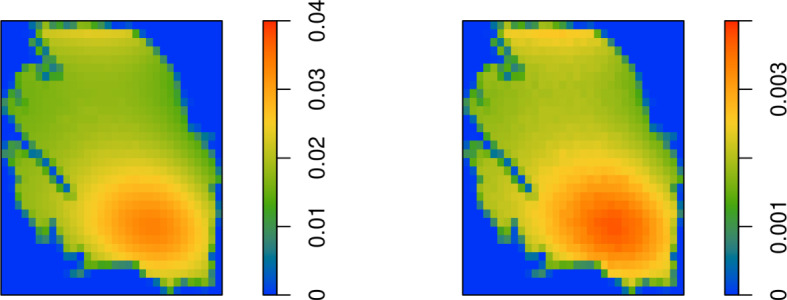 Figure 7
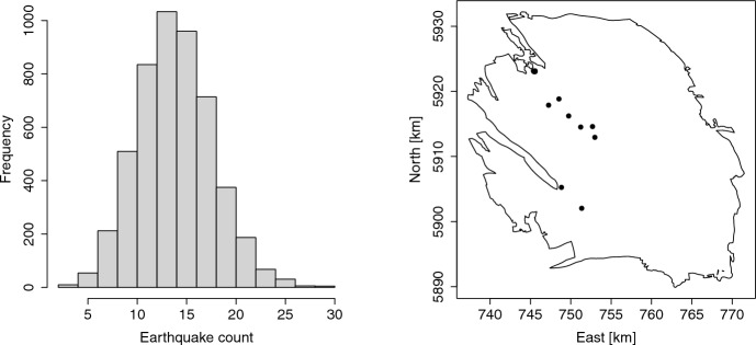 Figure 8
- —http://dx.doi.org/10.13039/501100003246Nederlandse Organisatie voor Wetenschappelijk Onderzoek
Peer Reviews
No public reviews on file for this paper yet. If you reviewed it on a platform where reviews are public (OpenReview, ICLR, NeurIPS, ICML), you can paste yours below so the community can read it here.
Videos
No videos yet. Explain this paper in a talk, walkthrough, or lecture? Add one.
Taxonomy
TopicsSeismic Imaging and Inversion Techniques · earthquake and tectonic studies · Seismic Waves and Analysis
Introduction
The study of induced earthquakes caused by the extraction or injection of fluids or gases is an important research topic. In the Netherlands, the Groningen gas field, discovered in the late 1950s, has played an important role in the Dutch economy. With an estimated recoverable gas volume of over 2,900 billion normal cubic metres spread over a region of about 900 square kilometres, it is one of the largest gas fields on the planet (Jager and Visser 2017). However, large production volumes in the 1970s caused a drop in pore pressure in the gas field which resulted in induced earthquakes in the previously seismically inactive region. The severest tremor to date occurred in August 2012 and had a magnitude of 3.6. It is estimated that the maximum possible induced magnitude is around 4 (Boitz et al. 2024). Thus, it is essential to be able to predict seismic hazard based on field measurements, for instance of pore pressure or, equivalently, Coulomb stress. One of the most widely used methodologies to do so is the rate-and-state model (Candela et al. 2019; Dempsey and Suckale 2017; Richter et al. 2020), which is now considered to be the state-of-the-art technique (Kűhn et al. 2022).
In the rate-and-state model, the earthquakes follow a Poisson point process whose intensity function \documentclass[12pt]{minimal} \usepackage{amsmath} \usepackage{wasysym} \usepackage{amsfonts} \usepackage{amssymb} \usepackage{amsbsy} \usepackage{mathrsfs} \usepackage{upgreek} \setlength{\oddsidemargin}{-69pt} \begin{document}$$\lambda $$\end{document} (the rate) is assumed to be inversely proportional to a state variable \documentclass[12pt]{minimal} \usepackage{amsmath} \usepackage{wasysym} \usepackage{amsfonts} \usepackage{amssymb} \usepackage{amsbsy} \usepackage{mathrsfs} \usepackage{upgreek} \setlength{\oddsidemargin}{-69pt} \begin{document}$$\varGamma $$\end{document} that is defined by an ordinary differential equation. This differential equation is based on physical considerations and takes into account the elapsed time and the change in pore pressure. Nevertheless, it can be criticised on several points. Firstly, since, by definition, the points in any Poisson point process do not interact with one another, the model is unable to deal with clustering as seen in, for instance, the Groningen data (Lieshout and Baki 2024). Secondly, the pressure values are assumed to be known everywhere. Lastly, the varying gas extraction is not taken into account. To address these shortcomings, in this paper, a doubly stochastic or Cox rate-and-state model is proposed. Additionally, a toolbox for statistical inference is developed.
The plan is as follows. First, Sect. 2 describes the data and reviews the Poisson rate-and-state model. Section 3 proposes a modified Cox rate-and-state model. Explicit expressions for the first and second moments of the state variable are given in Sect. 4 and, in Sect. 5, the delta method is applied to approximate the first two moments of the rate variable. Section 6 turns to the estimation of the model parameters. Next, Sect. 7 focuses on the random state variable. Its conditional distribution given earthquake count data is calculated and a parallel Metropolis-adjusted Langevin monitoring algorithm is applied to the Groningen data. The paper closes with a discussion and some suggestions for future research.
Data
In a previous paper, Lieshout and Baki (2024) carried out an exhaustive exploratory analysis of the Groningen earthquake data, including data collection, cleaning and smoothing. Here, the procedure is summarised briefly; the reader is referred to the previous work for full details.
The Groningen Gas Field
Fig. 1. Spatial (left-most panel) and temporal (right-most panel) representations of the 332 earthquakes of magnitude 1.5 or larger with epicentre in the Groningen gas field that occurred in the period from January 1st, 1995, up to December 31st, 2021. The spatial coordinates are in the UTM-31 system with kilometres as unit. The dates are given in years
The Royal Dutch Meteorological Office (KNMI) maintain an earthquake catalogue for the Netherlands (KNMI 2022). Here, we restrict attention to those tremors that occur within the Groningen gas field in the north of the country. Figure 1 shows a spatial and temporal visualisation for this field of the 332 earthquakes of magnitude at least 1.5, the magnitude of completeness, in the period from January 1st, 1995, up to December 31st, 2021. Since all earthquakes occur at the same depth, a two-dimensional analysis suffices.
The left panel is based on shapefiles from the Geological Survey of the Netherlands (TNO 2022) website. The files are updated monthly and contain a polygonal approximation of the border of the field. The map that was published in April 2022 is used here. The coordinates of the field are given in the UTM system using zone 31 with metres as the spatial unit, which in this paper are rescaled to kilometres. Note that earthquakes seem to happen more often in the central and southwestern parts of the gas field.
The right panel shows the time of occurrence of each earthquake against their chronological index number. The steeper curve in the 1990s reflects the longer spell between successive earthquake occurrences; flatter pieces indicate a quicker succession of earthquakes.
To explain the observed heterogeneity, two covariates are available. Monthly gas production values from the start of preliminary exploration in February 1956 up to and including December 2021 for all 29 production wells present in the field, indicated by a cross in Fig. 2, were kindly provided to the authors.1 The production is recorded in cubic metres, which is here rescaled to billion cubic metres (Nbcm).Fig. 2. The crosses represent the locations in the UTM-31 coordinate system (in kilometres) of 29 production wells in the Groningen gas field. The one marked by a triangle is ‘Slochteren’. Also shown is an observation well at Oldorp indicated by a circle
In order to be useful as covariate information in statistical models, the raw data over space and time are smoothed by means of an adaptive kernel approach. In doing so, values are obtained for every location and time point, which can then be aggregated as desired.
Additionally, 2, 009 pore pressure observations in bara, the unit for absolute pressure, are available on the website of the Nederlandse Aardolie Maatschappij (NAM), the exploration and production company, over the period from April 1960 until November 2018 (NAM 2022). Of these, only 352 measurements fall within the time frame used in this paper. To be able to assign a pore pressure value to each spatial location and every point in time, Lieshout and Baki (2024) fitted a polynomial regression model by the least squares method to the 352 measurements whose temporal coordinates lie in 1995 or in later years. The analysis of variance (ANOVA) table, the estimated regression parameters and their \documentclass[12pt]{minimal} \usepackage{amsmath} \usepackage{wasysym} \usepackage{amsfonts} \usepackage{amssymb} \usepackage{amsbsy} \usepackage{mathrsfs} \usepackage{upgreek} \setlength{\oddsidemargin}{-69pt} \begin{document}$$95\%$$\end{document} confidence, under the assumption that the error terms are independent Gaussians with zero mean, are given in Appendix A. The variance of the noise was estimated as well, and its estimate is also provided in Appendix A. To validate the model, Fig. 3 plots the fitted pore pressure against the observed values. Since the points lie approximately on a straight line, the fit is deemed adequate.Fig. 3. Fitted pore pressure against observed values in bara from a fourth-order polynomial Gaussian regression model (Appendix A)
The Poisson Rate-and-State Model
In the classic rate-and-state model (Candela et al. 2019; Dempsey and Suckale 2017), earthquakes occur according to a spatio-temporal Poisson point process. Such a process is completely specified by an intensity function \documentclass[12pt]{minimal} \usepackage{amsmath} \usepackage{wasysym} \usepackage{amsfonts} \usepackage{amssymb} \usepackage{amsbsy} \usepackage{mathrsfs} \usepackage{upgreek} \setlength{\oddsidemargin}{-69pt} \begin{document}$$\lambda $$\end{document} that describes the probability of an event occurring at a given time and location. For sets \documentclass[12pt]{minimal} \usepackage{amsmath} \usepackage{wasysym} \usepackage{amsfonts} \usepackage{amssymb} \usepackage{amsbsy} \usepackage{mathrsfs} \usepackage{upgreek} \setlength{\oddsidemargin}{-69pt} \begin{document}$$W_S$$\end{document} in some spatial observation window and \documentclass[12pt]{minimal} \usepackage{amsmath} \usepackage{wasysym} \usepackage{amsfonts} \usepackage{amssymb} \usepackage{amsbsy} \usepackage{mathrsfs} \usepackage{upgreek} \setlength{\oddsidemargin}{-69pt} \begin{document}$$W_T$$\end{document} in a temporal domain, the probability distribution of the number of events in \documentclass[12pt]{minimal} \usepackage{amsmath} \usepackage{wasysym} \usepackage{amsfonts} \usepackage{amssymb} \usepackage{amsbsy} \usepackage{mathrsfs} \usepackage{upgreek} \setlength{\oddsidemargin}{-69pt} \begin{document}$$W_S \times W_T$$\end{document} is a Poisson with rate \documentclass[12pt]{minimal} \usepackage{amsmath} \usepackage{wasysym} \usepackage{amsfonts} \usepackage{amssymb} \usepackage{amsbsy} \usepackage{mathrsfs} \usepackage{upgreek} \setlength{\oddsidemargin}{-69pt} \begin{document}$$\int _{W_S \times W_T} \lambda (\textbf{s},t) d\textbf{s} dt$$\end{document} . Moreover, given that there are n events, these are scattered independently according to the probability density function \documentclass[12pt]{minimal} \usepackage{amsmath} \usepackage{wasysym} \usepackage{amsfonts} \usepackage{amssymb} \usepackage{amsbsy} \usepackage{mathrsfs} \usepackage{upgreek} \setlength{\oddsidemargin}{-69pt} \begin{document}$$\lambda / \int _{W_S\times W_T} \lambda (\textbf{s},t) d\textbf{s} dt$$\end{document} . Thus, there are no interactions between the events.
The rate-and-state model is defined by
\documentclass[12pt]{minimal} \usepackage{amsmath} \usepackage{wasysym} \usepackage{amsfonts} \usepackage{amssymb} \usepackage{amsbsy} \usepackage{mathrsfs} \usepackage{upgreek} \setlength{\oddsidemargin}{-69pt} \begin{document}$$\begin{aligned} \lambda (\textbf{s},t) = r_0 \frac{\varGamma (\textbf{s},t_0)}{\varGamma (\textbf{s},t)}, \quad (\textbf{s},t) \in W_S \times W_T, \end{aligned}$$\end{document}where \documentclass[12pt]{minimal} \usepackage{amsmath} \usepackage{wasysym} \usepackage{amsfonts} \usepackage{amssymb} \usepackage{amsbsy} \usepackage{mathrsfs} \usepackage{upgreek} \setlength{\oddsidemargin}{-69pt} \begin{document}$$W_S \subset {\mathbb R}^2$$\end{document} is a compact subset of the plane, \documentclass[12pt]{minimal} \usepackage{amsmath} \usepackage{wasysym} \usepackage{amsfonts} \usepackage{amssymb} \usepackage{amsbsy} \usepackage{mathrsfs} \usepackage{upgreek} \setlength{\oddsidemargin}{-69pt} \begin{document}$$W_T$$\end{document} a closed and bounded interval in \documentclass[12pt]{minimal} \usepackage{amsmath} \usepackage{wasysym} \usepackage{amsfonts} \usepackage{amssymb} \usepackage{amsbsy} \usepackage{mathrsfs} \usepackage{upgreek} \setlength{\oddsidemargin}{-69pt} \begin{document}$${\mathbb R}$$\end{document} and \documentclass[12pt]{minimal} \usepackage{amsmath} \usepackage{wasysym} \usepackage{amsfonts} \usepackage{amssymb} \usepackage{amsbsy} \usepackage{mathrsfs} \usepackage{upgreek} \setlength{\oddsidemargin}{-69pt} \begin{document}$$t_0 = \min \{t: t \in W_T \}$$\end{document} . The parameter \documentclass[12pt]{minimal} \usepackage{amsmath} \usepackage{wasysym} \usepackage{amsfonts} \usepackage{amssymb} \usepackage{amsbsy} \usepackage{mathrsfs} \usepackage{upgreek} \setlength{\oddsidemargin}{-69pt} \begin{document}$$r_0 > 0$$\end{document} is the background seismicity; the state variable \documentclass[12pt]{minimal} \usepackage{amsmath} \usepackage{wasysym} \usepackage{amsfonts} \usepackage{amssymb} \usepackage{amsbsy} \usepackage{mathrsfs} \usepackage{upgreek} \setlength{\oddsidemargin}{-69pt} \begin{document}$$\varGamma (\textbf{s},t)$$\end{document} is defined by the ordinary differential equation
\documentclass[12pt]{minimal} \usepackage{amsmath} \usepackage{wasysym} \usepackage{amsfonts} \usepackage{amssymb} \usepackage{amsbsy} \usepackage{mathrsfs} \usepackage{upgreek} \setlength{\oddsidemargin}{-69pt} \begin{document}$$\begin{aligned} d\varGamma (\textbf{s},t) = \alpha \left( dt + \varGamma (\textbf{s},t) dX(\textbf{s},t) \right) , \end{aligned}$$\end{document}where \documentclass[12pt]{minimal} \usepackage{amsmath} \usepackage{wasysym} \usepackage{amsfonts} \usepackage{amssymb} \usepackage{amsbsy} \usepackage{mathrsfs} \usepackage{upgreek} \setlength{\oddsidemargin}{-69pt} \begin{document}$$\alpha > 0$$\end{document} is a model parameter and \documentclass[12pt]{minimal} \usepackage{amsmath} \usepackage{wasysym} \usepackage{amsfonts} \usepackage{amssymb} \usepackage{amsbsy} \usepackage{mathrsfs} \usepackage{upgreek} \setlength{\oddsidemargin}{-69pt} \begin{document}$$X(\textbf{s},t)$$\end{document} is the pore pressure at spatial location \documentclass[12pt]{minimal} \usepackage{amsmath} \usepackage{wasysym} \usepackage{amsfonts} \usepackage{amssymb} \usepackage{amsbsy} \usepackage{mathrsfs} \usepackage{upgreek} \setlength{\oddsidemargin}{-69pt} \begin{document}$$\textbf{s}$$\end{document} and time t. In the classic model, \documentclass[12pt]{minimal} \usepackage{amsmath} \usepackage{wasysym} \usepackage{amsfonts} \usepackage{amssymb} \usepackage{amsbsy} \usepackage{mathrsfs} \usepackage{upgreek} \setlength{\oddsidemargin}{-69pt} \begin{document}$$X: W_S\times W_T \rightarrow {\mathbb R}^+$$\end{document} is a deterministic function. Note that when the pore pressure remains constant, the state variable increases over time and the earthquake hazard decreases according to Omori’s law (Utsu et al. 1995). When the pore pressure changes due to gas extraction or fluid injection, an increase in pore pressure due to fluid injection emphasises the temporal increase in the state variable and thus reduces the seismic hazard even more. A drop in pore pressure contributes a negative term to Eq. (2); its effect on the intensity of earthquakes also depends on the temporal term.
Multiplying both sides of Eq. (2) by \documentclass[12pt]{minimal} \usepackage{amsmath} \usepackage{wasysym} \usepackage{amsfonts} \usepackage{amssymb} \usepackage{amsbsy} \usepackage{mathrsfs} \usepackage{upgreek} \setlength{\oddsidemargin}{-69pt} \begin{document}$$\exp ( -\alpha X(\textbf{s},t) )$$\end{document} , discretising in time steps of length \documentclass[12pt]{minimal} \usepackage{amsmath} \usepackage{wasysym} \usepackage{amsfonts} \usepackage{amssymb} \usepackage{amsbsy} \usepackage{mathrsfs} \usepackage{upgreek} \setlength{\oddsidemargin}{-69pt} \begin{document}$$\varDelta > 0$$\end{document} and writing \documentclass[12pt]{minimal} \usepackage{amsmath} \usepackage{wasysym} \usepackage{amsfonts} \usepackage{amssymb} \usepackage{amsbsy} \usepackage{mathrsfs} \usepackage{upgreek} \setlength{\oddsidemargin}{-69pt} \begin{document}$$t_k = t_0 + k\varDelta $$\end{document} , \documentclass[12pt]{minimal} \usepackage{amsmath} \usepackage{wasysym} \usepackage{amsfonts} \usepackage{amssymb} \usepackage{amsbsy} \usepackage{mathrsfs} \usepackage{upgreek} \setlength{\oddsidemargin}{-69pt} \begin{document}$$k=1, \dots , m$$\end{document} , one obtains the Euler difference equation
\documentclass[12pt]{minimal} \usepackage{amsmath} \usepackage{wasysym} \usepackage{amsfonts} \usepackage{amssymb} \usepackage{amsbsy} \usepackage{mathrsfs} \usepackage{upgreek} \setlength{\oddsidemargin}{-69pt} \begin{document}$$\begin{aligned} \varGamma (\textbf{s}, t_{k +1} ) = \left( \varGamma (\textbf{s}, t_k) + \alpha \varDelta \right) \exp \left( \alpha ( X(\textbf{s},t_{k+1} ) - X(\textbf{s},t_k) ) \right) , \quad \textbf{s} \in W_S. \end{aligned}$$\end{document}The parameters \documentclass[12pt]{minimal} \usepackage{amsmath} \usepackage{wasysym} \usepackage{amsfonts} \usepackage{amssymb} \usepackage{amsbsy} \usepackage{mathrsfs} \usepackage{upgreek} \setlength{\oddsidemargin}{-69pt} \begin{document}$$r_0$$\end{document} , \documentclass[12pt]{minimal} \usepackage{amsmath} \usepackage{wasysym} \usepackage{amsfonts} \usepackage{amssymb} \usepackage{amsbsy} \usepackage{mathrsfs} \usepackage{upgreek} \setlength{\oddsidemargin}{-69pt} \begin{document}$$\alpha $$\end{document} and the initial state \documentclass[12pt]{minimal} \usepackage{amsmath} \usepackage{wasysym} \usepackage{amsfonts} \usepackage{amssymb} \usepackage{amsbsy} \usepackage{mathrsfs} \usepackage{upgreek} \setlength{\oddsidemargin}{-69pt} \begin{document}$$\varGamma (\textbf{s}, t_0) \equiv \gamma _0 > 0$$\end{document} are treated as unknowns and can be estimated, for example, by the maximum likelihood method. For a full discussion and comparison with other techniques, see Kűhn et al. (2022). In line with current practice, the spatial domain \documentclass[12pt]{minimal} \usepackage{amsmath} \usepackage{wasysym} \usepackage{amsfonts} \usepackage{amssymb} \usepackage{amsbsy} \usepackage{mathrsfs} \usepackage{upgreek} \setlength{\oddsidemargin}{-69pt} \begin{document}$$W_S$$\end{document} is discretised in a regular grid with cell representatives \documentclass[12pt]{minimal} \usepackage{amsmath} \usepackage{wasysym} \usepackage{amsfonts} \usepackage{amssymb} \usepackage{amsbsy} \usepackage{mathrsfs} \usepackage{upgreek} \setlength{\oddsidemargin}{-69pt} \begin{document}$$\textbf{s}_1, \dots , \textbf{s}_n$$\end{document} . Note that because \documentclass[12pt]{minimal} \usepackage{amsmath} \usepackage{wasysym} \usepackage{amsfonts} \usepackage{amssymb} \usepackage{amsbsy} \usepackage{mathrsfs} \usepackage{upgreek} \setlength{\oddsidemargin}{-69pt} \begin{document}$$W_S$$\end{document} is not necessarily rectangular, grid cells may have different areas, which are denoted by \documentclass[12pt]{minimal} \usepackage{amsmath} \usepackage{wasysym} \usepackage{amsfonts} \usepackage{amssymb} \usepackage{amsbsy} \usepackage{mathrsfs} \usepackage{upgreek} \setlength{\oddsidemargin}{-69pt} \begin{document}$$\varDelta (\textbf{s}_i)$$\end{document} . For our data, take \documentclass[12pt]{minimal} \usepackage{amsmath} \usepackage{wasysym} \usepackage{amsfonts} \usepackage{amssymb} \usepackage{amsbsy} \usepackage{mathrsfs} \usepackage{upgreek} \setlength{\oddsidemargin}{-69pt} \begin{document}$$\varDelta $$\end{document} equal to 1 year and partition \documentclass[12pt]{minimal} \usepackage{amsmath} \usepackage{wasysym} \usepackage{amsfonts} \usepackage{amssymb} \usepackage{amsbsy} \usepackage{mathrsfs} \usepackage{upgreek} \setlength{\oddsidemargin}{-69pt} \begin{document}$$W_S$$\end{document} in a 32 by 32 grid.
The model defined by Eq. (1), Eq. (2) and Eq. (3) has several shortcomings. First of all, of the two covariates at our disposal, only one is used. Secondly, an exploratory analysis in Lieshout and Baki (2024) indicated that the data exhibit clustering that cannot be accounted for by the Poisson model. Finally, the variance of the regression model for the pore pressure is ignored, but should be taken into account given the sparsity of observations. In the next section, the rate-and-state model will be modified so that these issues are resolved.
The Cox Rate-and-State Model
The Poisson rate-and-state model discussed in Sect. 2.2 expresses the change in seismic hazard in terms of elapsed time and pore pressure change. In practice, the values of the latter are typically available only at wells and monitoring stations. At other locations, the pore pressure must be estimated (Lieshout and Baki 2024) or approximated by linear (or spline-based) interpolation (Richter et al. 2020). For the Groningen data described in Sect. 2, there are only about 2,000 observations scattered unevenly over the field and spanning a period of several decades. Therefore, it would be better to explicitly take the uncertainty into account and treat the \documentclass[12pt]{minimal} \usepackage{amsmath} \usepackage{wasysym} \usepackage{amsfonts} \usepackage{amssymb} \usepackage{amsbsy} \usepackage{mathrsfs} \usepackage{upgreek} \setlength{\oddsidemargin}{-69pt} \begin{document}$$X(\textbf{s}_i, t_j)$$\end{document} as random variables. By doing so, one obtains a doubly stochastic or Cox point process (Chiu et al. 2013). Briefly, given a realisation \documentclass[12pt]{minimal} \usepackage{amsmath} \usepackage{wasysym} \usepackage{amsfonts} \usepackage{amssymb} \usepackage{amsbsy} \usepackage{mathrsfs} \usepackage{upgreek} \setlength{\oddsidemargin}{-69pt} \begin{document}$$\lambda $$\end{document} of the density \documentclass[12pt]{minimal} \usepackage{amsmath} \usepackage{wasysym} \usepackage{amsfonts} \usepackage{amssymb} \usepackage{amsbsy} \usepackage{mathrsfs} \usepackage{upgreek} \setlength{\oddsidemargin}{-69pt} \begin{document}$$\varLambda $$\end{document} of a random measure on \documentclass[12pt]{minimal} \usepackage{amsmath} \usepackage{wasysym} \usepackage{amsfonts} \usepackage{amssymb} \usepackage{amsbsy} \usepackage{mathrsfs} \usepackage{upgreek} \setlength{\oddsidemargin}{-69pt} \begin{document}$$W_S\times W_T$$\end{document} , the driving random measure of the Cox process, the earthquakes form a Poisson point process with intensity function \documentclass[12pt]{minimal} \usepackage{amsmath} \usepackage{wasysym} \usepackage{amsfonts} \usepackage{amssymb} \usepackage{amsbsy} \usepackage{mathrsfs} \usepackage{upgreek} \setlength{\oddsidemargin}{-69pt} \begin{document}$$\lambda $$\end{document} . Thus, the distribution of the Cox process is fully characterised by the distribution of the driving random measure.
To find a suitable driving random measure, assume that the pore pressure can be decomposed into a deterministic and stochastic part, that is,
\documentclass[12pt]{minimal} \usepackage{amsmath} \usepackage{wasysym} \usepackage{amsfonts} \usepackage{amssymb} \usepackage{amsbsy} \usepackage{mathrsfs} \usepackage{upgreek} \setlength{\oddsidemargin}{-69pt} \begin{document}$$\begin{aligned} X(\textbf{s}_i, t_j) = m(\textbf{s}_i, t_j) + E(\textbf{s}_i, t_j). \end{aligned}$$\end{document}Here \documentclass[12pt]{minimal} \usepackage{amsmath} \usepackage{wasysym} \usepackage{amsfonts} \usepackage{amssymb} \usepackage{amsbsy} \usepackage{mathrsfs} \usepackage{upgreek} \setlength{\oddsidemargin}{-69pt} \begin{document}$$E(\textbf{s}_i,t_j)$$\end{document} are independent mean-zero random variables with variance \documentclass[12pt]{minimal} \usepackage{amsmath} \usepackage{wasysym} \usepackage{amsfonts} \usepackage{amssymb} \usepackage{amsbsy} \usepackage{mathrsfs} \usepackage{upgreek} \setlength{\oddsidemargin}{-69pt} \begin{document}$$\sigma ^2$$\end{document} and m is the fitted polynomial regression model described in Sect. 2 and Appendix A. Since the variogram of the residuals is flat in time (Lieshout and Baki 2024), the residual variation is a function of spatial location only, which, since the rate-state equation (cf. Eq. (2)) depends only on temporal changes in pore pressure, may be ignored.
The random variables \documentclass[12pt]{minimal} \usepackage{amsmath} \usepackage{wasysym} \usepackage{amsfonts} \usepackage{amssymb} \usepackage{amsbsy} \usepackage{mathrsfs} \usepackage{upgreek} \setlength{\oddsidemargin}{-69pt} \begin{document}$$X(\textbf{s}_i, t_j)$$\end{document} are then plugged into the Euler difference equation (cf. Eq. (3)), and upon solving for the random variable \documentclass[12pt]{minimal} \usepackage{amsmath} \usepackage{wasysym} \usepackage{amsfonts} \usepackage{amssymb} \usepackage{amsbsy} \usepackage{mathrsfs} \usepackage{upgreek} \setlength{\oddsidemargin}{-69pt} \begin{document}$$\varGamma (\textbf{s}_i, t_j)$$\end{document} , one obtains
\documentclass[12pt]{minimal} \usepackage{amsmath} \usepackage{wasysym} \usepackage{amsfonts} \usepackage{amssymb} \usepackage{amsbsy} \usepackage{mathrsfs} \usepackage{upgreek} \setlength{\oddsidemargin}{-69pt} \begin{document}$$\begin{aligned} \varGamma (\textbf{s}_i, t_j) = \exp \left( \alpha X(\textbf{s}_i, t_j) \right) \left\{ \alpha \varDelta \sum _{k=0}^{j-1} \exp \left( - \alpha X(\textbf{s}_i, t_k) \right) + \gamma _0 \exp \left( - \alpha X(\textbf{s}_i, t_0) \right) \right\} . \end{aligned}$$\end{document}The interpretation of the parameter \documentclass[12pt]{minimal} \usepackage{amsmath} \usepackage{wasysym} \usepackage{amsfonts} \usepackage{amssymb} \usepackage{amsbsy} \usepackage{mathrsfs} \usepackage{upgreek} \setlength{\oddsidemargin}{-69pt} \begin{document}$$\alpha $$\end{document} is the same as for the original rate-and-state model. In particular, when the pore pressure decreases as a consequence of gas extraction, \documentclass[12pt]{minimal} \usepackage{amsmath} \usepackage{wasysym} \usepackage{amsfonts} \usepackage{amssymb} \usepackage{amsbsy} \usepackage{mathrsfs} \usepackage{upgreek} \setlength{\oddsidemargin}{-69pt} \begin{document}$$\alpha $$\end{document} must be positive. As for the classic model, \documentclass[12pt]{minimal} \usepackage{amsmath} \usepackage{wasysym} \usepackage{amsfonts} \usepackage{amssymb} \usepackage{amsbsy} \usepackage{mathrsfs} \usepackage{upgreek} \setlength{\oddsidemargin}{-69pt} \begin{document}$$\gamma _0>0$$\end{document} is the initial state of the stochastic difference equation.
The other explanatory variable at our disposal is the vector of smoothed gas production (cf. Sect. 2). Its influence on the earthquake intensity function can be modelled through the multiplier \documentclass[12pt]{minimal} \usepackage{amsmath} \usepackage{wasysym} \usepackage{amsfonts} \usepackage{amssymb} \usepackage{amsbsy} \usepackage{mathrsfs} \usepackage{upgreek} \setlength{\oddsidemargin}{-69pt} \begin{document}$$r_0$$\end{document} in Eq. (1). Specifically, set \documentclass[12pt]{minimal} \usepackage{amsmath} \usepackage{wasysym} \usepackage{amsfonts} \usepackage{amssymb} \usepackage{amsbsy} \usepackage{mathrsfs} \usepackage{upgreek} \setlength{\oddsidemargin}{-69pt} \begin{document}$$\varDelta $$\end{document} equal to 1 year. This choice of \documentclass[12pt]{minimal} \usepackage{amsmath} \usepackage{wasysym} \usepackage{amsfonts} \usepackage{amssymb} \usepackage{amsbsy} \usepackage{mathrsfs} \usepackage{upgreek} \setlength{\oddsidemargin}{-69pt} \begin{document}$$\varDelta $$\end{document} is convenient, as it implies that there is no need to account for seasonal fluctuations. Also, write \documentclass[12pt]{minimal} \usepackage{amsmath} \usepackage{wasysym} \usepackage{amsfonts} \usepackage{amssymb} \usepackage{amsbsy} \usepackage{mathrsfs} \usepackage{upgreek} \setlength{\oddsidemargin}{-69pt} \begin{document}$$V(\textbf{s}_i, t_j)$$\end{document} for the volume of gas extracted in the grid cell around \documentclass[12pt]{minimal} \usepackage{amsmath} \usepackage{wasysym} \usepackage{amsfonts} \usepackage{amssymb} \usepackage{amsbsy} \usepackage{mathrsfs} \usepackage{upgreek} \setlength{\oddsidemargin}{-69pt} \begin{document}$$\textbf{s}_i \in W_S$$\end{document} over the year preceding \documentclass[12pt]{minimal} \usepackage{amsmath} \usepackage{wasysym} \usepackage{amsfonts} \usepackage{amssymb} \usepackage{amsbsy} \usepackage{mathrsfs} \usepackage{upgreek} \setlength{\oddsidemargin}{-69pt} \begin{document}$$t_j$$\end{document} . The idea is then to replace the constant \documentclass[12pt]{minimal} \usepackage{amsmath} \usepackage{wasysym} \usepackage{amsfonts} \usepackage{amssymb} \usepackage{amsbsy} \usepackage{mathrsfs} \usepackage{upgreek} \setlength{\oddsidemargin}{-69pt} \begin{document}$$r_0$$\end{document} by \documentclass[12pt]{minimal} \usepackage{amsmath} \usepackage{wasysym} \usepackage{amsfonts} \usepackage{amssymb} \usepackage{amsbsy} \usepackage{mathrsfs} \usepackage{upgreek} \setlength{\oddsidemargin}{-69pt} \begin{document}$$\exp \left( \theta _1 + \theta _2 V(\textbf{s}_i, t_j) \right) $$\end{document} . The real-valued parameter \documentclass[12pt]{minimal} \usepackage{amsmath} \usepackage{wasysym} \usepackage{amsfonts} \usepackage{amssymb} \usepackage{amsbsy} \usepackage{mathrsfs} \usepackage{upgreek} \setlength{\oddsidemargin}{-69pt} \begin{document}$$\theta _1$$\end{document} is the intercept and the parameter \documentclass[12pt]{minimal} \usepackage{amsmath} \usepackage{wasysym} \usepackage{amsfonts} \usepackage{amssymb} \usepackage{amsbsy} \usepackage{mathrsfs} \usepackage{upgreek} \setlength{\oddsidemargin}{-69pt} \begin{document}$$\theta _2$$\end{document} quantifies the effect of gas extraction. For positive \documentclass[12pt]{minimal} \usepackage{amsmath} \usepackage{wasysym} \usepackage{amsfonts} \usepackage{amssymb} \usepackage{amsbsy} \usepackage{mathrsfs} \usepackage{upgreek} \setlength{\oddsidemargin}{-69pt} \begin{document}$$\theta _2$$\end{document} , an increase in production tends to increase the number of earthquakes. Mathematically, the model is well-defined for \documentclass[12pt]{minimal} \usepackage{amsmath} \usepackage{wasysym} \usepackage{amsfonts} \usepackage{amssymb} \usepackage{amsbsy} \usepackage{mathrsfs} \usepackage{upgreek} \setlength{\oddsidemargin}{-69pt} \begin{document}$$\theta _2 \le 0$$\end{document} as well, but does not make practical sense.
In summary, one obtains a Cox process \documentclass[12pt]{minimal} \usepackage{amsmath} \usepackage{wasysym} \usepackage{amsfonts} \usepackage{amssymb} \usepackage{amsbsy} \usepackage{mathrsfs} \usepackage{upgreek} \setlength{\oddsidemargin}{-69pt} \begin{document}$$\varPsi $$\end{document} with driving random measure defined by its density function
\documentclass[12pt]{minimal} \usepackage{amsmath} \usepackage{wasysym} \usepackage{amsfonts} \usepackage{amssymb} \usepackage{amsbsy} \usepackage{mathrsfs} \usepackage{upgreek} \setlength{\oddsidemargin}{-69pt} \begin{document}$$\begin{aligned} \varLambda (\textbf{s}_i,t_j) = \exp \left( \theta _1 + \theta _2 V(\textbf{s}_i,t_j) \right) \frac{ \gamma _0}{ \varGamma (\textbf{s}_i,t_j)}. \end{aligned}$$\end{document}Thus, writing \documentclass[12pt]{minimal} \usepackage{amsmath} \usepackage{wasysym} \usepackage{amsfonts} \usepackage{amssymb} \usepackage{amsbsy} \usepackage{mathrsfs} \usepackage{upgreek} \setlength{\oddsidemargin}{-69pt} \begin{document}$$N(\textbf{s}_i,t_j)$$\end{document} for the number of earthquakes in the space-time cell defined by \documentclass[12pt]{minimal} \usepackage{amsmath} \usepackage{wasysym} \usepackage{amsfonts} \usepackage{amssymb} \usepackage{amsbsy} \usepackage{mathrsfs} \usepackage{upgreek} \setlength{\oddsidemargin}{-69pt} \begin{document}$$\textbf{s}_i$$\end{document} and \documentclass[12pt]{minimal} \usepackage{amsmath} \usepackage{wasysym} \usepackage{amsfonts} \usepackage{amssymb} \usepackage{amsbsy} \usepackage{mathrsfs} \usepackage{upgreek} \setlength{\oddsidemargin}{-69pt} \begin{document}$$t_j$$\end{document} , conditional on \documentclass[12pt]{minimal} \usepackage{amsmath} \usepackage{wasysym} \usepackage{amsfonts} \usepackage{amssymb} \usepackage{amsbsy} \usepackage{mathrsfs} \usepackage{upgreek} \setlength{\oddsidemargin}{-69pt} \begin{document}$$\varLambda (\textbf{s}_i, t_j)$$\end{document} , \documentclass[12pt]{minimal} \usepackage{amsmath} \usepackage{wasysym} \usepackage{amsfonts} \usepackage{amssymb} \usepackage{amsbsy} \usepackage{mathrsfs} \usepackage{upgreek} \setlength{\oddsidemargin}{-69pt} \begin{document}$$N(\textbf{s}_i, t_j)$$\end{document} is Poisson distributed with rate parameter \documentclass[12pt]{minimal} \usepackage{amsmath} \usepackage{wasysym} \usepackage{amsfonts} \usepackage{amssymb} \usepackage{amsbsy} \usepackage{mathrsfs} \usepackage{upgreek} \setlength{\oddsidemargin}{-69pt} \begin{document}$$\varLambda (\textbf{s}_i,t_j) \varDelta (\textbf{s}_i) \varDelta $$\end{document} independently of the earthquake counts in other cells. Following Richter et al. (2020), in the sequel Eq. (6) will be re-parametrised in terms of \documentclass[12pt]{minimal} \usepackage{amsmath} \usepackage{wasysym} \usepackage{amsfonts} \usepackage{amssymb} \usepackage{amsbsy} \usepackage{mathrsfs} \usepackage{upgreek} \setlength{\oddsidemargin}{-69pt} \begin{document}$$\alpha $$\end{document} , \documentclass[12pt]{minimal} \usepackage{amsmath} \usepackage{wasysym} \usepackage{amsfonts} \usepackage{amssymb} \usepackage{amsbsy} \usepackage{mathrsfs} \usepackage{upgreek} \setlength{\oddsidemargin}{-69pt} \begin{document}$$\theta _1$$\end{document} , \documentclass[12pt]{minimal} \usepackage{amsmath} \usepackage{wasysym} \usepackage{amsfonts} \usepackage{amssymb} \usepackage{amsbsy} \usepackage{mathrsfs} \usepackage{upgreek} \setlength{\oddsidemargin}{-69pt} \begin{document}$$\theta _2$$\end{document} and \documentclass[12pt]{minimal} \usepackage{amsmath} \usepackage{wasysym} \usepackage{amsfonts} \usepackage{amssymb} \usepackage{amsbsy} \usepackage{mathrsfs} \usepackage{upgreek} \setlength{\oddsidemargin}{-69pt} \begin{document}$$\eta = \log (\alpha /\gamma _0)$$\end{document} .
The Cox model defined by Eq. (6) achieves the set goals: it incorporates both available covariates, accounts for the uncertainty in the pore pressure interpolation, and exhibits clustering in time within grid cells. The latter statement follows from the fact that the pair correlation function of the proposed Cox model is greater than 1, that is,
\documentclass[12pt]{minimal} \usepackage{amsmath} \usepackage{wasysym} \usepackage{amsfonts} \usepackage{amssymb} \usepackage{amsbsy} \usepackage{mathrsfs} \usepackage{upgreek} \setlength{\oddsidemargin}{-69pt} \begin{document}$$\begin{aligned} g( (\textbf{s}_i, t_j), (\textbf{s}_i, t_k) ) = e^{\alpha ^2\sigma ^2} \ge 1, \quad 0< t_j < t_k. \end{aligned}$$\end{document}Note that the greater the uncertainty, the stronger the clustering.
Moments of the State Variable
Since the randomness in the driving random measure (cf. Eq. (6)) of our Cox process is induced by the state process \documentclass[12pt]{minimal} \usepackage{amsmath} \usepackage{wasysym} \usepackage{amsfonts} \usepackage{amssymb} \usepackage{amsbsy} \usepackage{mathrsfs} \usepackage{upgreek} \setlength{\oddsidemargin}{-69pt} \begin{document}$$\varGamma $$\end{document} through the error term E in Eq. (4), the first and second-moment properties of \documentclass[12pt]{minimal} \usepackage{amsmath} \usepackage{wasysym} \usepackage{amsfonts} \usepackage{amssymb} \usepackage{amsbsy} \usepackage{mathrsfs} \usepackage{upgreek} \setlength{\oddsidemargin}{-69pt} \begin{document}$$\varGamma $$\end{document} are investigated first.
Let \documentclass[12pt]{minimal} \usepackage{amsmath} \usepackage{wasysym} \usepackage{amsfonts} \usepackage{amssymb} \usepackage{amsbsy} \usepackage{mathrsfs} \usepackage{upgreek} \setlength{\oddsidemargin}{-69pt} \begin{document}$$\varGamma $$\end{document} be defined by Eq. (5) for some \documentclass[12pt]{minimal} \usepackage{amsmath} \usepackage{wasysym} \usepackage{amsfonts} \usepackage{amssymb} \usepackage{amsbsy} \usepackage{mathrsfs} \usepackage{upgreek} \setlength{\oddsidemargin}{-69pt} \begin{document}$$\textbf{s}\in W_S$$\end{document} and \documentclass[12pt]{minimal} \usepackage{amsmath} \usepackage{wasysym} \usepackage{amsfonts} \usepackage{amssymb} \usepackage{amsbsy} \usepackage{mathrsfs} \usepackage{upgreek} \setlength{\oddsidemargin}{-69pt} \begin{document}$$t_j$$\end{document} , \documentclass[12pt]{minimal} \usepackage{amsmath} \usepackage{wasysym} \usepackage{amsfonts} \usepackage{amssymb} \usepackage{amsbsy} \usepackage{mathrsfs} \usepackage{upgreek} \setlength{\oddsidemargin}{-69pt} \begin{document}$$j=0,\dots , m$$\end{document} . Set \documentclass[12pt]{minimal} \usepackage{amsmath} \usepackage{wasysym} \usepackage{amsfonts} \usepackage{amssymb} \usepackage{amsbsy} \usepackage{mathrsfs} \usepackage{upgreek} \setlength{\oddsidemargin}{-69pt} \begin{document}$$d = \exp \left( \alpha ^2 \sigma ^2\right) $$\end{document} and define, for \documentclass[12pt]{minimal} \usepackage{amsmath} \usepackage{wasysym} \usepackage{amsfonts} \usepackage{amssymb} \usepackage{amsbsy} \usepackage{mathrsfs} \usepackage{upgreek} \setlength{\oddsidemargin}{-69pt} \begin{document}$$i,j \in \{ 0, \dots , m \}$$\end{document} , \documentclass[12pt]{minimal} \usepackage{amsmath} \usepackage{wasysym} \usepackage{amsfonts} \usepackage{amssymb} \usepackage{amsbsy} \usepackage{mathrsfs} \usepackage{upgreek} \setlength{\oddsidemargin}{-69pt} \begin{document}$$ f_{ij} = \exp \left( \alpha \left\{ m(\textbf{s}, t_i) - m(\textbf{s}, t_j) \right\} \right) . $$\end{document} Then, for \documentclass[12pt]{minimal} \usepackage{amsmath} \usepackage{wasysym} \usepackage{amsfonts} \usepackage{amssymb} \usepackage{amsbsy} \usepackage{mathrsfs} \usepackage{upgreek} \setlength{\oddsidemargin}{-69pt} \begin{document}$$k = 1, \dots , m$$\end{document} ,
\documentclass[12pt]{minimal} \usepackage{amsmath} \usepackage{wasysym} \usepackage{amsfonts} \usepackage{amssymb} \usepackage{amsbsy} \usepackage{mathrsfs} \usepackage{upgreek} \setlength{\oddsidemargin}{-69pt} \begin{document}$$\begin{aligned} {\mathbb E}\left[ \varGamma (\textbf{s}, t_k)\right]= & d \alpha \left( \varDelta \sum _{i=0}^{k-1} f_{ki} + e^{-\eta } f_{k0} \right) ,\\ \mathrm{{Var}}\left[ \varGamma (\textbf{s}, t_k) \right]= & \alpha ^2 \varDelta ^2 d^2 (d^2 - 1) \sum _{i=0}^{k-1} f_{ki}^2 + \alpha ^2 \varDelta ^2 d^2 (d-1) \sum _{i=0}^{k-1} \sum _{i\ne j=0}^{k-1} f_{ki} f_{kj} \\ & + 2 \alpha ^2 e^{-\eta } \varDelta d^2 f_{k0}^2 \left( d^2 - 1 + (d-1) \sum _{i=1}^{k-1} f_{0i} \right) \\ & + \alpha ^2 e^{-2\eta } f_{k0}^2 d^2 (d^2 - 1), \end{aligned}$$\end{document}and, for \documentclass[12pt]{minimal} \usepackage{amsmath} \usepackage{wasysym} \usepackage{amsfonts} \usepackage{amssymb} \usepackage{amsbsy} \usepackage{mathrsfs} \usepackage{upgreek} \setlength{\oddsidemargin}{-69pt} \begin{document}$$0< k < l \le m$$\end{document} ,
\documentclass[12pt]{minimal} \usepackage{amsmath} \usepackage{wasysym} \usepackage{amsfonts} \usepackage{amssymb} \usepackage{amsbsy} \usepackage{mathrsfs} \usepackage{upgreek} \setlength{\oddsidemargin}{-69pt} \begin{document}$$\begin{aligned} \mathrm{{Cov}}( \varGamma (\textbf{s}, t_k), \varGamma (\textbf{s}, t_l) )= & \alpha ^2 \varDelta ^2 d^2 \sum _{i=0}^{k-1} \left\{ f_{ki} f_{li} (d-1) - f_{li} \left( 1 - \frac{1}{d} \right) \right\} \nonumber \\ & + \alpha ^2 e^{-\eta } ( 2 \varDelta + e^{-\eta }) d^2 f_{k0} f_{l0} ( d - 1) \nonumber \\ & - \alpha ^2 e^{-\eta } \varDelta d^2 f_{l0} \left( 1 - \frac{1}{d} \right) . \end{aligned}$$\end{document}When fluid is injected into a field, the pore pressure typically increases. In this case, the state variables are positively correlated, that is, \documentclass[12pt]{minimal} \usepackage{amsmath} \usepackage{wasysym} \usepackage{amsfonts} \usepackage{amssymb} \usepackage{amsbsy} \usepackage{mathrsfs} \usepackage{upgreek} \setlength{\oddsidemargin}{-69pt} \begin{document}$$\mathrm{{Cov}}( \varGamma (\textbf{s}, t_k), \varGamma (\textbf{s}, t_l) ) \ge 0$$\end{document} for all k, l. When the pore pressure decreases, for example, due to gas extraction, the picture is more varied. If \documentclass[12pt]{minimal} \usepackage{amsmath} \usepackage{wasysym} \usepackage{amsfonts} \usepackage{amssymb} \usepackage{amsbsy} \usepackage{mathrsfs} \usepackage{upgreek} \setlength{\oddsidemargin}{-69pt} \begin{document}$$ \alpha \sigma ^2 > m(\textbf{s}, t_0)$$\end{document} , then \documentclass[12pt]{minimal} \usepackage{amsmath} \usepackage{wasysym} \usepackage{amsfonts} \usepackage{amssymb} \usepackage{amsbsy} \usepackage{mathrsfs} \usepackage{upgreek} \setlength{\oddsidemargin}{-69pt} \begin{document}$$\mathrm{{Cov}}( \varGamma (\textbf{s}, t_k), \varGamma (\textbf{s}, t_l) ) \ge 0$$\end{document} for all k, l. On the other hand, if \documentclass[12pt]{minimal} \usepackage{amsmath} \usepackage{wasysym} \usepackage{amsfonts} \usepackage{amssymb} \usepackage{amsbsy} \usepackage{mathrsfs} \usepackage{upgreek} \setlength{\oddsidemargin}{-69pt} \begin{document}$$ \alpha \sigma ^2 < \min _{i = 0, \dots , m-1} \left\{ m(\textbf{s}, t_i) - m(\textbf{s}, t_{i+1}) \right\} , $$\end{document} the minimal drop in pressure in between observation epochs, for all \documentclass[12pt]{minimal} \usepackage{amsmath} \usepackage{wasysym} \usepackage{amsfonts} \usepackage{amssymb} \usepackage{amsbsy} \usepackage{mathrsfs} \usepackage{upgreek} \setlength{\oddsidemargin}{-69pt} \begin{document}$$0 \le k < l \le m$$\end{document} ,
\documentclass[12pt]{minimal} \usepackage{amsmath} \usepackage{wasysym} \usepackage{amsfonts} \usepackage{amssymb} \usepackage{amsbsy} \usepackage{mathrsfs} \usepackage{upgreek} \setlength{\oddsidemargin}{-69pt} \begin{document}$$\begin{aligned} \mathrm{{Cov}}( \varGamma (\textbf{s}, t_k), \varGamma (s, t_l) ) - \alpha ^2 e^{-\eta } ( \varDelta + e^{-\eta } ) d^2 (d-1) f_{k0} f_{l0} \le 0. \end{aligned}$$\end{document}The proofs of these statements can be found in Appendix B. The following examples are illuminating.Table 1. Estimated pore pressure in bara on January 1st in the years 1995–2021 near the town of Slochteren (UTM-31 coordinates (750, 5900) in kilometres), The NetherlandsYears1995–2001179.81177.39174.86172.20169.42166.50163.482002–2008160.32157.05153.65150.13146.49142.72138.822009–2015134.81130.68126.43122.04117.53112.91108.162016–2021103.2898.2993.1787.9482.5677.08
Example 1
Table 1 lists estimated pore pressure values near the town of Slochteren, indicated by a triangle in Fig. 2, in the Groningen gas field in the Netherlands for January 1st, 1995–2021 (Lieshout and Baki 2024). Specifically, the first entry in the top row, 179.81 bara, corresponds to the year 1995, the second entry to 1996 and so on.
Note that the pore pressure values are decreasing due to gas extraction. Since the intensity of induced earthquakes was very low in 1995, \documentclass[12pt]{minimal} \usepackage{amsmath} \usepackage{wasysym} \usepackage{amsfonts} \usepackage{amssymb} \usepackage{amsbsy} \usepackage{mathrsfs} \usepackage{upgreek} \setlength{\oddsidemargin}{-69pt} \begin{document}$$\gamma _0$$\end{document} can be considered infinite. Hence \documentclass[12pt]{minimal} \usepackage{amsmath} \usepackage{wasysym} \usepackage{amsfonts} \usepackage{amssymb} \usepackage{amsbsy} \usepackage{mathrsfs} \usepackage{upgreek} \setlength{\oddsidemargin}{-69pt} \begin{document}$$\eta = -\infty $$\end{document} and Eq. (7) then implies that the covariance matrix of the random vector \documentclass[12pt]{minimal} \usepackage{amsmath} \usepackage{wasysym} \usepackage{amsfonts} \usepackage{amssymb} \usepackage{amsbsy} \usepackage{mathrsfs} \usepackage{upgreek} \setlength{\oddsidemargin}{-69pt} \begin{document}$$\varGamma (\textbf{s}, t_k)_{k=1,\dots , m}$$\end{document} has positive entries only.
Example 2
Next, suppose that – in contrast to the previous example – the initial seismicity is very high, that is, \documentclass[12pt]{minimal} \usepackage{amsmath} \usepackage{wasysym} \usepackage{amsfonts} \usepackage{amssymb} \usepackage{amsbsy} \usepackage{mathrsfs} \usepackage{upgreek} \setlength{\oddsidemargin}{-69pt} \begin{document}$$\gamma _0 = 0$$\end{document} or \documentclass[12pt]{minimal} \usepackage{amsmath} \usepackage{wasysym} \usepackage{amsfonts} \usepackage{amssymb} \usepackage{amsbsy} \usepackage{mathrsfs} \usepackage{upgreek} \setlength{\oddsidemargin}{-69pt} \begin{document}$$\eta = \infty $$\end{document} . Assume a linearly decreasing sequence of pore pressures \documentclass[12pt]{minimal} \usepackage{amsmath} \usepackage{wasysym} \usepackage{amsfonts} \usepackage{amssymb} \usepackage{amsbsy} \usepackage{mathrsfs} \usepackage{upgreek} \setlength{\oddsidemargin}{-69pt} \begin{document}$$m(\textbf{s}, 0) = 3$$\end{document} , \documentclass[12pt]{minimal} \usepackage{amsmath} \usepackage{wasysym} \usepackage{amsfonts} \usepackage{amssymb} \usepackage{amsbsy} \usepackage{mathrsfs} \usepackage{upgreek} \setlength{\oddsidemargin}{-69pt} \begin{document}$$m(\textbf{s}, 1) = 2 $$\end{document} and \documentclass[12pt]{minimal} \usepackage{amsmath} \usepackage{wasysym} \usepackage{amsfonts} \usepackage{amssymb} \usepackage{amsbsy} \usepackage{mathrsfs} \usepackage{upgreek} \setlength{\oddsidemargin}{-69pt} \begin{document}$$m(\textbf{s}, 2) = 1$$\end{document} , and set \documentclass[12pt]{minimal} \usepackage{amsmath} \usepackage{wasysym} \usepackage{amsfonts} \usepackage{amssymb} \usepackage{amsbsy} \usepackage{mathrsfs} \usepackage{upgreek} \setlength{\oddsidemargin}{-69pt} \begin{document}$$\alpha = 1$$\end{document} . Then the covariance matrix of the random vector \documentclass[12pt]{minimal} \usepackage{amsmath} \usepackage{wasysym} \usepackage{amsfonts} \usepackage{amssymb} \usepackage{amsbsy} \usepackage{mathrsfs} \usepackage{upgreek} \setlength{\oddsidemargin}{-69pt} \begin{document}$$(\varGamma (\textbf{s}, 1), \varGamma (\textbf{s}, 2))$$\end{document} is readily calculated. Indeed, \documentclass[12pt]{minimal} \usepackage{amsmath} \usepackage{wasysym} \usepackage{amsfonts} \usepackage{amssymb} \usepackage{amsbsy} \usepackage{mathrsfs} \usepackage{upgreek} \setlength{\oddsidemargin}{-69pt} \begin{document}$$\mathrm{{Var}}[ \varGamma (\textbf{s}, 1)] = e^{-2} ( e^{4\sigma ^2} - e^{2 \sigma ^2})$$\end{document} and \documentclass[12pt]{minimal} \usepackage{amsmath} \usepackage{wasysym} \usepackage{amsfonts} \usepackage{amssymb} \usepackage{amsbsy} \usepackage{mathrsfs} \usepackage{upgreek} \setlength{\oddsidemargin}{-69pt} \begin{document}$$\mathrm{{Var}}[\varGamma (\textbf{s}, 2)] = (e^{-2} + e^{-4}) ( e^{4\sigma ^2} - e^{2\sigma ^2}) + 2 e^{-3} (e^{3\sigma ^2} - e^{2\sigma ^2})$$\end{document} . The off-diagonal entry,
\documentclass[12pt]{minimal} \usepackage{amsmath} \usepackage{wasysym} \usepackage{amsfonts} \usepackage{amssymb} \usepackage{amsbsy} \usepackage{mathrsfs} \usepackage{upgreek} \setlength{\oddsidemargin}{-69pt} \begin{document}$$\begin{aligned} \mathrm{{Cov}}( \varGamma (\textbf{s}, 1), \varGamma (\textbf{s}, 2) )= & e^{2\sigma ^2} \left( e^{-3} ( e^{\sigma ^2} - 1 ) - e^{-2} ( 1 - e^{-\sigma ^2} ) \right) , \end{aligned}$$\end{document}is negative for \documentclass[12pt]{minimal} \usepackage{amsmath} \usepackage{wasysym} \usepackage{amsfonts} \usepackage{amssymb} \usepackage{amsbsy} \usepackage{mathrsfs} \usepackage{upgreek} \setlength{\oddsidemargin}{-69pt} \begin{document}$$0< \sigma ^2 < 1$$\end{document} and positive for \documentclass[12pt]{minimal} \usepackage{amsmath} \usepackage{wasysym} \usepackage{amsfonts} \usepackage{amssymb} \usepackage{amsbsy} \usepackage{mathrsfs} \usepackage{upgreek} \setlength{\oddsidemargin}{-69pt} \begin{document}$$\sigma ^2 > 1$$\end{document} . For \documentclass[12pt]{minimal} \usepackage{amsmath} \usepackage{wasysym} \usepackage{amsfonts} \usepackage{amssymb} \usepackage{amsbsy} \usepackage{mathrsfs} \usepackage{upgreek} \setlength{\oddsidemargin}{-69pt} \begin{document}$$\sigma ^2 \in \{ 0, 1 \}$$\end{document} , the random variables \documentclass[12pt]{minimal} \usepackage{amsmath} \usepackage{wasysym} \usepackage{amsfonts} \usepackage{amssymb} \usepackage{amsbsy} \usepackage{mathrsfs} \usepackage{upgreek} \setlength{\oddsidemargin}{-69pt} \begin{document}$$\varGamma (\textbf{s}, 1)$$\end{document} and \documentclass[12pt]{minimal} \usepackage{amsmath} \usepackage{wasysym} \usepackage{amsfonts} \usepackage{amssymb} \usepackage{amsbsy} \usepackage{mathrsfs} \usepackage{upgreek} \setlength{\oddsidemargin}{-69pt} \begin{document}$$\varGamma (\textbf{s}, 2)$$\end{document} are uncorrelated.
Approximate Moments of the Rate Variable
Recall that in the Cox rate-and-state model defined in Sect. 3, the rate of induced earthquakes is inversely proportional to the state. Due to the form of Eq. (5), the moments of \documentclass[12pt]{minimal} \usepackage{amsmath} \usepackage{wasysym} \usepackage{amsfonts} \usepackage{amssymb} \usepackage{amsbsy} \usepackage{mathrsfs} \usepackage{upgreek} \setlength{\oddsidemargin}{-69pt} \begin{document}$${1} / {\varGamma (\textbf{s}, t_k)}$$\end{document} are intractable, but one can use the delta method (Vaart 1998) to approximate them in terms of the tractable moments of \documentclass[12pt]{minimal} \usepackage{amsmath} \usepackage{wasysym} \usepackage{amsfonts} \usepackage{amssymb} \usepackage{amsbsy} \usepackage{mathrsfs} \usepackage{upgreek} \setlength{\oddsidemargin}{-69pt} \begin{document}$$\varGamma (\textbf{s}, t_k)$$\end{document} . Indeed, for \documentclass[12pt]{minimal} \usepackage{amsmath} \usepackage{wasysym} \usepackage{amsfonts} \usepackage{amssymb} \usepackage{amsbsy} \usepackage{mathrsfs} \usepackage{upgreek} \setlength{\oddsidemargin}{-69pt} \begin{document}$$\textbf{s}\in W_S$$\end{document} and \documentclass[12pt]{minimal} \usepackage{amsmath} \usepackage{wasysym} \usepackage{amsfonts} \usepackage{amssymb} \usepackage{amsbsy} \usepackage{mathrsfs} \usepackage{upgreek} \setlength{\oddsidemargin}{-69pt} \begin{document}$$k = 0, 1, \dots , m$$\end{document} ,
\documentclass[12pt]{minimal} \usepackage{amsmath} \usepackage{wasysym} \usepackage{amsfonts} \usepackage{amssymb} \usepackage{amsbsy} \usepackage{mathrsfs} \usepackage{upgreek} \setlength{\oddsidemargin}{-69pt} \begin{document}$$\begin{aligned} {\mathbb E}\left[ \frac{1}{\varGamma (\textbf{s}, t_k)} \right] \approx \frac{1}{{\mathbb E}\left[ \varGamma (\textbf{s}, t_k) \right] } + \frac{\mathrm{{Var}}\left[ \varGamma (\textbf{s}, t_k ) \right] }{ ({\mathbb E}\left[ \varGamma (\textbf{s}, t_k) \right] )^3 } . \end{aligned}$$\end{document}Note that the approximation of the expectation of \documentclass[12pt]{minimal} \usepackage{amsmath} \usepackage{wasysym} \usepackage{amsfonts} \usepackage{amssymb} \usepackage{amsbsy} \usepackage{mathrsfs} \usepackage{upgreek} \setlength{\oddsidemargin}{-69pt} \begin{document}$$\varGamma (\textbf{s}, t_k)^{-1}$$\end{document} is at least as large as its ‘plug-in estimator’ \documentclass[12pt]{minimal} \usepackage{amsmath} \usepackage{wasysym} \usepackage{amsfonts} \usepackage{amssymb} \usepackage{amsbsy} \usepackage{mathrsfs} \usepackage{upgreek} \setlength{\oddsidemargin}{-69pt} \begin{document}$$1/ {\mathbb E}\left[ \varGamma (\textbf{s}, t_k)\right] $$\end{document} .
The same approach can be used to obtain an approximation for the covariance. First, note that for \documentclass[12pt]{minimal} \usepackage{amsmath} \usepackage{wasysym} \usepackage{amsfonts} \usepackage{amssymb} \usepackage{amsbsy} \usepackage{mathrsfs} \usepackage{upgreek} \setlength{\oddsidemargin}{-69pt} \begin{document}$$\textbf{s}\in W_S$$\end{document} and \documentclass[12pt]{minimal} \usepackage{amsmath} \usepackage{wasysym} \usepackage{amsfonts} \usepackage{amssymb} \usepackage{amsbsy} \usepackage{mathrsfs} \usepackage{upgreek} \setlength{\oddsidemargin}{-69pt} \begin{document}$$k, l = 0, 1, \dots , m$$\end{document} ,
\documentclass[12pt]{minimal} \usepackage{amsmath} \usepackage{wasysym} \usepackage{amsfonts} \usepackage{amssymb} \usepackage{amsbsy} \usepackage{mathrsfs} \usepackage{upgreek} \setlength{\oddsidemargin}{-69pt} \begin{document}$$\begin{aligned} {\mathbb E}\left[ \frac{1}{\varGamma (\textbf{s}, t_k) \varGamma (\textbf{s}, t_l)} \right]\approx & \frac{1}{{\mathbb E}\left[ \varGamma (\textbf{s}, t_k) \right] \, {\mathbb E}\left[ \varGamma (\textbf{s}, t_l) \right] } + \frac{ \mathrm{{Cov}}( \varGamma (\textbf{s}, t_k ), \varGamma (\textbf{s}, t_l ) ) }{ ({\mathbb E}\left[ \varGamma (\textbf{s}, t_k)\right] )^2 ({\mathbb E}\left[ \varGamma (\textbf{s}, t_l) \right] )^2} \\ & + \frac{\mathrm{{Var}}\left[ \varGamma (\textbf{s}, t_k ) \right] }{ {\mathbb E}\left[ \varGamma (\textbf{s}, t_l ) \right] ({\mathbb E}\left[ \varGamma (\textbf{s}, t_k) \right] )^3} + \frac{\mathrm{{Var}}\left[ \varGamma (\textbf{s}, t_l ) \right] }{ {\mathbb E}\left[ \varGamma (\textbf{s}, t_k ) \right] ({\mathbb E}\left[ \varGamma (\textbf{s}, t_l) \right] )^3}. \end{aligned}$$\end{document}For the variance, subtract the product of \documentclass[12pt]{minimal} \usepackage{amsmath} \usepackage{wasysym} \usepackage{amsfonts} \usepackage{amssymb} \usepackage{amsbsy} \usepackage{mathrsfs} \usepackage{upgreek} \setlength{\oddsidemargin}{-69pt} \begin{document}$${\mathbb E}\left[ 1/\varGamma (\textbf{s},t_k)\right] $$\end{document} and \documentclass[12pt]{minimal} \usepackage{amsmath} \usepackage{wasysym} \usepackage{amsfonts} \usepackage{amssymb} \usepackage{amsbsy} \usepackage{mathrsfs} \usepackage{upgreek} \setlength{\oddsidemargin}{-69pt} \begin{document}$${\mathbb E}\left[ 1/\varGamma (\textbf{s},t_l)\right] $$\end{document} . Upon approximation by the right-hand side of Eq. (8),
\documentclass[12pt]{minimal} \usepackage{amsmath} \usepackage{wasysym} \usepackage{amsfonts} \usepackage{amssymb} \usepackage{amsbsy} \usepackage{mathrsfs} \usepackage{upgreek} \setlength{\oddsidemargin}{-69pt} \begin{document}$$\begin{aligned} \mathrm{{Var}}\left[ \frac{1}{\varGamma (\textbf{s}, t_k)} \right] \approx \frac{ \mathrm{{Var}}\left[ \varGamma (\textbf{s}, t_k ) \right] }{ ({\mathbb E}\left[ \varGamma (\textbf{s}, t_k) \right] )^4}. \end{aligned}$$\end{document}Detailed derivations are given in Appendix C.Fig. 4 \documentclass[12pt]{minimal} \usepackage{amsmath} \usepackage{wasysym} \usepackage{amsfonts} \usepackage{amssymb} \usepackage{amsbsy} \usepackage{mathrsfs} \usepackage{upgreek} \setlength{\oddsidemargin}{-69pt} \begin{document}$$95\%$$\end{document} pointwise confidence intervals for the mean (left) and variance (right) of \documentclass[12pt]{minimal} \usepackage{amsmath} \usepackage{wasysym} \usepackage{amsfonts} \usepackage{amssymb} \usepackage{amsbsy} \usepackage{mathrsfs} \usepackage{upgreek} \setlength{\oddsidemargin}{-69pt} \begin{document}$$\varGamma (\textbf{s}, t_k)^{-1}$$\end{document} as a function of k when m is as in Table 1, \documentclass[12pt]{minimal} \usepackage{amsmath} \usepackage{wasysym} \usepackage{amsfonts} \usepackage{amssymb} \usepackage{amsbsy} \usepackage{mathrsfs} \usepackage{upgreek} \setlength{\oddsidemargin}{-69pt} \begin{document}$$\alpha = 0.01$$\end{document} , \documentclass[12pt]{minimal} \usepackage{amsmath} \usepackage{wasysym} \usepackage{amsfonts} \usepackage{amssymb} \usepackage{amsbsy} \usepackage{mathrsfs} \usepackage{upgreek} \setlength{\oddsidemargin}{-69pt} \begin{document}$$\gamma _0 = 100.0$$\end{document} and \documentclass[12pt]{minimal} \usepackage{amsmath} \usepackage{wasysym} \usepackage{amsfonts} \usepackage{amssymb} \usepackage{amsbsy} \usepackage{mathrsfs} \usepackage{upgreek} \setlength{\oddsidemargin}{-69pt} \begin{document}$$\sigma = 7.17$$\end{document} . The dots correspond to the approximations in Eq. (8) and Eq. (9)
The accuracy of the approximations can be assessed by comparing them to population estimates. Consider again the pore pressure values near the town of Slochteren listed in Table 1 and recall that the fitted regression variance is given by \documentclass[12pt]{minimal} \usepackage{amsmath} \usepackage{wasysym} \usepackage{amsfonts} \usepackage{amssymb} \usepackage{amsbsy} \usepackage{mathrsfs} \usepackage{upgreek} \setlength{\oddsidemargin}{-69pt} \begin{document}$$\hat{\sigma }= 7.17$$\end{document} (cf. Appendix A) and that \documentclass[12pt]{minimal} \usepackage{amsmath} \usepackage{wasysym} \usepackage{amsfonts} \usepackage{amssymb} \usepackage{amsbsy} \usepackage{mathrsfs} \usepackage{upgreek} \setlength{\oddsidemargin}{-69pt} \begin{document}$$\varDelta =1$$\end{document} . To complete the Cox rate-and-state model, the parameters \documentclass[12pt]{minimal} \usepackage{amsmath} \usepackage{wasysym} \usepackage{amsfonts} \usepackage{amssymb} \usepackage{amsbsy} \usepackage{mathrsfs} \usepackage{upgreek} \setlength{\oddsidemargin}{-69pt} \begin{document}$$\alpha $$\end{document} and \documentclass[12pt]{minimal} \usepackage{amsmath} \usepackage{wasysym} \usepackage{amsfonts} \usepackage{amssymb} \usepackage{amsbsy} \usepackage{mathrsfs} \usepackage{upgreek} \setlength{\oddsidemargin}{-69pt} \begin{document}$$\gamma _0$$\end{document} must be specified. Setting, for example, \documentclass[12pt]{minimal} \usepackage{amsmath} \usepackage{wasysym} \usepackage{amsfonts} \usepackage{amssymb} \usepackage{amsbsy} \usepackage{mathrsfs} \usepackage{upgreek} \setlength{\oddsidemargin}{-69pt} \begin{document}$$\gamma _0 = 100$$\end{document} and \documentclass[12pt]{minimal} \usepackage{amsmath} \usepackage{wasysym} \usepackage{amsfonts} \usepackage{amssymb} \usepackage{amsbsy} \usepackage{mathrsfs} \usepackage{upgreek} \setlength{\oddsidemargin}{-69pt} \begin{document}$$\alpha = 0.01$$\end{document} , the \documentclass[12pt]{minimal} \usepackage{amsmath} \usepackage{wasysym} \usepackage{amsfonts} \usepackage{amssymb} \usepackage{amsbsy} \usepackage{mathrsfs} \usepackage{upgreek} \setlength{\oddsidemargin}{-69pt} \begin{document}$$95\%$$\end{document} pointwise confidence intervals for the mean and variance are given in the left- and right-most panels of Fig. 4. In both cases, the sample size is \documentclass[12pt]{minimal} \usepackage{amsmath} \usepackage{wasysym} \usepackage{amsfonts} \usepackage{amssymb} \usepackage{amsbsy} \usepackage{mathrsfs} \usepackage{upgreek} \setlength{\oddsidemargin}{-69pt} \begin{document}$$n=2,000$$\end{document} . It can be seen that the approximations are quite adequate. For details on the construction of the confidence intervals, see Appendix D.
Parameter Estimation
The Cox process defined by Eq. (6) depends on several parameters: the regression parameters \documentclass[12pt]{minimal} \usepackage{amsmath} \usepackage{wasysym} \usepackage{amsfonts} \usepackage{amssymb} \usepackage{amsbsy} \usepackage{mathrsfs} \usepackage{upgreek} \setlength{\oddsidemargin}{-69pt} \begin{document}$$\beta _i$$\end{document} and \documentclass[12pt]{minimal} \usepackage{amsmath} \usepackage{wasysym} \usepackage{amsfonts} \usepackage{amssymb} \usepackage{amsbsy} \usepackage{mathrsfs} \usepackage{upgreek} \setlength{\oddsidemargin}{-69pt} \begin{document}$$\sigma ^2$$\end{document} used in the estimation of the pore pressure map, \documentclass[12pt]{minimal} \usepackage{amsmath} \usepackage{wasysym} \usepackage{amsfonts} \usepackage{amssymb} \usepackage{amsbsy} \usepackage{mathrsfs} \usepackage{upgreek} \setlength{\oddsidemargin}{-69pt} \begin{document}$$\theta _1$$\end{document} , \documentclass[12pt]{minimal} \usepackage{amsmath} \usepackage{wasysym} \usepackage{amsfonts} \usepackage{amssymb} \usepackage{amsbsy} \usepackage{mathrsfs} \usepackage{upgreek} \setlength{\oddsidemargin}{-69pt} \begin{document}$$\theta _2$$\end{document} , \documentclass[12pt]{minimal} \usepackage{amsmath} \usepackage{wasysym} \usepackage{amsfonts} \usepackage{amssymb} \usepackage{amsbsy} \usepackage{mathrsfs} \usepackage{upgreek} \setlength{\oddsidemargin}{-69pt} \begin{document}$$\alpha $$\end{document} and \documentclass[12pt]{minimal} \usepackage{amsmath} \usepackage{wasysym} \usepackage{amsfonts} \usepackage{amssymb} \usepackage{amsbsy} \usepackage{mathrsfs} \usepackage{upgreek} \setlength{\oddsidemargin}{-69pt} \begin{document}$$\eta $$\end{document} . As the former parameters have already been estimated by the least squares approach (cf. Sect. 2 and Appendix A), denote the vector of remaining parameters by \documentclass[12pt]{minimal} \usepackage{amsmath} \usepackage{wasysym} \usepackage{amsfonts} \usepackage{amssymb} \usepackage{amsbsy} \usepackage{mathrsfs} \usepackage{upgreek} \setlength{\oddsidemargin}{-69pt} \begin{document}$${\boldsymbol{\zeta }} = (\theta _1, \theta _2, \alpha , \eta )$$\end{document} . Since the likelihood of a Cox process is intractable (Møller and Waagepetersen 2004), an estimating equations approach (Vaart 1998) can be used for \documentclass[12pt]{minimal} \usepackage{amsmath} \usepackage{wasysym} \usepackage{amsfonts} \usepackage{amssymb} \usepackage{amsbsy} \usepackage{mathrsfs} \usepackage{upgreek} \setlength{\oddsidemargin}{-69pt} \begin{document}$$\boldsymbol{\zeta }$$\end{document} .
The unbiased estimating equation from Waagepetersen (2007) based on the gradient of the Poisson likelihood function is widely used in spatial statistics. However, this method cannot be applied directly since it assumes that the intensity function \documentclass[12pt]{minimal} \usepackage{amsmath} \usepackage{wasysym} \usepackage{amsfonts} \usepackage{amssymb} \usepackage{amsbsy} \usepackage{mathrsfs} \usepackage{upgreek} \setlength{\oddsidemargin}{-69pt} \begin{document}$$\lambda $$\end{document} is known analytically. For the Cox rate-and-state model, though, the intensity function, which reads
\documentclass[12pt]{minimal} \usepackage{amsmath} \usepackage{wasysym} \usepackage{amsfonts} \usepackage{amssymb} \usepackage{amsbsy} \usepackage{mathrsfs} \usepackage{upgreek} \setlength{\oddsidemargin}{-69pt} \begin{document}$$\begin{aligned} \lambda (\textbf{s}_i, t_j; \boldsymbol{\zeta }) = \alpha e^{ -\eta + \theta _1 + \theta _2 V(\textbf{s}_i,t_j)} {\mathbb E}_{\boldsymbol{\zeta }}\left[ \varGamma (\textbf{s}_i,t_j)^{-1} \right] , \end{aligned}$$\end{document}depends on the intractable expectation of the rate variable. Therefore, consider the modified estimating equation
\documentclass[12pt]{minimal} \usepackage{amsmath} \usepackage{wasysym} \usepackage{amsfonts} \usepackage{amssymb} \usepackage{amsbsy} \usepackage{mathrsfs} \usepackage{upgreek} \setlength{\oddsidemargin}{-69pt} \begin{document}$$\begin{aligned} \textbf{F}( \boldsymbol{\zeta }) = \sum _{(\textbf{s}_i, t_j)} \frac{\nabla h(\textbf{s}_i, t_j; \boldsymbol{\zeta })}{h(\textbf{s}_i, t_j; \boldsymbol{\zeta })} \left( N(\textbf{s}_i, t_j) - \widehat{\lambda (\textbf{s}_i, t_j; \boldsymbol{\zeta })} \varDelta \varDelta (\textbf{s}_i) \right) = 0, \end{aligned}$$\end{document}where the \documentclass[12pt]{minimal} \usepackage{amsmath} \usepackage{wasysym} \usepackage{amsfonts} \usepackage{amssymb} \usepackage{amsbsy} \usepackage{mathrsfs} \usepackage{upgreek} \setlength{\oddsidemargin}{-69pt} \begin{document}$$\textbf{s}_i$$\end{document} range through the cell representatives in \documentclass[12pt]{minimal} \usepackage{amsmath} \usepackage{wasysym} \usepackage{amsfonts} \usepackage{amssymb} \usepackage{amsbsy} \usepackage{mathrsfs} \usepackage{upgreek} \setlength{\oddsidemargin}{-69pt} \begin{document}$$W_S$$\end{document} and the \documentclass[12pt]{minimal} \usepackage{amsmath} \usepackage{wasysym} \usepackage{amsfonts} \usepackage{amssymb} \usepackage{amsbsy} \usepackage{mathrsfs} \usepackage{upgreek} \setlength{\oddsidemargin}{-69pt} \begin{document}$$t_j$$\end{document} indicate the time intervals,
\documentclass[12pt]{minimal} \usepackage{amsmath} \usepackage{wasysym} \usepackage{amsfonts} \usepackage{amssymb} \usepackage{amsbsy} \usepackage{mathrsfs} \usepackage{upgreek} \setlength{\oddsidemargin}{-69pt} \begin{document}$$\begin{aligned} h(\textbf{s}_i, t_j; \boldsymbol{\zeta }) = \frac{ e^{ \theta _1 + \theta _2 V(\textbf{s}_i, t_j ) } e^{ - \alpha m(\textbf{s}_i, t_j)} }{ e^\eta \varDelta \sum _{k=0}^{j-1} e^{ - \alpha m(\textbf{s}_i, t_k) } + e^{ - \alpha m(\textbf{s}_i, t_0) } }, \end{aligned}$$\end{document}and \documentclass[12pt]{minimal} \usepackage{amsmath} \usepackage{wasysym} \usepackage{amsfonts} \usepackage{amssymb} \usepackage{amsbsy} \usepackage{mathrsfs} \usepackage{upgreek} \setlength{\oddsidemargin}{-69pt} \begin{document}$$\hat{\lambda }$$\end{document} is an estimator for \documentclass[12pt]{minimal} \usepackage{amsmath} \usepackage{wasysym} \usepackage{amsfonts} \usepackage{amssymb} \usepackage{amsbsy} \usepackage{mathrsfs} \usepackage{upgreek} \setlength{\oddsidemargin}{-69pt} \begin{document}$$\lambda $$\end{document} . Note that the function h is equal to the intensity function when there is no noise (i.e. \documentclass[12pt]{minimal} \usepackage{amsmath} \usepackage{wasysym} \usepackage{amsfonts} \usepackage{amssymb} \usepackage{amsbsy} \usepackage{mathrsfs} \usepackage{upgreek} \setlength{\oddsidemargin}{-69pt} \begin{document}$$\sigma ^2 = 0$$\end{document} ), in which case Eq. (10) reduces to Poisson likelihood estimation (Waagepetersen 2007). To estimate the intensity function, use
\documentclass[12pt]{minimal} \usepackage{amsmath} \usepackage{wasysym} \usepackage{amsfonts} \usepackage{amssymb} \usepackage{amsbsy} \usepackage{mathrsfs} \usepackage{upgreek} \setlength{\oddsidemargin}{-69pt} \begin{document}$$\begin{aligned} \widehat{\lambda (\textbf{s}_i, t_j; \boldsymbol{\zeta })} = e^{ \theta _1 + \theta _2 V(\textbf{s}_i, t_j ) } \frac{1}{L} \sum _{l=1}^L \frac{ e^{ - \alpha X_l(\textbf{s}_i, t_j )} }{ e^\eta \varDelta \sum _{k=0}^{j-1} e^{ - \alpha X_l(\textbf{s}_i, t_k) } + e^{ - \alpha X_l(\textbf{s}_i, t_0) } }. \end{aligned}$$\end{document}Here, \documentclass[12pt]{minimal} \usepackage{amsmath} \usepackage{wasysym} \usepackage{amsfonts} \usepackage{amssymb} \usepackage{amsbsy} \usepackage{mathrsfs} \usepackage{upgreek} \setlength{\oddsidemargin}{-69pt} \begin{document}$$X_l$$\end{document} , \documentclass[12pt]{minimal} \usepackage{amsmath} \usepackage{wasysym} \usepackage{amsfonts} \usepackage{amssymb} \usepackage{amsbsy} \usepackage{mathrsfs} \usepackage{upgreek} \setlength{\oddsidemargin}{-69pt} \begin{document}$$l=1, \dots , L$$\end{document} , are independent samples of \documentclass[12pt]{minimal} \usepackage{amsmath} \usepackage{wasysym} \usepackage{amsfonts} \usepackage{amssymb} \usepackage{amsbsy} \usepackage{mathrsfs} \usepackage{upgreek} \setlength{\oddsidemargin}{-69pt} \begin{document}$$X = m + E$$\end{document} . Since
\documentclass[12pt]{minimal} \usepackage{amsmath} \usepackage{wasysym} \usepackage{amsfonts} \usepackage{amssymb} \usepackage{amsbsy} \usepackage{mathrsfs} \usepackage{upgreek} \setlength{\oddsidemargin}{-69pt} \begin{document}$$\begin{aligned} {\mathbb E}_{\boldsymbol{\zeta }} \left[ N(\textbf{s}_i, t_j) - \widehat{\lambda (\textbf{s}_i, t_j; \boldsymbol{\zeta })} \varDelta \varDelta (\textbf{s}_i) \right] = \lambda (\textbf{s}_i,t_j; \boldsymbol{\zeta }) \varDelta \varDelta (\textbf{s}_i) - \lambda (\textbf{s}_i,t_j; \boldsymbol{\zeta }) \varDelta \varDelta (\textbf{s}_i) = 0, \end{aligned}$$\end{document}Eq. (10) is unbiased. It can be solved numerically.
Returning to the Groningen data (cf. Sect. 2), recall from Lieshout and Baki (2024) that \documentclass[12pt]{minimal} \usepackage{amsmath} \usepackage{wasysym} \usepackage{amsfonts} \usepackage{amssymb} \usepackage{amsbsy} \usepackage{mathrsfs} \usepackage{upgreek} \setlength{\oddsidemargin}{-69pt} \begin{document}$$\hat{\sigma }= 7.17$$\end{document} . Regarding the other parameters, \documentclass[12pt]{minimal} \usepackage{amsmath} \usepackage{wasysym} \usepackage{amsfonts} \usepackage{amssymb} \usepackage{amsbsy} \usepackage{mathrsfs} \usepackage{upgreek} \setlength{\oddsidemargin}{-69pt} \begin{document}$$\hat{\eta }$$\end{document} is effectively \documentclass[12pt]{minimal} \usepackage{amsmath} \usepackage{wasysym} \usepackage{amsfonts} \usepackage{amssymb} \usepackage{amsbsy} \usepackage{mathrsfs} \usepackage{upgreek} \setlength{\oddsidemargin}{-69pt} \begin{document}$$-\infty $$\end{document} (in view of the machine precision), \documentclass[12pt]{minimal} \usepackage{amsmath} \usepackage{wasysym} \usepackage{amsfonts} \usepackage{amssymb} \usepackage{amsbsy} \usepackage{mathrsfs} \usepackage{upgreek} \setlength{\oddsidemargin}{-69pt} \begin{document}$$\hat{\theta }_1=-5.3$$\end{document} , \documentclass[12pt]{minimal} \usepackage{amsmath} \usepackage{wasysym} \usepackage{amsfonts} \usepackage{amssymb} \usepackage{amsbsy} \usepackage{mathrsfs} \usepackage{upgreek} \setlength{\oddsidemargin}{-69pt} \begin{document}$$\hat{\theta }_2 = 9.7$$\end{document} and \documentclass[12pt]{minimal} \usepackage{amsmath} \usepackage{wasysym} \usepackage{amsfonts} \usepackage{amssymb} \usepackage{amsbsy} \usepackage{mathrsfs} \usepackage{upgreek} \setlength{\oddsidemargin}{-69pt} \begin{document}$$\hat{\alpha }= 0.0097$$\end{document} using \documentclass[12pt]{minimal} \usepackage{amsmath} \usepackage{wasysym} \usepackage{amsfonts} \usepackage{amssymb} \usepackage{amsbsy} \usepackage{mathrsfs} \usepackage{upgreek} \setlength{\oddsidemargin}{-69pt} \begin{document}$$L=1,000$$\end{document} samples of X for \documentclass[12pt]{minimal} \usepackage{amsmath} \usepackage{wasysym} \usepackage{amsfonts} \usepackage{amssymb} \usepackage{amsbsy} \usepackage{mathrsfs} \usepackage{upgreek} \setlength{\oddsidemargin}{-69pt} \begin{document}$$\hat{\lambda }$$\end{document} .
The quality of an estimating equation is expressed in terms of the covariance matrix \documentclass[12pt]{minimal} \usepackage{amsmath} \usepackage{wasysym} \usepackage{amsfonts} \usepackage{amssymb} \usepackage{amsbsy} \usepackage{mathrsfs} \usepackage{upgreek} \setlength{\oddsidemargin}{-69pt} \begin{document}$$\varSigma _{\textbf{F}({\boldsymbol{\zeta }}_0)}$$\end{document} of \documentclass[12pt]{minimal} \usepackage{amsmath} \usepackage{wasysym} \usepackage{amsfonts} \usepackage{amssymb} \usepackage{amsbsy} \usepackage{mathrsfs} \usepackage{upgreek} \setlength{\oddsidemargin}{-69pt} \begin{document}$$\textbf{F}(\boldsymbol{\zeta }_0)$$\end{document} under the true value \documentclass[12pt]{minimal} \usepackage{amsmath} \usepackage{wasysym} \usepackage{amsfonts} \usepackage{amssymb} \usepackage{amsbsy} \usepackage{mathrsfs} \usepackage{upgreek} \setlength{\oddsidemargin}{-69pt} \begin{document}$$\boldsymbol{\zeta }_0$$\end{document} of the parameter vector. However, since multiplying the left- and right-hand sides of Eq. (10) by the same constant does not alter the estimator but does affect the variance of the left-hand side, one needs to fix the scale. The conventional choice is to use \documentclass[12pt]{minimal} \usepackage{amsmath} \usepackage{wasysym} \usepackage{amsfonts} \usepackage{amssymb} \usepackage{amsbsy} \usepackage{mathrsfs} \usepackage{upgreek} \setlength{\oddsidemargin}{-69pt} \begin{document}$$U(\boldsymbol{\zeta }_0) = -{\mathbb E}_{\boldsymbol{ \zeta }_0} \left[ J_{\textbf{F}}(\boldsymbol{ \zeta }_0) \right] $$\end{document} , the expectation of the negative Jacobian (Godambe 1985; Godambe and Heyde 2010) for this purpose. Doing so, the variance of the resulting scaled estimating equation is known as the inverse Godambe information matrix. See Appendix E for explicit expressions of \documentclass[12pt]{minimal} \usepackage{amsmath} \usepackage{wasysym} \usepackage{amsfonts} \usepackage{amssymb} \usepackage{amsbsy} \usepackage{mathrsfs} \usepackage{upgreek} \setlength{\oddsidemargin}{-69pt} \begin{document}$$\textbf{F}(\boldsymbol{\zeta })$$\end{document} , for its Jacobian and for an asymptotic expression of the Godambe information matrix when the discretisation mesh goes to zero.
Under an appropriate asymptotic scheme, for example by letting the discretisation get finer and finer, and the observation window larger and larger, the inverse of the Godambe information matrix can be interpreted as the variance of \documentclass[12pt]{minimal} \usepackage{amsmath} \usepackage{wasysym} \usepackage{amsfonts} \usepackage{amssymb} \usepackage{amsbsy} \usepackage{mathrsfs} \usepackage{upgreek} \setlength{\oddsidemargin}{-69pt} \begin{document}$$\hat{\boldsymbol{\zeta }}$$\end{document} . However, for the Groningen data, in view of the small earthquake counts and numerical stability considerations, the discretisation is rather coarse. Therefore it is better to use a parametric bootstrap approach (Vaart 1998) to obtain approximate confidence intervals, which are listed in Table 2. The details of the parametric bootstrap procedure are deferred to Appendix F.Table 295% confidence intervals for the components of the parameter vector \documentclass[12pt]{minimal} \usepackage{amsmath} \usepackage{wasysym} \usepackage{amsfonts} \usepackage{amssymb} \usepackage{amsbsy} \usepackage{mathrsfs} \usepackage{upgreek} \setlength{\oddsidemargin}{-69pt} \begin{document}$${\boldsymbol{\zeta }}$$\end{document} ParameterConfidence interval \documentclass[12pt]{minimal} \usepackage{amsmath} \usepackage{wasysym} \usepackage{amsfonts} \usepackage{amssymb} \usepackage{amsbsy} \usepackage{mathrsfs} \usepackage{upgreek} \setlength{\oddsidemargin}{-69pt} \begin{document}$$\theta _1$$\end{document} \documentclass[12pt]{minimal} \usepackage{amsmath} \usepackage{wasysym} \usepackage{amsfonts} \usepackage{amssymb} \usepackage{amsbsy} \usepackage{mathrsfs} \usepackage{upgreek} \setlength{\oddsidemargin}{-69pt} \begin{document}$$(-5.6, -5.1)$$\end{document} \documentclass[12pt]{minimal} \usepackage{amsmath} \usepackage{wasysym} \usepackage{amsfonts} \usepackage{amssymb} \usepackage{amsbsy} \usepackage{mathrsfs} \usepackage{upgreek} \setlength{\oddsidemargin}{-69pt} \begin{document}$$\theta _2$$\end{document} (7.0, 12.8) \documentclass[12pt]{minimal} \usepackage{amsmath} \usepackage{wasysym} \usepackage{amsfonts} \usepackage{amssymb} \usepackage{amsbsy} \usepackage{mathrsfs} \usepackage{upgreek} \setlength{\oddsidemargin}{-69pt} \begin{document}$$\alpha $$\end{document} (0.006, 0.01) \documentclass[12pt]{minimal} \usepackage{amsmath} \usepackage{wasysym} \usepackage{amsfonts} \usepackage{amssymb} \usepackage{amsbsy} \usepackage{mathrsfs} \usepackage{upgreek} \setlength{\oddsidemargin}{-69pt} \begin{document}$$\eta $$\end{document} N/A
Note that the confidence interval for \documentclass[12pt]{minimal} \usepackage{amsmath} \usepackage{wasysym} \usepackage{amsfonts} \usepackage{amssymb} \usepackage{amsbsy} \usepackage{mathrsfs} \usepackage{upgreek} \setlength{\oddsidemargin}{-69pt} \begin{document}$$\theta _2$$\end{document} contains only strictly positive values, indicating that an increase in production leads to a higher earthquake hazard the next year.
Since \documentclass[12pt]{minimal} \usepackage{amsmath} \usepackage{wasysym} \usepackage{amsfonts} \usepackage{amssymb} \usepackage{amsbsy} \usepackage{mathrsfs} \usepackage{upgreek} \setlength{\oddsidemargin}{-69pt} \begin{document}$$\exp (\hat{\eta }) = 0$$\end{document} , the fitted earthquake intensity function, which is given by
\documentclass[12pt]{minimal} \usepackage{amsmath} \usepackage{wasysym} \usepackage{amsfonts} \usepackage{amssymb} \usepackage{amsbsy} \usepackage{mathrsfs} \usepackage{upgreek} \setlength{\oddsidemargin}{-69pt} \begin{document}$$\begin{aligned} \lambda (s_i, t_j; \hat{\boldsymbol{\zeta }}) = \exp \left( \hat{\theta }_1 + \hat{\theta }_2 V(s_i, t_j) + \hat{\alpha }( m(s_i, t_0) - m(s_i, t_j) ) + \hat{\alpha }^2 \hat{\sigma }^2 \right) , \end{aligned}$$\end{document}can be evaluated explicitly. Therefore, model validation can be carried out by considering the Pearson residuals
\documentclass[12pt]{minimal} \usepackage{amsmath} \usepackage{wasysym} \usepackage{amsfonts} \usepackage{amssymb} \usepackage{amsbsy} \usepackage{mathrsfs} \usepackage{upgreek} \setlength{\oddsidemargin}{-69pt} \begin{document}$$\begin{aligned} \frac{ n(\textbf{s}_i, t_j) - \lambda (\textbf{s}_i, t_j; \hat{\boldsymbol{\zeta }}) \varDelta \varDelta (\textbf{s}_i) }{ \sqrt{ \lambda (\textbf{s}_i, t_j; \hat{\boldsymbol{\zeta }}) \varDelta \varDelta (\textbf{s}_i) + \lambda (\textbf{s}_i, t_j; \hat{\boldsymbol{\zeta }})^2 ( e^{2\hat{\alpha }^2\hat{\sigma }^2} - 1 ) \varDelta ^2 \varDelta (\textbf{s}_i)^2 } }, \end{aligned}$$\end{document}for \documentclass[12pt]{minimal} \usepackage{amsmath} \usepackage{wasysym} \usepackage{amsfonts} \usepackage{amssymb} \usepackage{amsbsy} \usepackage{mathrsfs} \usepackage{upgreek} \setlength{\oddsidemargin}{-69pt} \begin{document}$$t_j > t_0$$\end{document} and all \documentclass[12pt]{minimal} \usepackage{amsmath} \usepackage{wasysym} \usepackage{amsfonts} \usepackage{amssymb} \usepackage{amsbsy} \usepackage{mathrsfs} \usepackage{upgreek} \setlength{\oddsidemargin}{-69pt} \begin{document}$$\textbf{s}_i$$\end{document} . Because the observed incidence counts \documentclass[12pt]{minimal} \usepackage{amsmath} \usepackage{wasysym} \usepackage{amsfonts} \usepackage{amssymb} \usepackage{amsbsy} \usepackage{mathrsfs} \usepackage{upgreek} \setlength{\oddsidemargin}{-69pt} \begin{document}$$n(\textbf{s}_i, t_j)$$\end{document} take only very small values, residual plots are not helpful in assessing the model fit. A better alternative is to divide the data into bins based on their fitted values and plot the average residuals against the average fitted value for each bin, as shown in Fig. 5. For most of the range, the average residual falls within two standard deviations; at around 0.01, the intensity is slightly overestimated.Fig. 5. Average Pearson residual against expected fitted value for 25 bins for the model defined by Eq. (11). The grey lines correspond to two standard deviations bounds
To summarise, our final model is a log-Gaussian Cox process (Brix and Diggle 2001; Coles and Jones 1991; Møller et al. 1998) with driving random measure
\documentclass[12pt]{minimal} \usepackage{amsmath} \usepackage{wasysym} \usepackage{amsfonts} \usepackage{amssymb} \usepackage{amsbsy} \usepackage{mathrsfs} \usepackage{upgreek} \setlength{\oddsidemargin}{-69pt} \begin{document}$$\begin{aligned} \varDelta \varDelta (\textbf{s}_i) \exp \left( \hat{\theta }_1 + \hat{\theta }_2 V(\textbf{s}_i,t_j) + \hat{\alpha }\left\{ X(\textbf{s}_i, t_0) - X(\textbf{s}_i, t_j) \right\} \right) , \end{aligned}$$\end{document}where X is defined by Eq. (4).
Monitoring Seismic Hazard
Metropolis–Hastings Algorithm
Monitoring, assessing the current seismic hazard in light of past earthquakes, is based on the conditional distribution of \documentclass[12pt]{minimal} \usepackage{amsmath} \usepackage{wasysym} \usepackage{amsfonts} \usepackage{amssymb} \usepackage{amsbsy} \usepackage{mathrsfs} \usepackage{upgreek} \setlength{\oddsidemargin}{-69pt} \begin{document}$$\varLambda $$\end{document} or, equivalently, E given the recorded earthquakes. Write \documentclass[12pt]{minimal} \usepackage{amsmath} \usepackage{wasysym} \usepackage{amsfonts} \usepackage{amssymb} \usepackage{amsbsy} \usepackage{mathrsfs} \usepackage{upgreek} \setlength{\oddsidemargin}{-69pt} \begin{document}$$\textbf{n}= (n(\textbf{s}_i, t_j))_{i, j}$$\end{document} for the vector of observed earthquake counts \documentclass[12pt]{minimal} \usepackage{amsmath} \usepackage{wasysym} \usepackage{amsfonts} \usepackage{amssymb} \usepackage{amsbsy} \usepackage{mathrsfs} \usepackage{upgreek} \setlength{\oddsidemargin}{-69pt} \begin{document}$$n(\textbf{s}_i, t_j)$$\end{document} in the cells indexed by the \documentclass[12pt]{minimal} \usepackage{amsmath} \usepackage{wasysym} \usepackage{amsfonts} \usepackage{amssymb} \usepackage{amsbsy} \usepackage{mathrsfs} \usepackage{upgreek} \setlength{\oddsidemargin}{-69pt} \begin{document}$$\textbf{s}_i$$\end{document} and \documentclass[12pt]{minimal} \usepackage{amsmath} \usepackage{wasysym} \usepackage{amsfonts} \usepackage{amssymb} \usepackage{amsbsy} \usepackage{mathrsfs} \usepackage{upgreek} \setlength{\oddsidemargin}{-69pt} \begin{document}$$t_j$$\end{document} . Then, upon ignoring all terms that do not depend on E, the log conditional likelihood reads
\documentclass[12pt]{minimal} \usepackage{amsmath} \usepackage{wasysym} \usepackage{amsfonts} \usepackage{amssymb} \usepackage{amsbsy} \usepackage{mathrsfs} \usepackage{upgreek} \setlength{\oddsidemargin}{-69pt} \begin{document}$$\begin{aligned} \log f( e(\textbf{s}_i, t_j)_{i,j} | \textbf{n})= & - \sum _{(\textbf{s}_i, t_j)} \frac{ e(\textbf{s}_i, t_j)^2}{2 \sigma ^2} + \sum _{(\textbf{s}_i,t_j)} \left( n(\textbf{s}_i, t_j) \log \varLambda _{\textbf{e}}( \textbf{s}_i, t_j ) \right. \nonumber \\ & \left. - \varDelta \varDelta (\textbf{s}_i) \varLambda _{\textbf{e}}( \textbf{s}_i, t_j ) \right) , \end{aligned}$$\end{document}where the \documentclass[12pt]{minimal} \usepackage{amsmath} \usepackage{wasysym} \usepackage{amsfonts} \usepackage{amssymb} \usepackage{amsbsy} \usepackage{mathrsfs} \usepackage{upgreek} \setlength{\oddsidemargin}{-69pt} \begin{document}$$\textbf{s}_i$$\end{document} range through the cell representatives in \documentclass[12pt]{minimal} \usepackage{amsmath} \usepackage{wasysym} \usepackage{amsfonts} \usepackage{amssymb} \usepackage{amsbsy} \usepackage{mathrsfs} \usepackage{upgreek} \setlength{\oddsidemargin}{-69pt} \begin{document}$$W_S$$\end{document} and the \documentclass[12pt]{minimal} \usepackage{amsmath} \usepackage{wasysym} \usepackage{amsfonts} \usepackage{amssymb} \usepackage{amsbsy} \usepackage{mathrsfs} \usepackage{upgreek} \setlength{\oddsidemargin}{-69pt} \begin{document}$$t_j$$\end{document} indicate the time intervals. Write \documentclass[12pt]{minimal} \usepackage{amsmath} \usepackage{wasysym} \usepackage{amsfonts} \usepackage{amssymb} \usepackage{amsbsy} \usepackage{mathrsfs} \usepackage{upgreek} \setlength{\oddsidemargin}{-69pt} \begin{document}$$\varLambda _{\textbf{e}}$$\end{document} to emphasise the dependence of the driving random measure on the realisation \documentclass[12pt]{minimal} \usepackage{amsmath} \usepackage{wasysym} \usepackage{amsfonts} \usepackage{amssymb} \usepackage{amsbsy} \usepackage{mathrsfs} \usepackage{upgreek} \setlength{\oddsidemargin}{-69pt} \begin{document}$$\textbf{e}$$\end{document} of E. The marginal conditional likelihood for fixed \documentclass[12pt]{minimal} \usepackage{amsmath} \usepackage{wasysym} \usepackage{amsfonts} \usepackage{amssymb} \usepackage{amsbsy} \usepackage{mathrsfs} \usepackage{upgreek} \setlength{\oddsidemargin}{-69pt} \begin{document}$$\textbf{s}_i$$\end{document} will be denoted by \documentclass[12pt]{minimal} \usepackage{amsmath} \usepackage{wasysym} \usepackage{amsfonts} \usepackage{amssymb} \usepackage{amsbsy} \usepackage{mathrsfs} \usepackage{upgreek} \setlength{\oddsidemargin}{-69pt} \begin{document}$$f_{\textbf{s}_i}( e(\textbf{s}_i, t_j)_j | \textbf{n})$$\end{document} .
A Markov chain Monte Carlo technique, the Metropolis-adjusted Langevin algorithm (MALA) proposed by Besag (1994), is used to draw samples from Eq. (12). This algorithm is a Metropolis–Hastings sampler (Mengersen and Tweedie 1996) in which moves are proposed in the direction of the gradient of Eq. (12). It is important to observe that the independence of our model across the spatial domain allows for parallel implementation. Thus, for each spatial grid cell around \documentclass[12pt]{minimal} \usepackage{amsmath} \usepackage{wasysym} \usepackage{amsfonts} \usepackage{amssymb} \usepackage{amsbsy} \usepackage{mathrsfs} \usepackage{upgreek} \setlength{\oddsidemargin}{-69pt} \begin{document}$$\textbf{s}$$\end{document} , repeat the steps in the following algorithm until the desired number of samples, I, is obtained.
[Style2 Style2]Algorithm 1
If the current state is \documentclass[12pt]{minimal} \usepackage{amsmath} \usepackage{wasysym} \usepackage{amsfonts} \usepackage{amssymb} \usepackage{amsbsy} \usepackage{mathrsfs} \usepackage{upgreek} \setlength{\oddsidemargin}{-69pt} \begin{document}$$\textbf{e}(\textbf{s}) = (e(\textbf{s},t_0), \dots , e(\textbf{s}, t_m))$$\end{document} and the earthquake count vector is \documentclass[12pt]{minimal} \usepackage{amsmath} \usepackage{wasysym} \usepackage{amsfonts} \usepackage{amssymb} \usepackage{amsbsy} \usepackage{mathrsfs} \usepackage{upgreek} \setlength{\oddsidemargin}{-69pt} \begin{document}$$\textbf{n}$$\end{document} , then
- Sample a realisation \documentclass[12pt]{minimal} \usepackage{amsmath} \usepackage{wasysym} \usepackage{amsfonts} \usepackage{amssymb} \usepackage{amsbsy} \usepackage{mathrsfs} \usepackage{upgreek} \setlength{\oddsidemargin}{-69pt} \begin{document}$$\tilde{e}(\textbf{s},t_0), \dots , \tilde{e}(\textbf{s}, t_m)$$\end{document} from independent normal distributions with variance h and, for \documentclass[12pt]{minimal} \usepackage{amsmath} \usepackage{wasysym} \usepackage{amsfonts} \usepackage{amssymb} \usepackage{amsbsy} \usepackage{mathrsfs} \usepackage{upgreek} \setlength{\oddsidemargin}{-69pt} \begin{document}$$j>0$$\end{document} , mean
and
\documentclass[12pt]{minimal} \usepackage{amsmath} \usepackage{wasysym} \usepackage{amsfonts} \usepackage{amssymb} \usepackage{amsbsy} \usepackage{mathrsfs} \usepackage{upgreek} \setlength{\oddsidemargin}{-69pt} \begin{document}$$\begin{aligned} \mu (\textbf{s}, t_0; \textbf{e}) = \left( 1 - \frac{h}{2\sigma ^2}\right) e(\textbf{s}, t_0) + \frac{h}{2} \alpha \sum _{i = 1}^{m} \left( n(s, t_i) - \varLambda _{\textbf{e}}(\textbf{s}, t_i) \varDelta \varDelta (\textbf{s}) \right) . \end{aligned}$$\end{document}- Accept the new state with probability
Since the proposals are governed by a normal distribution, which has a strictly positive probability density, by (Mengersen and Tweedie 1996, Lemma 1.1), the Markov chain generated by the MALA algorithm above is \documentclass[12pt]{minimal} \usepackage{amsmath} \usepackage{wasysym} \usepackage{amsfonts} \usepackage{amssymb} \usepackage{amsbsy} \usepackage{mathrsfs} \usepackage{upgreek} \setlength{\oddsidemargin}{-69pt} \begin{document}$$f_{\textbf{s}}$$\end{document} -irreducible. Also, \documentclass[12pt]{minimal} \usepackage{amsmath} \usepackage{wasysym} \usepackage{amsfonts} \usepackage{amssymb} \usepackage{amsbsy} \usepackage{mathrsfs} \usepackage{upgreek} \setlength{\oddsidemargin}{-69pt} \begin{document}$$f_{\textbf{s}}$$\end{document} is a strictly positive probability density on \documentclass[12pt]{minimal} \usepackage{amsmath} \usepackage{wasysym} \usepackage{amsfonts} \usepackage{amssymb} \usepackage{amsbsy} \usepackage{mathrsfs} \usepackage{upgreek} \setlength{\oddsidemargin}{-69pt} \begin{document}$${\mathbb R}^m$$\end{document} , so by (Mengersen and Tweedie 1996, Lemma 1.2) the Markov chain is aperiodic. By construction, \documentclass[12pt]{minimal} \usepackage{amsmath} \usepackage{wasysym} \usepackage{amsfonts} \usepackage{amssymb} \usepackage{amsbsy} \usepackage{mathrsfs} \usepackage{upgreek} \setlength{\oddsidemargin}{-69pt} \begin{document}$$f_{\textbf{s}}$$\end{document} is an invariant measure. Thus the Markov chain converges in total variation from almost all initial states (Møller and Waagepetersen 2004, Proposition 7.7).Fig. 6. Left: Smoothed gas production over 2021 (in Nbcm for each grid cell). Right: Estimated pressure drop (in bara for each grid cell) from 1995 until 2022
Results
Having obtained samples from the conditional distribution of \documentclass[12pt]{minimal} \usepackage{amsmath} \usepackage{wasysym} \usepackage{amsfonts} \usepackage{amssymb} \usepackage{amsbsy} \usepackage{mathrsfs} \usepackage{upgreek} \setlength{\oddsidemargin}{-69pt} \begin{document}$$\varLambda $$\end{document} , the earthquake hazard can now be monitored. Monitoring targets the conditional distribution of counts in the time interval \documentclass[12pt]{minimal} \usepackage{amsmath} \usepackage{wasysym} \usepackage{amsfonts} \usepackage{amssymb} \usepackage{amsbsy} \usepackage{mathrsfs} \usepackage{upgreek} \setlength{\oddsidemargin}{-69pt} \begin{document}$$[t_{m+1}, t_{m+1} + \varDelta ]$$\end{document} , that is, in the year 2022. For the Groningen data, recalling Eq. (11), these counts follow a Poisson distribution with intensity
\documentclass[12pt]{minimal} \usepackage{amsmath} \usepackage{wasysym} \usepackage{amsfonts} \usepackage{amssymb} \usepackage{amsbsy} \usepackage{mathrsfs} \usepackage{upgreek} \setlength{\oddsidemargin}{-69pt} \begin{document}$$\begin{aligned} \exp \left( \hat{\theta }_1 + \hat{\theta }_2 V(\textbf{s}, t_m + \varDelta ) + \hat{\alpha }\left\{ X_i (\textbf{s}, t_0 ) - m(\textbf{s}, t_m + \varDelta ) - E_i(\textbf{s}, t_m + \varDelta ) \right\} \right) \varDelta \varDelta (s), \end{aligned}$$\end{document}where the family \documentclass[12pt]{minimal} \usepackage{amsmath} \usepackage{wasysym} \usepackage{amsfonts} \usepackage{amssymb} \usepackage{amsbsy} \usepackage{mathrsfs} \usepackage{upgreek} \setlength{\oddsidemargin}{-69pt} \begin{document}$$\left\{ X_i(\textbf{s},t_0) = m(\textbf{s}, t_0) + E_i(\textbf{s}, t_0) \right\} _{i=1, \dots , I}$$\end{document} indexed by cell representatives \documentclass[12pt]{minimal} \usepackage{amsmath} \usepackage{wasysym} \usepackage{amsfonts} \usepackage{amssymb} \usepackage{amsbsy} \usepackage{mathrsfs} \usepackage{upgreek} \setlength{\oddsidemargin}{-69pt} \begin{document}$$\textbf{s}$$\end{document} use the samples \documentclass[12pt]{minimal} \usepackage{amsmath} \usepackage{wasysym} \usepackage{amsfonts} \usepackage{amssymb} \usepackage{amsbsy} \usepackage{mathrsfs} \usepackage{upgreek} \setlength{\oddsidemargin}{-69pt} \begin{document}$$E_i(\textbf{s},t_0)$$\end{document} from its conditional distribution given the counts generated by Algorithm 1 above, and where \documentclass[12pt]{minimal} \usepackage{amsmath} \usepackage{wasysym} \usepackage{amsfonts} \usepackage{amssymb} \usepackage{amsbsy} \usepackage{mathrsfs} \usepackage{upgreek} \setlength{\oddsidemargin}{-69pt} \begin{document}$$E_i(\textbf{s}, t_m + \varDelta )$$\end{document} is white noise with variance \documentclass[12pt]{minimal} \usepackage{amsmath} \usepackage{wasysym} \usepackage{amsfonts} \usepackage{amssymb} \usepackage{amsbsy} \usepackage{mathrsfs} \usepackage{upgreek} \setlength{\oddsidemargin}{-69pt} \begin{document}$$\hat{\sigma }^2$$\end{document} . The parameter h in Algorithm 1 was set to \documentclass[12pt]{minimal} \usepackage{amsmath} \usepackage{wasysym} \usepackage{amsfonts} \usepackage{amssymb} \usepackage{amsbsy} \usepackage{mathrsfs} \usepackage{upgreek} \setlength{\oddsidemargin}{-69pt} \begin{document}$$0.02\, \hat{\sigma }$$\end{document} , a burn-in period of 10, 000 steps for each spatial grid cell was used in combination with subsampling every 1, 000 steps until \documentclass[12pt]{minimal} \usepackage{amsmath} \usepackage{wasysym} \usepackage{amsfonts} \usepackage{amssymb} \usepackage{amsbsy} \usepackage{mathrsfs} \usepackage{upgreek} \setlength{\oddsidemargin}{-69pt} \begin{document}$$I= 5,000$$\end{document} realisations were obtained.Fig. 7. Left: Mean conditional number of earthquakes in 2022 (for each grid cell, sample size \documentclass[12pt]{minimal} \usepackage{amsmath} \usepackage{wasysym} \usepackage{amsfonts} \usepackage{amssymb} \usepackage{amsbsy} \usepackage{mathrsfs} \usepackage{upgreek} \setlength{\oddsidemargin}{-69pt} \begin{document}$$I=5,000$$\end{document} ). Right: Sample standard deviation of conditional number of earthquakes in 2022 (for each grid cell, sample size \documentclass[12pt]{minimal} \usepackage{amsmath} \usepackage{wasysym} \usepackage{amsfonts} \usepackage{amssymb} \usepackage{amsbsy} \usepackage{mathrsfs} \usepackage{upgreek} \setlength{\oddsidemargin}{-69pt} \begin{document}$$I=5,000$$\end{document} )
Figure 6 plots the gas production in the preceding year 2021 and the estimated drop in pressure up to 2022. Note that the total volume of gas extracted was low, 6.48 Nbcm compared to over 50 Nbcm in 2013, and concentrated in the south of the gas field. As for the pressure, it can be seen that the estimated decrease in pressure is smallest in the western and eastern periphery. Because the wells in the south were taken into production earlier than those in the north, initially a larger drop in pressure was measured in the south. To reduce this imbalance somewhat, in the 1970s, 1980s and 1990s, extraction plans were adjusted so that the northern locations were preferred for production. However, in response to concerns following a major earthquake, the Dutch government imposed production caps on some northern clusters in 2014, which again emphasised the larger drop in pore pressure in the south. Additionally, the right panel of Fig. 6 shows a larger estimated fall in pressure in the far north offshore part of the field. Indeed, the observation well at Oldorp in the north-western corner of the field (cf. Fig. 2) is known to be atypical for the field: quite high values were observed in 1995 and there are very few recent measurements. See Jager and Visser (2017) for a more detailed description of the geology of the Groningen field.
The mean and standard deviation of the conditional intensity of earthquakes in each spatial cell around \documentclass[12pt]{minimal} \usepackage{amsmath} \usepackage{wasysym} \usepackage{amsfonts} \usepackage{amssymb} \usepackage{amsbsy} \usepackage{mathrsfs} \usepackage{upgreek} \setlength{\oddsidemargin}{-69pt} \begin{document}$$\textbf{s}$$\end{document} for the year 2022 are given in Fig. 7. Overall, the intensity of earthquakes is low. The area of increased risk due to gas extraction in the south of the field is tilted according to the pore pressure gradient, there is a smaller risk in the peripheral regions and the absence of production in the far north offsets the large drop in pressure. The standard deviation of the conditional distribution is highest in the large production region in the southeast and in the offshore northern region.
The histogram of earthquake counts under the conditional distribution is given in the left panel of Fig. 8. For comparison, the pattern of the 12 recorded earthquakes of magnitude at least 1.5 that occurred in 2022 is shown in the right panel.Fig. 8. Histogram of a sample of size \documentclass[12pt]{minimal} \usepackage{amsmath} \usepackage{wasysym} \usepackage{amsfonts} \usepackage{amssymb} \usepackage{amsbsy} \usepackage{mathrsfs} \usepackage{upgreek} \setlength{\oddsidemargin}{-69pt} \begin{document}$$I=5,000$$\end{document} from the conditional distribution of the number of earthquakes of magnitude at least 1.5 in 2022 (left) and pattern of observed earthquakes of magnitude at least 1.5 in 2022 (right). The coordinates of the quakes are in the UTM system (zone 31, in kilometres)
Conclusion
This paper explored the seismic risk in the Groningen gas field by modifying the state-of-the-art rate-and-state model in two directions, namely allowing for noise in pore pressure measurements and explicitly taking into account gas production volumes. The first- and second-moment measures of the resulting Cox process were investigated and its parameters were estimated by a tailor-made estimating equation. Also, a Markov chain Monte-Carlo algorithm was constructed to monitor seismicity.
An important feature of our approach is that it is completely data-driven and does not rely on reservoir models. The advantage of working in a data-driven fashion is that uncertainty quantification is part of the toolbox; a drawback is that the accuracy depends on the quality of the data at hand. In our context, from the mid-1990s, the earthquake catalogue maintained by the Royal Netherlands Meteorological Office (KNMI 2022) is accurate. Production figures, too, are available at various public websites, but not always accurate. Therefore data provided directly by the production company Nederlandse Aardolie Maatschappij (NAM 2022) were used. Pore pressure measurements, however, are available only at wells and are quite sparse. Especially in recent years, there have not been many observations. In view of the fact that caps on production were put in place in 2014 and that production stopped altogether in 2024, which will likely affect the future drop in pore pressure, it would be wise to step up efforts in pore pressure measurements to improve the monitoring of seismic hazard.
The model can be extended in various directions. For instance, other explanatory variables, such as information on fault lines and subsidence, or other geological features of the field, could be taken into account. Also, spatially correlated random factors could be added to the model. For instance, one might take a spatio-temporal Ornstein–Uhlenbeck process (Brix and Diggle 2001), which, for \documentclass[12pt]{minimal} \usepackage{amsmath} \usepackage{wasysym} \usepackage{amsfonts} \usepackage{amssymb} \usepackage{amsbsy} \usepackage{mathrsfs} \usepackage{upgreek} \setlength{\oddsidemargin}{-69pt} \begin{document}$$k=0, 1, \dots , m-1$$\end{document} is defined by
\documentclass[12pt]{minimal} \usepackage{amsmath} \usepackage{wasysym} \usepackage{amsfonts} \usepackage{amssymb} \usepackage{amsbsy} \usepackage{mathrsfs} \usepackage{upgreek} \setlength{\oddsidemargin}{-69pt} \begin{document}$$\begin{aligned} U(\textbf{s}, t_{k+1}) = - \frac{\tau ^2}{2} ( 1 - e^{-\mu \varDelta } ) + e^{-\mu \varDelta } U(\textbf{s}, t_k ) + W(\textbf{s}, t_{k+1} ), \end{aligned}$$\end{document}where \documentclass[12pt]{minimal} \usepackage{amsmath} \usepackage{wasysym} \usepackage{amsfonts} \usepackage{amssymb} \usepackage{amsbsy} \usepackage{mathrsfs} \usepackage{upgreek} \setlength{\oddsidemargin}{-69pt} \begin{document}$$\mu $$\end{document} is a temporal decay parameter and where the vectors \documentclass[12pt]{minimal} \usepackage{amsmath} \usepackage{wasysym} \usepackage{amsfonts} \usepackage{amssymb} \usepackage{amsbsy} \usepackage{mathrsfs} \usepackage{upgreek} \setlength{\oddsidemargin}{-69pt} \begin{document}$$W(\textbf{s}, t_{k+1})_{\textbf{s}}$$\end{document} over the spatial locations \documentclass[12pt]{minimal} \usepackage{amsmath} \usepackage{wasysym} \usepackage{amsfonts} \usepackage{amssymb} \usepackage{amsbsy} \usepackage{mathrsfs} \usepackage{upgreek} \setlength{\oddsidemargin}{-69pt} \begin{document}$$\textbf{s}$$\end{document} are independent and normally distributed with mean zero and covariance matrix
\documentclass[12pt]{minimal} \usepackage{amsmath} \usepackage{wasysym} \usepackage{amsfonts} \usepackage{amssymb} \usepackage{amsbsy} \usepackage{mathrsfs} \usepackage{upgreek} \setlength{\oddsidemargin}{-69pt} \begin{document}$$\begin{aligned} \tau ^2 \left( 1 - e^{-2\mu \varDelta } \right) R, \end{aligned}$$\end{document}for some correlation matrix R, under the convention that \documentclass[12pt]{minimal} \usepackage{amsmath} \usepackage{wasysym} \usepackage{amsfonts} \usepackage{amssymb} \usepackage{amsbsy} \usepackage{mathrsfs} \usepackage{upgreek} \setlength{\oddsidemargin}{-69pt} \begin{document}$$U(\textbf{s}, t_0) = W(\textbf{s},t_0) - {\tau ^2}/{2}$$\end{document} , where \documentclass[12pt]{minimal} \usepackage{amsmath} \usepackage{wasysym} \usepackage{amsfonts} \usepackage{amssymb} \usepackage{amsbsy} \usepackage{mathrsfs} \usepackage{upgreek} \setlength{\oddsidemargin}{-69pt} \begin{document}$$W(\textbf{s},t_0)_s$$\end{document} has covariance matrix \documentclass[12pt]{minimal} \usepackage{amsmath} \usepackage{wasysym} \usepackage{amsfonts} \usepackage{amssymb} \usepackage{amsbsy} \usepackage{mathrsfs} \usepackage{upgreek} \setlength{\oddsidemargin}{-69pt} \begin{document}$$\tau ^2 R$$\end{document} , \documentclass[12pt]{minimal} \usepackage{amsmath} \usepackage{wasysym} \usepackage{amsfonts} \usepackage{amssymb} \usepackage{amsbsy} \usepackage{mathrsfs} \usepackage{upgreek} \setlength{\oddsidemargin}{-69pt} \begin{document}$$\tau ^2 > 0$$\end{document} . From a theoretical point of view, an asymptotic theory for the estimating equation would be of interest.
Finally, one of us compared the data-driven approach in this paper with one that inputs the NAM reservoir model for the pore pressure (Baki 2024). In other words, the function m in Eq. (4) is replaced by a model based on geomechanical equations that incorporate the physical principles governing pressure changes in the reservoir. The conditional hazard maps for the geomechanical model are similar to the ones in this paper in overall appearance, with slightly more emphasis on the south. However, the residual variance after fitting the model parameters is smaller.
The reference list from the paper itself. Each links out to its DOI / PubMed record.
- 1Baki Z (2024) Incorporation of NAM’s dynamic reservoir model into Cox rate-and-state model for monitoring of earthquakes in the Groningen gas field, ar Xiv:2409.18837