Time-variability of muscle oxygen saturation during graded maximal exercise
Lluc Montull, Natàlia Balagué, Monika Petelczyc, Karol Marszalek, Pablo Vázquez

TL;DR
This study shows that muscle oxygen saturation changes predictably as exercise intensity increases, offering new ways to assess fatigue and performance.
Contribution
The study introduces muscle oxygen saturation time-variability as a novel indicator of exercise workload and fatigue.
Findings
Muscle oxygen saturation becomes less predictable as exhaustion approaches.
Oxygen transport efficiency decreases with increasing workload.
Time-variability metrics can bridge microscopic and macroscopic physiological assessments.
Abstract
The time-variability of physiological and kinematic variables, extracted at mesoscopic and macroscopic levels, respectively, has shown potential in detecting changes in exercise workload and associated fatigue effects. However, the sensitivity of microscopic variables —such as muscle oxygen saturation, which reflect the dynamics of muscle metabolism—remains unexplored. This study aimed to compare the time-variability structure of the tissular saturation index (TSI) during a graded maximal exercise performed until exhaustion. Nineteen participants started running at 8 km/h with the speed increasing by 1 km/h every 100 s until they could not keep the prescribed velocity. The time-variability of TSI, recorded from the quadriceps, was analyzed using Detrended fluctuation analysis (DFA) and Sample entropy (SampEn) over the first and last 2048 recorded data points (corresponding to 204 s…
Genes, proteins, chemicals, diseases, species, mutations and cell lines named across the full text — each resolved to its canonical identifier and authoritative record.
Click any figure to enlarge with its caption.
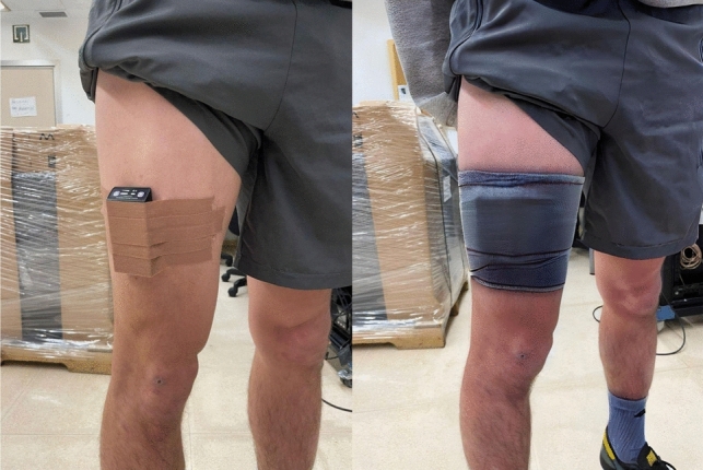 Figure 1
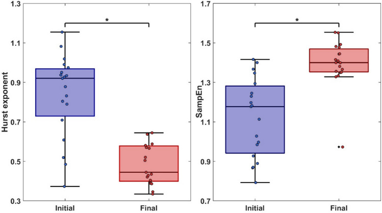 Figure 2
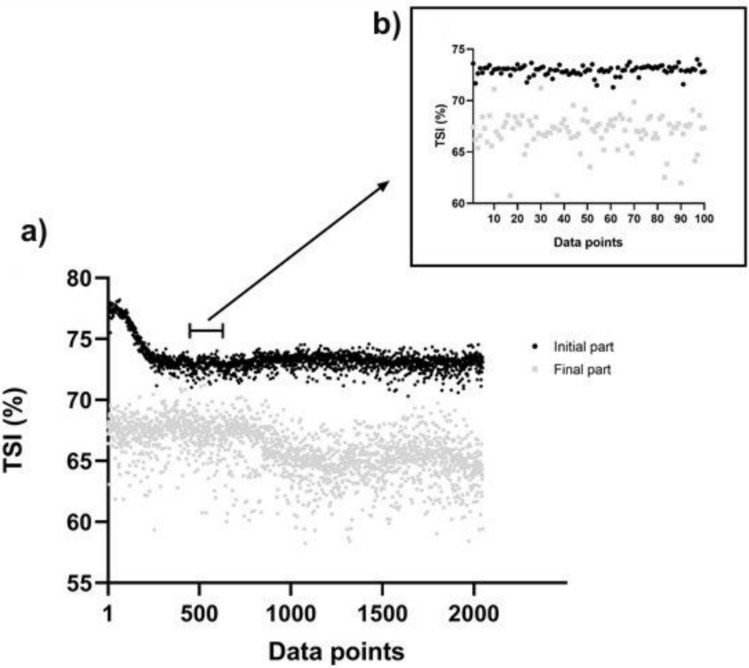 Figure 3
- —Universitat Autònoma de Barcelona
Peer Reviews
No public reviews on file for this paper yet. If you reviewed it on a platform where reviews are public (OpenReview, ICLR, NeurIPS, ICML), you can paste yours below so the community can read it here.
Videos
No videos yet. Explain this paper in a talk, walkthrough, or lecture? Add one.
Taxonomy
TopicsCardiovascular and exercise physiology · Heart Rate Variability and Autonomic Control · Non-Invasive Vital Sign Monitoring
Introduction
The time-variability structure of certain physiological and kinematic variables, such as heart rate (HR), respiratory frequency, and accelerometry, has revealed its potential in detecting changes in exercise workload and associated fatigue effects (Billat et al. 2009; Gronwald et al. 2019; Van Hooren et al. 2023; Hunter et al. 2023; Montull et al. 2025; Rogers et al. 2025). Moreover, recent studies examining electromyography and electrocardiography time series have highlighted a loss of functional connectivity in intermuscular and cardiomuscular networks with accumulated effort (Garcia-Retortillo et al. 2023; Garcia-Retortillo and Ivanov 2024). This diminished network adaptivity is often associated with uncorrelated or rigid variability of the variables under study (Balagué et al. 2020; Pethick et al. 2021; Vázquez et al. 2016, 2021).
Muscle oxygen saturation is a key indicator of the balance between oxygen delivery and consumption within the muscles, providing valuable insights into metabolic dynamics during exercise (Barstow 2019). In recent years, near-infrared spectroscopy (NIRS) has emerged as a reliable, non-invasive tool for assessing muscle oxygen saturation, gaining significant attention in sports science and medicine (Oueslati et al. 2016; Jones et al. 2016; Lucero et al. 2018; Perrey 2022). NIRS has been proven effectiveness at different exercise intensities, showing higher values of muscle oxygenation in active muscles such as vastus lateralis (Kerhervé et al. 2017; Lucero et al. 2018; Manchado-Gobatto et al. 2020; Klusiewicz et al. 2021). The applications of this tool include, for example, estimating ventilatory and lactate thresholds (Sendra-Pérez et al. 2023; Batterson et al. 2023) or comparing vascular and metabolic profiles between highly active and sedentary populations (Tuesta et al. 2024).
Tissue haemoglobin saturation index (TSI), which reflects the percentage of oxygenated haemoglobin relative to total haemoglobin (oxygenated and deoxygenated), has been commonly recorded using NIRS. A decrease in TSI may indicate an imbalance between oxygen delivery and consumption during exercise (Mairbäurl 2013; Jones et al. 2015), as well as conditions such as exposure to altitude (Martin et al. 2009; Jeffries et al. 2019), anaemia (Crispin and Forwood 2021), or peripheral vascular diseases (Bauer et al. 2004; Mesquita et al. 2013). TSI and related NIRS-derived variables have shown particular promise for assessing task disengagement and cumulative effort, with responses differing across training levels in activities such as climbing (Feldmann et al. 2020), cycling (Zorgati et al. 2015; Yogev et al. 2023), or running (Oueslati et al. 2016). Although NIRS captures responses at the microvascular level, its variables are influenced by several integrated physiological mechanisms, including cardiac pump function, blood flow, respiratory rate, muscular metabolic capacity, and even muscle activation patterns (Daniel et al. 2023; Sendra-Pérez et al. 2023; Batterson et al. 2023; Tuesta et al. 2024). As such, muscle oxygen saturation can serve as a meaningful indicator of exercise workload.
Commonly applied measures or indices for studying muscle oxygen saturation typically focus on increasing–decreasing trends, peak values, and average distributions extracted from group-pooled data (Mairbäurl 2013; Perrey et al. 2024). This methodological approach is questioned by the Network Physiology of Exercise (Balagué et al. 2020, 2022), which emphasizes the need to detect individual patterns of response to exercise and generalize from individuals to the population, rather than the other way around. In the direction of personalized physiology, the proposed methodology suggests extracting individual time series of the variables under study (instead of their peak or threshold values), detect individual variability patterns in the time series, and analyzing the nonlinear dynamics to provide deeper insights into the response to exercise (Balagué et al. 2020).
In this regard, many studies have investigated the kinetics of muscle oxygenation using first-order dynamic models, typically based on mono-exponential functions that assume stationarity and linearity, to study for example how fast a muscle becomes deoxygenated during exercise or how quickly it reoxygenated (Ferreira et al. 2005; Boone et al. 2016; Perrey et al. 2024). However, while effective in quantifying response speed and amplitude, these approaches overlook the nonlinear and time-varying nature of physiological signals, limiting their sensitivity to detect changes of fluctuations. In contrast, nonlinear methods such as Detrended Fluctuation Analysis (DFA) and Sample Entropy (SampEn) can better capture the complexity and temporal variability of oxygenation signals—offering deeper insights into physiological adaptability—yet remain poorly explored to NIRS data during exercise.
DFA is a technique used to assess self-similarity of nonstationary time series. That is, whether time series exhibit positive autocorrelation (persistent dynamics), no correlation, or negative autocorrelation (anti-persistence) (Goldberger and West 1987; Peng et al. 1994, 1995; Ihlen 2012; Eke et al. 2012). The Hurst (H) exponent, derived from DFA, has proven to be a valuable outcome for assessing the response of physiological or kinematic variables in long-term scales (Eke and Hermán 1999; Galaska et al. 2008; Vázquez et al. 2016).
The H-exponent of 0.5 represents a signal characteristic of white noise or ordinary random walk, indicating no correlation or disorder in the studied variable (Hardstone et al. 2012). H values < 0.5 reflect negative correlations or anti-persistent time series, while values > 0.5 indicate positive correlations or persistent time series (Krstacic et al. 2002; Galaska et al. 2008). For physiological variables like Heart Rate Variability (HRV), increased exercise workload often reduces H values closer to 0.5, particularly in unhealthy populations, signifying a disordered and poor physiological response (Martinis et al. 2004; Aoyagi et al. 2005). Similar trends are observed in short-term correlation metrics such as DFA-α1 (Gronwald et al. 2020; Van Hooren et al. 2023; Rogers et al. 2025). Conversely, a persistent HRV profile, commonly observed during periods of rest or low-intensity exercise, reflects a more tightly regulated response, characterized by stable variability that indicates the capacity of the system to rapidly adjust to internal or external constraints (Gronwald and Hoos 2020; Van Hooren et al. 2023; van Rassel et al. 2025; Rogers et al. 2025).
Sample entropy (SampEn) is a widely used time-variability measure that quantifies the level of regularity or randomness in time series data (Richman and Moorman 2000; Delgado-Bonal and Marshak 2019). Similar to DFA, SampEn has primarily been applied to HRV and cardiovascular variables to detect physiological disorders and evaluate exercise responses (Lewis and Short 2007; Riganello et al. 2018). Jiang et al. (2021) extended its application to oxygen saturation, reporting higher SampEn values with increased exposure to hypoxia. Higher SampEn values indicate more unpredictable dynamics or greater randomness, which can be associated with a random walk or white noise behaviour in DFA (Hardstone et al. 2012). Greater entropy in oxyhemoglobin has also been found at cortical level when increasing the intensity of a cycling endurance exercise (Hong et al. 2024). Consequently, SampEn of oxygen saturation seems potential to carry information about the physiological response under increasing stress or workload. However, the time-variability of muscle oxygen saturation and the influence of exercise intensity—from baseline to voluntary exhaustion—remain underexplored, particularly in relation to the expected shift toward less predictable and more uncorrelated dynamics at higher intensities.
This study aimed to compare the time-variability structure of the TSI, particularly through the H-exponent and SampEn, between the beginning and the end of a graded maximal exercise. Our hypothesis was that due to increase of intensity and effort accumulation at the end of the exercise: i) the H-exponent of TSI will decrease towards an uncorrelated white noise (H ≈ 0.5), and ii) SampEn of TSI will increase towards less predictable dynamics.
Materials and methods
Participants
Nineteen university students of physical education (11 females, 8 males; 21.00 ± 2.29 yrs.; 1.71 ± 0.07 m; 64.57 ± 10.06 kg), who practiced sport regularly (7.78 ± 2.20 h/week), participated voluntarily in the study. They completed a questionnaire to confirm their health status. To estimate the sample size, a large effect size (ρ = 0.82), α = 0.05, and power (1-β) = 0.95 were determined. All experimental procedures were explained to participants before they gave their written consent to participate in the study. The experiment was approved by the Local Research Ethics Committee (004-CEICGC-2024) and carried out according to the Helsinki Declaration.
Procedures
All participants, previously familiarized with the testing procedures, performed a graded maximal treadmill running test until voluntary exhaustion. The test started at 8 km/h and the velocity was increased by 1 km/h every 100 s until they could not keep the prescribed velocity. The rate of perceived exertion (RPE 6–20) scale (Borg 1998) and the HR via Polar H10 chest strap (Polar Electro Oy, Kempele, Finland) were recorded every 100 s, before changing the velocity. Consecutively prior to the running test, participants warmed up at 6 km/h for 5 min. After the test, participants walked at 6 km/h for 5 min to recover.
Data acquisition
TSI was constantly recorded, from the warm-up to the end of the test, using the PortaMon device (Artinis Medical Systems®, Einsteinweg, Netherlands), which included three light source transmitters (each one with two wavelengths between 750 and 850 nm) placed at distances of 30, 35, and 40 mm from the receiver (Jones et al. 2014; Desanlis et al. 2024). As illustrated in Fig. 1, the device was placed on the belly of the vastus lateralis of the right quadriceps, midway between the greater trochanter of the femur and lateral femoral epicondyle (Jones et al. 2014). The sampling frequency was set at 10 Hz following the recommendations by Hesford et al. (2013) and Jones et al. (2014). To secure the probe and protect it from the environmental light, a dark band was tightly wrapped around the equipment (Manchado-Gobatto et al. 2020).Fig. 1. The PortaMon device was placed and secured on the vastus lateralis of the right leg
Data analysis
We analyzed the temporal structure of the first and last 2048 raw data points of TSI time series, corresponding to 204 s each, through DFA and SampEn. Previously, the stationarity of each signal was formally assessed using the Augmented Dickey–Fuller (ADF) test. For signals where the null hypothesis of nonstationarity could not be rejected, an iterative procedure based on Empirical Mode Decomposition (EMD) was applied (Zhou et al. 2013). Specifically, the residual (global trend) was removed first, followed by successive removal of the lowest-frequency IMFs in ascending order of frequency, until the ADF test rejected the hypothesis about nonstationarity. Next the signal was normalized with mean and standard deviation of the stationary signal.
Finally, to support our findings, we performed the analysis of randomly shuffled original time series, in which correlations were destroyed but amplitude distribution preserved.
Detrended fluctuation analysis
DFA was performed as follows (according to Ihlen (2012) and Peng et al. (1995, 1994)): First, the total length of the TSI time series (N = 2048 data points) was integrated with the following equation:
\documentclass[12pt]{minimal} \usepackage{amsmath} \usepackage{wasysym} \usepackage{amsfonts} \usepackage{amssymb} \usepackage{amsbsy} \usepackage{mathrsfs} \usepackage{upgreek} \setlength{\oddsidemargin}{-69pt} \begin{document}$$Y(i)\equiv \sum_{k=1}^{i}\left[{x}_{k}- \langle x\rangle \right]$$\end{document}\documentclass[12pt]{minimal} \usepackage{amsmath} \usepackage{wasysym} \usepackage{amsfonts} \usepackage{amssymb} \usepackage{amsbsy} \usepackage{mathrsfs} \usepackage{upgreek} \setlength{\oddsidemargin}{-69pt} \begin{document}$${x}_{k:}$$\end{document} individual data point of the TSI time series.
\documentclass[12pt]{minimal} \usepackage{amsmath} \usepackage{wasysym} \usepackage{amsfonts} \usepackage{amssymb} \usepackage{amsbsy} \usepackage{mathrsfs} \usepackage{upgreek} \setlength{\oddsidemargin}{-69pt} \begin{document}$$x:$$\end{document} average TSI of the entire time series.
Then, the local trend was calculated to fit the TSI time series using a quadratic function (Ihlen 2012). Time series were divided into different windows (i.e., scales, with length n ranging from 20 to 200) (Hautala et al. 2003), in which the local trend was found. Obviously, the number of windows W depends on their length n: W_n_ = N/n. For successive n values, the magnitude of fluctuations was determined separately by substracting the local trend and constructing the final fluctuation function.
The fluctuation function was calculated in two steps. Using an integrated signal, the variance was determined in each window ν, ν = 1,…,W_n_ using the following equation (Kantelhardt et al. 2002):
\documentclass[12pt]{minimal} \usepackage{amsmath} \usepackage{wasysym} \usepackage{amsfonts} \usepackage{amssymb} \usepackage{amsbsy} \usepackage{mathrsfs} \usepackage{upgreek} \setlength{\oddsidemargin}{-69pt} \begin{document}$${F}^{2}\left(\nu ,n\right)=\frac{1}{n}{\sum }_{i=1}^{n}{\left\{Y\left[\left(\nu -1\right)\bullet n+i\right]-{y}_{\nu }(i)\right\}}^{2}$$\end{document}With.
Y(i): integrated time series.
yν(i): local trend in each window.
Finally, fluctuation function F was defined by:
\documentclass[12pt]{minimal} \usepackage{amsmath} \usepackage{wasysym} \usepackage{amsfonts} \usepackage{amssymb} \usepackage{amsbsy} \usepackage{mathrsfs} \usepackage{upgreek} \setlength{\oddsidemargin}{-69pt} \begin{document}$$F\left(n\right)=\sqrt{\frac{1}{{W}_{n}}\sum_{\nu =1}^{{W}_{n}}{F}^{2}\left(\nu ,n\right)}={n}^{H}$$\end{document}The H-exponent, derived as the slope of the linear regression between the scale n and the local fluctuations in a log–log plot, was employed to characterize the nature of TSI fluctuations for each participant during the initial and final parts of the test. Matlab^©^ R2020 was used for this analysis.
Sample entropy
SampEn measures the likelihood that time series patterns (vectors) of the m length are close to each other and will remain close in the sequence of increased length m + 1 (Richman and Moorman 2000; Delgado-Bonal and Marshak 2019). Its calculation relies on the matching consecutive points within a tolerance r in the Chebyshev distance. To ensure reliable estimation of SampEn, a systematic optimization of the input parameters m (embedding) and r was performed. We explored a specified range for both input parameters to identify the configuration best suited to our dataset characteristics and signal dynamics. SampEn was calculated across m = 2,3,4 with r changes in increments of 0.05 starting from 0.1 up to 0.5. For each (m, r) pair, SampEn was computed separately for the initial and final parts of the test. To identify optimal parameters, we applied the following criteria that must be present in both phases: i) low inter-individual variability, defined as a coefficient of variation (CV = SD/mean) below 0.1; ii) robustness to changes in r, indicated by the a plateau-like SampEn values across increasing r, for a given m; iii) computational complexity – when multiple configurations satisfied the above conditions, a pair with the lowest m and r was selected. In result, m = 2 and r = 0.35 was found as optimal for TSI time series.
SampEn is defined by a negative logarithm, in which the average number of sequences under the tolerance is considered for both lengths m + 1 (in the numerator) and m (in the denominator). Low entropy values arise from regular physiological time series (like those with rhythmic fluctuations, Kosciessa et al. (2020)), and higher values reflect more random, irregular behaviour (Costa et al. 2005). Also, high values are typical for stochastic data sets (Lake and Moorman 2011; Weippert et al. 2014). Matlab^©^ R2020 was used for this analysis.
Statistics
Wilcoxon matched pairs test was used to compare average values, H-exponents and SampEn of TSI between the initial and final parts of the exercise. The significance level for the statistical tests was set at p = 0.05. Cohen’s d was estimated for the test statistics Z of the previous analysis to demonstrate the magnitude of standardized mean differences (Fritz et al. 2012). According to Cohen's (1988) guidelines, d ≥ 0.2, d ≥ 0.5, and d ≥ 0.8 represent small, intermediate, and large effect sizes, respectively. Statistical analyses were performed with SPSS v.15 (SPSS Inc., Chicago, USA).
Results
The maximum velocity of the test was 15.74 ± 1.85 km/h, while the maximum HR was = 191.63 ± 6.55 bpm, and the maximum RPE was 19.01 ± 0.81. The mean values of HR and RPE from the initial and final 204 s, corresponding to the analyzed sections, was HR = 134.72 ± 9.83 bpm and RPE = 8.94 ± 1.17 at the beginning, and HR = 186.37 ± 6.28 bpm and RPE = 18.79 ± 0.73 at the end, respectively.
TSI average values largely decreased from the initial (68.24 ± 2.53%) to the final part (61.03 ± 2.50%) of the graded maximal running test (Z = -3.58, p < 0.01; d = -2.88).
The comparison of the time-variability of TSI between the initial and the the final part was as follows (see Fig. 2):
- H-exponents largely decreased from H = 0.84 ± 0.21 at the beginning to H = 0.49 ± 0.10 at the end of the exercise (Z = -6.84, p < 0.01; d = -1.57).
- SampEn largely increased from 1.12 ± 0.20 at the beginning to 1.40 ± 0.13 at the end of the exercise (Z = -5.11, p < 0.01; d = 1.17). Fig. 2. Box-plots illustrating the decrease of Hurst exponent (left) and increase of Sample entropy (SampEn) (right) of the Tissue saturation index (TSI) between the initial and final parts of the running test.
As illustrated in Fig. 3, with an example of one participant, the time-variability of TSI at the final part is larger compared to the initial. The fluctuations in the final part tended to be uncorrelated and random, resembling white noise. In contrast, the initial part exhibited more moderate persistence, characterized by a smoother pattern of tight increases and decreases.Fig. 3. Example of raw Tissue saturation index (TSI) fluctuations at the initial (black, upper values) and final (grey, lower values) parts of the graded maximal exercise from one participant (a: the analyzed 2048 data points; b: zoom of 100 data points)
At the end of the analysis, we introduced data shuffling after preprocessing to validate our findings. This randomization preserved the amplitude distribution of the signal while fully disrupting temporal correlations. As expected for uncorrelated white noise, the H-exponent in the shuffled data was consistent across both parts: 0.49 ± 0.03 (initial) and 0.49 ± 0.03 (final). In contrast, the original detrended signals from the initial part exhibited a substantially higher mean Hurst exponent of 0.84 ± 0.21, confirming the presence of long-range correlations.SampEn values were generally higher in the shuffled data, reflecting their greater unpredictability. In the final part, entropy changed only slightly after shuffling—from 1.40 to 1.57—suggesting that this part was already highly irregular following preprocessing.
Discussion
This study, which aimed to investigate the effects of exercise intensity on the time-variability of muscle oxygen saturation, found that by the end of a graded maximal running exercise, the TSI fluctuations changed toward uncorrelated or disordered patterns, resembling random white noise. In contrast, at the beginning of the exercise, the TSI fluctuations were persistent and less variable, which can be related to a more tightly regulated response (Krstacic et al. 2002; Aoyagi et al. 2005; Gronwald et al. 2020; Van Hooren et al. 2023). These findings provided evidence that the time-variability structure of TSI was sensitive to the effects of the accumulated effort and increasing intensity during a graded running exercise.
Consistent with previous studies, the decrease in TSI observed at the end of the test likely reflects an imbalance between oxygen consumption and delivery. This reduction may be attributed to factors such as lowered pH, elevated lactate levels, lowered Hb-O_2_ affinity, increased temperature, or hemodynamic redistribution during high-intensity exercise (Mairbäurl 2013; Jones et al. 2015; Boezeman et al. 2016). Assessed indicators such as elevated HR and RPE, both associated with acute fatigue effects, further supported the presence of high-intensity effort. These results suggested that both the quantitative values of TSI and the qualitative changes in its fluctuations may complementary reflect aspects of metabolic strain and effort accumulation.
The observed tendency of the H-exponent approaching 0.5 and the increase in SampEn of TSI at the end of exercise align with physiological findings from previous studies on HRV, inter-breath intervals, and other cardiorespiratory variables in response to exercise effort (Krstacic et al. 2002; Garcia-Retortillo et al. 2017; Gronwald et al. 2019; Rogers et al. 2025) or to other stressors such as hypoxia and disease conditions (Scafetta et al. 2007). These results may reflect a reduction in the functional connectivity of regulatory mechanisms governing muscle oxygen concentration, likely involving inter-muscular, cardio-muscular, or cardio-respiratory networks (Balagué et al. 2016; Garcia-Retortillo et al. 2023; Garcia-Retortillo and Ivanov 2024).
Future research should offer a comprehensive network analysis of the time-variability structure of multilevel physiological variables, including muscle oxygen saturation, to elucidate their synergistic interrelations, potential time delays, and how these insights could collectively inform about the system's response to increasing workloads (Ivanov and Bartsch 2014; Balagué et al. 2020; Ivanov 2021). As there is a lack of available technology informing about the muscle metabolism dynamics during exercise, muscle oxygen saturation can contribute notably to the study of vertical network synergies across different organismic levels, such as tissues and organs (e.g., TSI and heart rate), occurring during exercise. Until now, only the dynamics of meso- and macroscopic variables such as muscle electrical activity, heart electrical activity, or accelerometry, integrating a broader range of physiological processes (e.g., metabolic, contractile, reflexive, volitional, among others), could help to provide an integrated assessment during exercise (Haken 1983; Balagué et al. 2020; Vázquez et al. 2021).
The temporal variability of muscle oxygen saturation may be particularly useful for detecting exercise intensity and related-fatigue effects during endurance activities, as it reflects underlying cardiorespiratory and metabolic demands (Mairbäurl 2013; Oueslati et al. 2016). While HRV has been widely applied to detect exercise workload in endurance activities (Gronwald et al. 2019; Mateo-March et al. 2023; Van Hooren et al. 2023; Rogers et al. 2025), its usefulness in resistance exercises remains less clear (Weippert et al. 2013; Kingsley and Figueroa 2016; Cauwenberghs et al. 2021). Thus, further research should evaluate the applicability of muscle oxygen saturation variability across different types of exercises. In addition, incorporating the intermediate phase of exhausting exercises—characterized by increased fluctuations as a transitional phase between stable and unstable states—may offer an alternative and potentially insightful approach for identifying critical points related to physiological thresholds in individual-specific contexts.
The sensitivity of muscle oxygen saturation time-variability to exercise intensity highlights its potential for developing monitoring tools to assess athlete’s health and performance. These tools could benefit from analyzing intra-individual variability of nonstationary time series rather than relying solely on tendencies, discrete values, or average distributions (Balagué et al. 2020). Time series analysis might offer a promising approach for detecting nonlinear events associated with exercise, including not only effort accumulation but also training effects (Garcia-Retortillo et al. 2017), task failure (Vázquez et al. 2016), overtraining (Tian et al. 2013; Armstrong et al. 2022), or injury risk (Pol et al. 2019; Fonseca et al. 2020). Early warning signals—reflected in alterations to the temporal structure of fluctuations, such as rising uncorrelated patterns—can reveal diminishing system adaptability and help anticipate critical transitions before adverse events occur (Scheffer et al. 2009). To fully realize this monitoring potential to practice, technological improvements are necessary in NIRS systems to ensure reliable signal acquisition and real-time variability analysis.
Future studies should address methodological limitations of this study and challenges on the reliability of NIRS, such as minimizing external noise effects (e.g., light interference or gait impact on muscle oxygen saturation), enhance light sources to increase tissue penetration, accounting for the influence of ventilatory work at high workloads (Thiel et al. 2011; Oueslati et al. 2016; Jeffries et al. 2019), as well as the effects of high skinfold thickness by particularly assessing the fat layers of individuals (Stuer et al. 2024). Additional NIRS-derived variables, such as oxyhemoglobin and deoxyhemoglobin, and relevant muscles during running such as gastrocnemius may also be included in analyses (Hiroyuki et al. 2002). Researchers are warranted to examine how time-variability in muscle oxygen saturation is affected by factors such as time series length, sampling frequency, exercise protocols and performance levels (Eke et al. 2012; Gronwald et al. 2020; Tuesta et al. 2024). Finally, advanced analytical methods, including Bayesian approaches for improving H-exponent estimation (Likens et al. 2023) and multifractal analyses (Kokosińska et al. 2018; Racz et al. 2018), should be considered to enhance the reliability and depth of time-variability assessments.
Conclusions
The time-variability of muscle oxygen saturation shows promise as a sensitive indicator of exercise intensity during graded maximal running. The measure could serve as a valuable tool for the early detection of exhaustion and exercise tolerance, providing critical insights into individual responses to varying workloads. Further investigation is required to establish the time-variability of muscle oxygen saturation as a reliable and non-invasive measure for assessing exercise load and performance. Additionally, future research should explore muscle oxygen saturation to advance in the study of vertical network synergies during exercise.
Conflict of interest
The authors declare no conflict of interest. This research did not receive any specific grant from funding agencies in the public, commercial, or not-for-profit sectors.
The reference list from the paper itself. Each links out to its DOI / PubMed record.
- 1Likens AD, Mangalam M, Wong AY, et al (2023) Better than DFA? A Bayesian Method for Estimating the Hurst Exponent in Behavioral Sciences. Ar Xiv ar Xiv:2301.11262 v 1