Recent advancements in integer-valued autoregressive models for count data time series: A comprehensive review
Vinitha Serrao, Satyanarayana Poojari, Asha Kamath

TL;DR
This paper reviews recent developments in modeling time series with count data, focusing on improved methods for handling complex statistical features.
Contribution
The paper provides a comprehensive review of recent advancements in integer-valued autoregressive models and identifies future research directions.
Findings
Recent research has focused on novel thinning operators and flexible innovation distributions for count data.
The review highlights trends and methodological gaps in modeling count time series.
Unified frameworks are being developed to handle multiple data characteristics simultaneously.
Abstract
Count data time series, characterized by non-negative integer values, frequently arise across diverse domains, including finance, public health, economics, epidemiology, and environmental sciences. Such series often exhibit characteristics such as equidispersion, overdispersion, underdispersion, and zero-inflation/deflation. Failure to appropriately account for these features can result in biased parameter estimates and misleading statistical inference. This review presents a comprehensive overview of recent methodological developments in integer-valued autoregressive (INAR) models, with particular emphasis on thinning operators, estimation methods, and model extensions. A systematic literature search was conducted using electronic databases, including Scopus and Google Scholar, to identify relevant studies published between 2010 and 2024. Recent research has primarily focused on the…
Click any figure to enlarge with its caption.
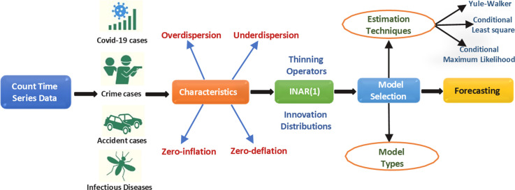 Figure 1
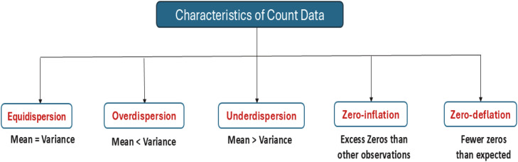 Figure 2
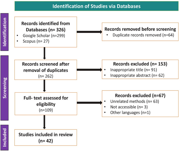 Figure 3
Peer Reviews
No public reviews on file for this paper yet. If you reviewed it on a platform where reviews are public (OpenReview, ICLR, NeurIPS, ICML), you can paste yours below so the community can read it here.
Videos
No videos yet. Explain this paper in a talk, walkthrough, or lecture? Add one.
Taxonomy
TopicsCOVID-19 epidemiological studies · Statistical Methods and Bayesian Inference · Financial Risk and Volatility Modeling
Specifications table.Subject areaMathematics and StatisticsMore specific subject areaTime Series AnalysisName of the reviewed methodologyModels addressing various dispersion patterns, zero-inflation, and zero- deflation in count data time series.KeywordsCount data time series, Underdispersion, Overdispersion, Zero-inflation, INAR (1) model.Resource availabilityNot Applicable.Review question
- •What are the existing modeling approaches for handling various dispersion patterns in count time series data, and how do these models differ in terms of structure, innovation distributions, thinning mechanisms, and estimation methods?
- •What are the existing modeling approaches for handling zero-inflation and deflation patterns in count time series data, and how do these models differ in terms of structure, innovation distributions, thinning mechanisms, and estimation methods?
- •What are the key developments in thinning operators used in INAR (1) models?
Background
Count data time series, consisting of discrete events recorded at regular intervals, are prevalent across many scientific fields, including road accidents [1], economic indicators [2], COVID-19 deaths [3], influenza cases [4], and criminal incidents [5].These applications are closely linked to several SDGs, including SDG 1 (No Poverty), SDG 2 (Zero Hunger), SDG 3 (Good Health and Well-Being), SDG 8 (Decent Work and Economic Growth), SDG 11 (Sustainable Cities and Communities), and SDG 16 (Peace, Justice, and Strong Institutions). For example, analyzing road accidents can inform strategies to improve urban safety and transportation planning, monitoring disease cases can support public health initiatives, studying crime patterns can strengthen justice systems and examining economic indicators can identify vulnerable populations and guide poverty alleviation programs. By providing insights into these critical areas, INAR models can help guide evidence-based policies that contribute to achieving the SDGs.
One of the main challenges in modeling and forecasting count time series is addressing unique features such as equidispersion, overdispersion, underdispersion, zero-inflation, and zero-deflation, as clearly illustrated in Fig. 1. If these features are not properly addressed, the resulting forecasts may be inaccurate, potentially leading to misleading conclusions [6].Fig. 1. Characteristics of count data.Fig. 1: dummy alt text
For large count datasets, continuous time series models like ARIMA can be applied, leveraging the central limit theorem, which states that discrete distributions (e.g., Poisson, Binomial, Negative Binomial) converge to a normal distribution under certain conditions [7]. However, ARIMA models are often unsuitable for count data and discrete-valued series because they assume real numbers and normally distributed errors. As a result, specialized models for count data have been proposed, although they still face limitations in addressing overdispersion effectively.
To address these limitations, INAR models introduced by McKenzie [8] and Al-Osh and Alzaid [9] have gained prominence. These models extend classical autoregressive models by incorporating integer-valued distributions, which enable them to handle serial correlation and capture the distributional properties of discrete data more effectively. The INAR (1) model is represented as:
where is the observation at the time t and the operator is referred to as the binomial thinning operator, given by [10]. This operator indicates that there is a probability of a previous count being carried over to the current period. This relationship can also be expressed as where represents a binomial distribution with trials and success of probability Additionally, represents a sequence of uncorrelated, non-negative, integer-valued random variables characterized by a mean of and a variance of
To illustrate parameter estimation in the INAR (1) framework, consider a public health application in which denotes the daily number of influenza cases in a region. One commonly used estimation approach is CLS, based on the conditional expectation
The CLS estimators of and are obtained by minimizing the sum of squared deviations between the observed counts and their conditional expectations. For instance, an estimated thinning parameter implies that, under the binomial thinning operator, approximately 65% of the cases from the previous time point are expected to persist into the current period. The estimated innovation mean reflects the average number of new cases arising independently of past observations.
YW estimation provides an alternative moment-based approach, exploiting the theoretical relationships between the mean, variance, and autocovariance of the INAR (1) process. Due to its computational simplicity, the YW method is particularly suitable for large datasets. When the distribution of the innovation process is specified, CML estimation can also be employed and generally yields more efficient parameter estimates.Although the INAR (1) model is considered efficient, it still faces challenges, particularly in addressing overdispersion, underdispersion, and zero-inflation, which are common in real-world count time series data. Traditional count data models often struggle with these complexities, resulting in inadequate model fit and poor predictive performance. This review explores advancements in INAR (1) models from 2010 to 2024, specifically those designed to address equidispersion, overdispersion, underdispersion, and zero-inflation/deflation in count time series. By examining a broad set of characteristics within a single framework, the review helps researchers identify suitable models and estimation techniques aligned with specific data characteristics, thereby improving estimation and forecasting accuracy. This comprehensive review offers a clear understanding of the strengths and limitations of existing models and provides a foundation for identifying research gaps and guiding future developments in count time series modeling.
Method details
Search strategy
The articles reviewed in this manuscript were obtained from the Google Scholar web search engine and the Scopus database, covering the period from 2010 to December 2024.The search utilized keywords such as
- i."count data time series" AND "overdispersion"
- ii."time series of count" AND "zero-inflation" OR "zero-deflation"
- iii."count data time series" AND "overdispersion" AND "underdispersion".
Before the screening process, duplicate articles were removed to ensure a unique set of sources. The review focused on peer-reviewed journal articles, review papers, conference proceedings, and other key contributions published in the English language. This process resulted in a total of 326 articles, including 299 articles from Google Scholar and 27 articles from Scopus.
The screening process was conducted in stages, beginning with an evaluation of the article titles, followed by the abstracts, and finally the methods sections. This process resulted in a final set of 42 articles selected for detailed review. The specific inclusion and exclusion criteria are outlined below.
Inclusion criteria
- •The title and abstract include relevant keywords
- •The article is written in the English language
- •The article is published in a journal or conference proceedings
- •The study includes the development of relevant methods
Exclusion criteria
- •Duplicate articles
- •Articles written in languages other than English
- •Articles addressing unrelated methods
- •Articles that are not accessible
A total of 326 articles were initially retrieved, and after applying the inclusion and exclusion criteria, 42 articles were selected for this review. The procedure followed during the article selection process is presented in Fig. 2.Fig. 2PRISMA flow chart.Fig. 2: dummy alt text
Question-1: What are the existing modeling approaches for handling various dispersion patterns in count time series data, and how do these models differ in terms of structure, innovation distributions, thinning mechanisms, and estimation methods?
Models addressing various dispersion patterns
This section is organized into four categories: (1) models specifically suited for handling overdispersion; (2) models designed to address underdispersion; (3) models capable of managing both overdispersion and underdispersion; and (4) models that simultaneously account for equidispersion, overdispersion, and underdispersion. This structured approach provides researchers with a clear framework to select the most appropriate models and estimation methods based on the distinct characteristics of the count data time series they are analysing. By categorizing models in this manner, it enhances the ability to choose suitable techniques for more accurate analysis and forecasting.
Models handling overdispersion
Overdispersion is a common issue in medical studies, often resulting from positive correlations between monitored events [11]. To handle overdispersion, various statistical models have been developed. The Negative Binomial distribution is commonly employed for modeling count data that exhibits overdispersion followed by quasi-poisson, and zero-inflated models ( [[12], [13], [14]]). However, these models sometimes underestimate standard errors and overstate the significance of certain covariates. To address the challenges of modelling overdispersed count time series, INAR models have become increasingly popular. To account for overdispersion, two main approaches have been proposed:
- a.modifying INAR (1) models by using alternative marginal distributions and thinning operators
- b.adapting the binomial thinning operator to handle different innovation distributions.
Various INAR (1) models address overdispersion in count time series. Initially, [15] proposed the NG-INAR (1) model, which uses a Negative Binomial thinning operator ( ) to extend the PINAR (1) model. Key estimation methods include MLE, YW, and CLS. The INAR (1) model with Geometric innovations proposed by [16] adopts CML and AFML methods for parameter estimation. By introducing a generalized binomial thinning operator ( ), [17] formulated the first-order dependent counting geometric INAR model. The study employed CLS and MLE methods for parameter estimation. As a further advancement, [18] introduced a CP-INAR (1) model with a binomial thinning operator ( ). A test for overdispersion in INAR models was developed by using the property that a CP-INAR (1) model exhibits strong mixing properties characterized by weights that decrease exponentially. The INAR (1) model with a Poisson-Geometric marginal distribution, presented by [19] utilizes a two-step CLS estimation procedure to extend the functionalities of the PINAR (1) and GINAR (1) models. Building on this, [20] introduced a stationary INAR (1) model with Poisson-Lindley innovations, employing CLS, YW, and MLE for estimation. To accommodate heavy tailed count time series, [21] introduced an INAR (1) model incorporating Generalized Poisson inverse Gaussian innovations into the INAR(1) framework. This model accommodates both equidispersion and overdispersion and is also well-suited for count data with a high frequency of zero values with CML method for parameter estimation. Recently, [22] evaluated the performance of the ACP and PAR models, concluding that the ACP model is preferable across different sample sizes.
Models handling underdispersion
Underdispersion can occur due to model overfitting or small sample sizes [23]. Several widely recognized parametric models are available for analyzing underdispersed count data. These include the Generalized Poisson distribution introduced by [24], the Double Poisson distribution proposed by [25], and the Conway-Maxwell Poisson distribution developed by [26]. Each of these models is characterized by two parameters. However, these models have limitations in effectively describing underdispersion. To address this issue, [27] explored the performance of a stationary INAR (1) process with two-parameter Good and Power Law distribution innovations, which demonstrated better properties for modeling underdispersed counts. However, extending these models to higher-order autoregressive structures, such as INAR(p) developed by [28], introduces further complexity. Notably, even if the innovations are underdispersed, the resulting INAR(p) process does not necessarily retain this property in the observed data. This limitation highlights an important direction for future research. Although underdispersion has received little attention in practical data analysis, it highlights the need for specialized models to effectively address this phenomenon.
Models handling both overdispersion and underdispersion
Several models have been developed to address overdispersion and underdispersion simultaneously in count data, [29] introduced an INAR (1) model with power series innovations, using YW, CLS, and MLE for estimation. To address underdispersion within a hidden Markov framework, the Poisson- hidden Markov model was modified by [30] by replacing the Poisson distribution with the CMP distribution, resulting in the CMP-HMM model. A novel thinning operator based on the GSC distribution (⋄) was introduced by [31], leading to the development of an INAR (1) model estimated using CLS, weighted CLS, and MQL methods. In a related study, [32] introduced an extended binomial thinning operator (⊚), which featured two parameters, offering greater flexibility in modeling. Their work presented the EBINAR (1) model and explored two-step CLS estimation for the innovation-free case, alongside a discussion of CML estimation method. Later, [33] developed a flexible INGARCH model using the generalized CMP distribution which introduces an additional parameter to manage heavy tail behaviour, with parameters estimated using the CML method. Recently, [34] introduced an ZDGG-INAR (1) model. This model addresses the limitations of the GPIG-INAR (1) model and effectively captures all the characteristics such as zero-inflation/deflation, zero truncation, along with dispersion. The parameters of the ZDGG-INAR (1) model were estimated using methods such as YW, CLS, CML, and Bayesian approaches, making it a versatile tool for handling various count data characteristics within the INAR framework. This is the only model found in the literature that is suitable for all the characteristics of count data, and it is based on the INAR (1) framework.
Models handling equidispersion, underdispersion and overdispersion
Models that address all three types of dispersion offer considerable flexibility and wide applicability in analysing various types of count data. The adaptability of the CMP model was emphasized by [35] using MLE for estimation. This model can also effectively manage both zero-inflation and zero-deflation in count data. Later, [36] developed an INAR (1) framework that integrates Bernoulli-Geometric marginal distributions and utilizes a generalized thinning operator ( ), providing enhanced flexibility for count data modeling, with parameters estimated via MLE. Similarly, [37] proposed an INAR (1) model using Katz family innovations, which incorporates Poisson, Negative Binomial, and binomial distributions to capture a variety of dispersion patterns. Although both CML and MLE methods can be applied, the practical implementation of these models is challenging due to the complexity of the marginal distribution, which often lacks a closed-form expression.
Motivated by the ability of the Double Poisson and Generalized Poisson distributions to capture various dispersion patterns and their relatively simple probability mass functions, [38] expanded the INAR (1) process by developing the DP-INAR (1) and GP-INAR (1) models. This model uses Poisson innovations and binomial thinning ( ) to capture different dispersion patterns. Model parameters are estimated using methods such as CML, CLS, and YW, and a test is developed to identify the types of dispersion. A related extension incorporating a generalized Poisson thinning operator (⊛) was explored by [39]. Model parameters were estimated using CLS, MQL and CML methods. Additionally, [40] proposed a shifted INAR (1) model with Borel innovations. This model utilized binomial thinning ( ), with parameters estimated via YW, CLS, and CML methods and constructed a test for dispersion. More Recently the WNBL distribution based INAR(1) process presented by [5] combines binomial thinning operator ( ) with WNBL innovation, where the innovation distribution is constructed as a weighted combination of the traditional negative binomial and size-based negative binomial distributions, offering flexibility through adjustable parameters. Model parameters were estimated using CML, YW, and CLS methods and applied to real-world datasets from criminology and epidemiology, demonstrating its practical relevance and versatility.
Question-2: What are the existing modeling approaches for handling zero-inflation and deflation patterns in count time series data, and how do these models differ in terms of structure, innovation distributions, thinning mechanisms, and estimation methods?
Models handling zero-inflation and zero-deflation
Count data frequently show an excess of zeros, known as zero-inflation, a concept formally introduced by [41] and [42]. Zero-inflated models, which combine a degenerate distribution at mass zero with a count distribution such as Poisson or Negative Binomial, were developed to address this issue. To address the problem of zero-inflation, [43] made significant advancements with the introduction of a generalized linear model using the ZIP distribution, which was specifically designed for a manufacturing process where additional zeros resulted from transitions between flawless and defective production states. Further, [44] expanded on this concept to include zero-deflation, thereby creating the zero-modified Poisson regression model.
The ZIP model is appropriate for datasets displaying equidispersion. However, for datasets with a high prevalence of zero counts, other distributions like the ZINB distribution [45] and the zero-inflated CMP distribution [46] have been developed as alternatives. The ZINB model addresses both excess zeros and overdispersion by considering population heterogeneity, where the probability of zero counts varies among individuals. Unlike the ZIP model, which is designed primarily for equidispersed data, the ZINB model is more suitable for datasets with both excess zeros and overdispersion [43].
Recent advancements include the development of various INAR processes to model zero-inflated and zero-deflated count time series. The- ZIP-INAR (1) model introduced by [47] merges the INAR (1) process with ZIP innovations to manage excess zeros using CML and AFML estimation methods. Related extensions within the INGARCH models were presented by [48], where ZIP and negative binomial INGARCH models were proposed and fitted to real-world datasets using the EM algorithm.
Within the state-space framework, [49] introduced a flexible state-space model that uses the ZINB distribution. Due to the limitations of traditional estimation techniques like the Kalman filter and Kalman smoother, the study utilized a Monte Carlo-based Expectation-Maximization algorithm, which includes particle filtering and smoothing for parameter estimation. The study also developed an R package ZIM (Zero Inflated Models) to support the application of this model. A new ZIP-INAR (1) model was considered by [50], where the PINAR (1) process was combined with an independent Bernoulli process utilizing YW, CLS, and MLE estimation methods. To address the shortcomings of the ZIP-INAR (1) model, [51] ZMG-INAR (1) model and introduced a test for detecting zero-inflation/deflation based on the model.
The innovation structure of the ZMG-INAR (1) model introduced by [51] is complex due to its intricate innovation structure and restrictive parameter conditions. To address this, [52] proposed an INAR (1) process with ZMG innovations, employing binomial thinning ( ). This model also accommodates equidispersion, underdispersion, and overdispersion, and its flexibility is enhanced by encompassing the GINAR (1) model as a special case. The parameter estimation used were CML, YW, and CLS. Additionally, flexibility in handling diverse zero patterns was achieved by [53] through the extension of the binomial autoregressive model - introducing four variants: (i) BAR (1) Process with zeros at random; (ii) BAR (1) Process with innovational zeros; (iii) Zero inflated binomial thinning for AR (1) model; (iv) BAR (1) Process with zero threshold. These models address various zero structures in count data using maximum likelihood estimation. Additionally, [54] proposed the generalized zero-modified geometric distribution along with a new thinning operator based on zero-modified geometric counting series, using maximum likelihood estimation. Finally, an INAR based model incorporating a randomized binomial thinning operator ( ) and a zero-inflated geometric distribution featuring random coefficients was examined by [55]. The model employs CLS and MLE techniques, providing greater adaptability for analyzing count time series with complex patterns.
Count data with an abundance of zeros and ones, common in sectors like insurance and industry, is relevant to SDGs 1 (No poverty), 8 (Decent work and economic growth), 9 (Industry, innovation and infrastructure), and 12 (Responsible consumption and production). Traditional INAR (1) models, including Geometric and Poisson variants, often struggle to accurately capture these data patterns. For instance, GINAR (1) models tend to overestimate zero counts and underestimate one counts, whereas PINAR (1) models exhibit the opposite behaviour. Additionally, existing zero-inflated and CP-INAR (1) models face similar limitations. To address these challenges, [7] introduced a novel mixture of GINAR (1) processes designed for overdispersed count time series with high proportions of zeros and ones. The estimation methods used were YW and QMLE. To further accommodate the higher prevalence of zeros and ones in count data, the zero-and-one inflated Poisson distribution was also introduced with the foundational contributions provided by [56] along with [57].Building on this, [58] proposed the ZOIP-INAR (1) model, which combines the ZOIP distribution with the INAR (1) process. This model effectively captures count time series with excess zeros and ones, as well as overdispersion or underdispersion.
A copula-based time series regression model incorporating covariates was introduced by [59] to effectively manage zero-inflation. Flexibility in modelling dependent count time series was enhanced by [60] through the development of a generalized Negative Binomial thinning operator ( ) with the parameter estimation conducted using YW, CML, and modified CLS methods. Expanding on the modelling of zero-inflated count data, [61] constructed an INAR (1) process with zero-modified Poisson-Lindley innovations, employing binomial thinning for zero-modified count time series, with estimation methods including YW, CML, and CLS. Building on this, [4] proposed a more comprehensive framework using zero-modified Power Series distributions within a Generalized Autoregressive Moving Average model. This approach provides flexibility, with parameter estimation performed using Bayesian methods via a Hamiltonian Monte Carlo simulation algorithm.
Additionally, [62] introduced a first-ordered integer-valued moving average process using Zero-modified Geometric innovations based on a binomial thinning operator ( ) for analysing count data with short-run autocorrelation. This model also effectively captures data exhibiting equidispersion, overdispersion, and underdispersion. Parameter estimation was performed using CML estimation method. A novel approach for modeling zero-modified count time series was introduced by [63] through the zero-modified stochastic conditional duration models,where latent Markov sequences generate intensities for zero-modified Poisson and zero-modified negative binomial distributions within a generalized state space framework for modeling count data with excess or deficit of zeros. Parameter estimation is facilitated through a generalized state-space form. Addressing the limitations of conventional INAR (1) models in modeling periodic count data, [64] introduced PZIP-INAR (1) model. This model specifically targets overdispersion caused by excessive zeros in time series with periodic patterns. By incorporating periodically varying zero probabilities within a Poisson process framework, the PZIP-INAR (1) model offers a more suitable approach for analysing such data, utilizing CML, YW, and CLS estimation methods. Finally, dependence in the thinning mechanism was proposed by [65] through- Neyman type A thinning operator ( ), resulting in a stationary INAR (1) process with a Geometric INAR (1) innovation structure, where parameters were estimated using CMLE, modified CLS, and YW approaches.
Recent advancements in integer-valued autoregressive models have improved the flexibility and accuracy of count data time series analysis, addressing equidispersion, overdispersion, underdispersion, and zero-inflation. The most commonly used estimation methods are CML, YW, and CLS. As complex count datasets continue to emerge, further development in model structure and estimation techniques will be crucial for capturing unique data characteristics and enhancing decision-making across various fields.
Question-3: What are the key developments in thinning operators used in INAR (1) models?
Thinning operators
A widely used class of models for count time series is the INAR (1) family, which utilizes thinning operators. A thinning operator is a probabilistic tool that reduces a random count variable to a smaller integer-valued variable. This mechanism is especially effective for defining in terms of ensuring that retains its integer nature.
Table 1 provides an overview of various thinning operators, along with their associated mathematical formulations and corresponding practical examples, highlighting application scenarios in which these operators can be effectively employed. This facilitates a clearer understanding of their practical relevance. The table also illustrates the progression from binomial thinning to the GNTA thinning operator through the incorporation of increasingly flexible random variable distributions.Table 1. Overview of thinning operators and their mathematical operations.Table 1: dummy alt textName along with proposed authorOperatorOperation****-Practical ExampleBinomial thinning operatorSteutel and van Harn (1979) [10] is the i.i.d Bernoulli random variables
- •Daily count of visits to the web site of the “statistical calendar”.
- •Counts of utilization of the examination room of the emergency department of a children’s hospital.
- •Monthly counts of robbery. Signed Binomial thinning operatorKim and Park (2008)[66] is the i.i.d. Bernoulli random variables.
- •Monthly numbers of new patients diagnosed with AIDS Signed generalized power series thinning operatorZhang et al. (2010)[67] is the i.i.d. generalized power series distribution.
- •Count of drugs reported in the police car beat Negative Binomial thinning operatorRistic et al., (2009)[15]* is the i.i.d Geometric random variables
- •Count of sex offences Generalized Binomial thinning operatorRistic et al., (2013)[17]°θ Here where is the sequence of i.i.d. random variables with Bernoulli distribution, is the sequence of i.i.d. random variables with Bernoulli distribution and is a random variable with Bernoulli distribution.
- •Monthly counts of vagrancy offences Generalized Poisson thinning operatorKai Yang et al., (2019)[39] Here max is the i.i.d Generalized Poisson random variables
- •Monthly claims count.
- •Monthly family violence counts. GSC thinning operatorKang et al. (2020)[31] where is the sequence of i.i.d.
- •Monthly count of criminal mischief.
- •Number of different IP addresses. Generalized Negative Binomial thinning operatorShamma et al. (2020)[60] Here where be a sequence of i.i.d. random variables with geometric distribution and is a Bernoulli random variable
- •Weekly counts of Hantavirus disease. Extended Binomial thinning operatorLiu and Zhu (2021)[32] [ where { be a sequence of i.i.d. random variables with common distribution
- •Monthly tallies of crime data.
- •Stock data in New York Stock Exchange.
- •Crimes of family violence GNTA thinning operatorAmiri et al. (2024)[65] where is the dependent zero-inflated Bell distribution (ZIBe) random variable with parameters
- •Monthly counts of drug calls.
- •Daily counts of COVID-19.
- •Weekly counts of Tularemia disease
The Table 2 summarizes studies from 2010 to 2024, highlighting the models used, estimation methods applied, performance measures evaluated for both simulation and empirical study, and the characteristics of count data addressed.Table 2. Summary of INAR (1) models, estimation methods, performance measures and characteristics (2010–2024).Table 2: dummy alt textAuthorsModels usedEstimation MethodsPerformance MeasuresCharacteristics of count dataMansour Aghababaei Jazi, Geoff Jones, Chin-Diew Lai(2012) [16]GINAR (1), INAR (1)CML, AFMLMSE, AICOverdispersionMansour Aghababaei Jazi, Geoff Jones, Chin-Diew Lai(2012) [47]INAR (1), ZIP-INAR (1)CML, AFMLMSE, AICZero-inflationFukang Zhu (2012) [48]Poisson INARCH (2), ZIP-INGARCH (2),NB1-INARCH (2), NB2-INARCH (2),ZINB1-INARCH (2), ZINB2-INARCH (2)Expectation Maximization algorithmMADE, AIC, BICZero-inflation, overdispersionChristian H. Weiß (2013) [27]PINAR (1), GP-INAR (1), GP-INARCH,Good INAR (1), Power Law INAR (1)MLEAIC, BICUnderdispersionSebastian Schweer, Christian H. Weiß (2014) [18]Poi-INAR (1), INARCH (1),NB-INAR (1), Poi_2_-INAR (1), Poi_3_-INAR (1)CMLAIC, BICOverdispersionMing Yang, Joseph E Cavanaugh, Gideon KD Zamba(2015) [49]Dynamic models: Poisson + AR (1),NB + AR (1), ZIP + AR (1), ZINB + AR (1)Monte-Carlo Expectation Maximization algorithmAICOverdispersion,Zero-inflationMiroslav M. Ristić, Aleksandar S. Nastić and Ana V. Miletić Ilić(2013) [17]PINAR (1), NG-INAR (1), Mixed INAR (1),Mixed INAR (1), NB-INAR (1),NB-INAR (1) I1, NB-INAR (1) I2,NB-INAR (1) I3, NBIINAR (1), NBRCINAR (1), DCGINAR (1), GPQINAR (1)MLE, CLSAIC, BIC, RMSEOverdispersionMarcelo Bourguignon(2015) [19]PG-INAR (1), NG-INAR (1),INARCH (1), GINAR (1)Two step CLSMSE, RMSE, Absolute meanOverdispersionMarcelo Bourguignon, Klaus L. P. Vasconcellos(2015) [29]PINAR (1), GINAR (1), NB-INAR (1),NG-INAR (1), Logarithmic INAR (1),Truncated INAR (1), ZTPINAR (1)YW, CLS, CMLBias, MSE, AIC, RMSE, Absolute meanOverdispersion, underdispersionRaju Maiti, Atanu Biswas, Samarjit Das (2015) [50]ZIP-INAR (1), PINAR (1)YW, CLS, MLEPRMSE, PMAD,PTP, AICZero-inflationWagner Barreto Souza(2015) [51]ZMG-INAR (1), NG-INAR (1)CLSStandard ErrorZero-inflation,zero-deflation, overdispersion,underdispersionMarcelo Bourguignon, Christian H. Weiß (2017) [36]BerG-INAR (1) ^BiNB^, BerG-INAR (1) ^NB^MLEBias, MSE, AICEquidispersion, underdispersion, overdispersionHanwool Kim & Sangyeol Lee(2017) [37]PINAR (1), GINAR (1), NB-INAR (1),NBIINAR (1), NBRCINAR (1), GPQINAR (1),ZIP-INAR (1), NG-INAR (1),DCGINAR (1), KF-INAR (1),CML, MLEMSE, AIC, BIC,RMSEEquidispersion, underdispersion, overdispersionMarcelo Bourguignon (2018)[52]ZIP-INAR (1), GINAR (1), ZMG-INAR (1)CML, CLS, YWMSE, AIC, BICZero-inflation,zero-deflation,equidispersion,overdispersion, underdispersionMarcelo Bourguignon,Josemar Rodrigues,Manoel Santos-Neto(2018) [38]DP-INAR (1), GP-INAR (1), PINAR (1)YW, CLS, CMLBias, MSE, AIC, BICEquidispersion, underdispersion, overdispersionM. Mohammadpour, Hassan S. Bakouch and M. Shirozhan(2018) [20]PINAR (1), GINAR (1), NG-INAR (1),NBRCINAR (1), NBIINAR (1),GPQINAR (1), PL-INAR (1)CLS, YW, MLEAIC, BIC, RMSE,CAICOverdispersionTobias A. Moller,Christian H. Weiß, Hee-Young Kim,Andrei Sirchenko (2018) [53]RZ-BAR (1), IZ-BAR (1), ZIB-AR (1),ZT^0^-BAR (1)MLEAIC, BICZero-inflationMarcelo Bourguignon,Patrick Borges, Fabio Fajardo Molinares(2018) [54]PINAR (1), ZIP-INAR (1), NG-INAR (1), -NGINAR (1)MLEMSE, AIC, BICZero-inflation,zero-deflationHassan S. Bakouch, Mehrnaz Mohammadpour, Masumeh Shirozhan (2018) [55]GINAR (1), NG-INAR (1), NBRCINAR (1),NBIINAR (1), ZMG-INAR (1),GINAR RC (1), ZIG-INAR_RC_ (1)MLE, CLSRMSE, AIC, BIC,CAIC, HQICZero-inflationRaju Maiti, Atanu Biswas,Bibhas Chakraborty(2018) [7]PINAR (1), GINAR (1), CP-INAR (1),ZIP-INAR (1), OMG-INAR (1)YW, QMLEMSE, PRMSE,PMAE, PTP, AIClarge number of zeros and onesKai Yang,Yao Kang, Dehui Wang, Han Li,Yajing Diao (2019) [39]PINAR (1), GINAR (1), NG-INAR (1),GP-INAR (1)CLS, MQLBias, MSE, RMSEOverdispersion, underdispersionXiaohong Qi, Qi Li, Fukang Zhu(2019) [58]INAR (1), OINAR (1), ZIP-NAR (1),ZOIP-INAR (1)MLEMSE, AIC, BICOverdispersion, underdispersion, excess zeros and onesMohammed Alqawba, Norou Diawara, N. Rao Chaganty(2019) [59]Poisson, NB, ZIP, ZINB, ZICMPMLEMADE, AICZero-inflationIain L. MacDonald, Feroz Bhamani (2020) [30]Poisson-HMM, CMP-HMMMoment Based estimationAIC, BICOverdispersion, underdispersionLianyong Qian,Qi Li, Fukang Zhu(2020) [21]DP-INAR (1), GP-INAR (1), GPIG-INAR (1),OMG-INAR (1), ZIP-INAR (1), ZOIP-INAR (1)CMLMADE, MSE, AIC, BICHeavy-tailedness,equidispersion, overdispersion,zero-inflation,Yao Kang, Dehui Wang, Kai Yang, Yulin Zhang(2020) [31]GSCINAR (1), POINAR (1), NGINAR (1),ZMGINAR (1)CLS, WCLS,MQLMSE, RMSEOverdispersion, underdispersionZhengwei Liu, Fukang Zhu(2020) [32]INAR (1), ETINAR (1), GSCINAR (1),EB-INAR (1)Two-step CLS, CMLRMSE, MAE, MADE, AIC, FMAE, FMSEOverdispersion, underdispersionNisreen Shamma, Mehrnaz Mohammadpour, Masoumeh Shirozhan (2020) [60]P-INAR (1), G-INAR (1), NBIINAR (1),NBRCINAR (1), NG-INAR (1),GPQINAR (1), DCGINAR (1), GADCINAR (1), NDCINAR (1), GNBINAR (1),ρ-GINAR (1), ρ-NGINAR (1), π-NGINAR (1)CML, modified CLS, YWRMSE, AIC, BIC,CAIC, HQICZero-inflationEnai Taveira da Cunha, Marcelo Bourguignon, Klaus L. P. Vasconcellos (2021) [60]Borel INAR (1), TP-INAR (1),ZTP-INAR (1)YW, CLS, CMLMSE, AIC, RMSEEquidispersion, underdispersion, overdispersionSaleh Ibrahim Musa, N. O. Nweze (2021) [22]ACP, PARNot usedAIC, HQICOverdispersionM. Sharafi, Z. Sajjadnia,A. Zamani (2023) [61]GINAR (1), ZIP-INAR (1),ZMG-INAR (1), ZMPL-INAR (1)YW, CLS, CMLBias, MSE, AIC, BIC,HQIC, SMAPEZero-inflation,zero-deflationMarinho G. Andrade, Katiane S. Conceição, Nalini Ravishanker(2023) [4]deflated ZDP-GARMA (1,1), ZIP-GARMA (2,0),inflated ZINB-GARMA (1,1),ZDNB-GARMA (2,0), ZMNB-GARMA (3,0),ZMPS-GARMABayesian methods via Hamiltonian Monte Carlo simulation algorithm.RMSE, MAAPE,MAB, MAE, MAEMZero-inflation,zero-deflationEisa Mahmoudi, Ameneh Rostami (2023) [62]ZMG-INMA (1), GINMA (1)CMLBias, MSE, RMSEZero-inflation,zero-deflation,equidispersion,overdispersion, underdipsersionLianyong Qian, Fukang Zhu(2023) [33]ZIP-INAR (1), GPIG-INAR (1),COMP-INGARCH (1,1),GP-INGARCH (1,1)GCOMP-INGARCH (1,1), PINGARCH (1,1), NB1-INGARCH (1,1), NB2-INGARCH (1,1)CMLMADE, MSE, AIC, BICOverdispersion, underdispersion,zero-inflation,heavy-tailednessYao Kang, Danshu Sheng, Feilong Lu (2024) [34]PINAR (1), GINAR (1), GP-INAR (1),ZIP-INAR (1), CP-INAR (1),CPRCINAR (1), ZTP-INAR (1),GPIG-INAR (1), PBE_2_-INAR (1),Borel INAR (1), ZDGG-INAR (1)YW, CML, CLS, Bayesian methodMSE, MADE, AIC, BIC, RMSEOverdispersion, underdispersion,zero inflation,zero-deflation,heavy-tailedness,zero-truncationN. Balakrishna, P. Muhammed Anvar, Bovas Abraham(2024) [63]ZIPSCD-GAR (1), ZINBSCD-GAR (1),ZDPSCD-GAR (1), ZDNBSCD-GAR (1),Estimating Functions based estimationMSE, Probability Integral TransformZero-inflation,zero-deflationAbderrahmen Manaa, Roufaida Souakri (2024) [64]INAR (1), GP-INAR (1), ZIP-INAR (1),PZIP-INAR_7_(1), PINAR_7_(1)CML, CLS, YWAIC, BIC, RMSEZero-inflationJ. Amiri, R. Farnoosh & M.H. Behzadi (2024) [65]PINAR (1), GINAR (1), NGINAR (1),NBIINAR (1), NBRCINAR (1), GPQINAR (1),NDCINAR (1), DCGINAR (1),GADCINAR (1), GNBINAR (1),GNBTGINAR (1), ρ-GINAR (1),ρ-NGINAR (1), π-NGINAR (1)CML, YW,modified CLSAIC, BIC, HQIC,CAIC, RMSE,Zero-inflation
Across the existing literature, a consistent pattern emerges in favor of CML estimation when compared with CLS, YW and related alternatives. Many studies show that CLS and YW estimators tend to exhibit very similar numerical behavior, particularly in terms of MSE, but are generally outperformed by CML, especially under characteristics such as zero-inflation, zero-deflation, and varying dispersion levels ([29,38,61]). The superiority of CML is largely attributed to its use of the full distributional information, leading to smaller bias, MSE, and standard errors, as well as faster convergence toward true parameter values ([52,60,64]). Although CLS is often highlighted for its closed-form structure and computational simplicity, its performance is typically close to that of CML. However, it remains slightly inferior, particularly in large samples where all estimators are asymptotically unbiased [40]. While recent study suggests that both CML and Bayesian approach yield satisfactory results, with their performance becoming nearly identical in large-sample settings [34]. Overall, among estimation methods, with CML providing the most reliable and efficient performance, followed by CLS, whereas YW-based estimators generally display the weakest empirical properties.
Software resources and practical implementation
Several R packages have been developed to support the analysis of count time series data. Table 3 summarizes commonly used R packages and their primary functionalities, offering readers practical guidance for selecting appropriate R package for count time series analysis.Table 3R packages for count time series analysis.Table 3: dummy alt textR package****DescriptionfableCountINGARCH and GLARMA models for count time seriesforecastForecasting functions for time series models and linear modelsGcmrGaussian copula marginal regressionINLAModeling count time seriesPNARNetwork time series models for count dataspINAR(Semi-)parametric estimation and bootstrapping of INAR modelsTbatsAdvanced forecasting for count datatscountAnalysis of count time series following generalized linear modelstsintegerTime series analysis of count datatsglmGeneralized linear models for time seriesZIMZero-inflated models for count time series with excess zerosZINARpZero-inflated INAR models
Practical implementation resources for INAR (1) models are available in the textbook An Introduction to Discrete-Valued Time Series by [68]. This reference provides R code and datasets for classical INAR (1) models, covering both parameter estimation and statistical inference. To facilitate reproducibility and allow readers to replicate, modify, and extend the computations, all R codes are provided through the companion website (www.wiley.com/go/weiss/discrete-valuedtimeseries) as a password-protected ZIP archive (DiscrValTS17). The corresponding datasets are also freely available from the same website. In addition, the GitHub repository GitHub - projecttsinteger/tsintegerpackage: R package for analysis of time series of counts provides code for estimation methods, hypothesis testing, and simulation studies, along with selected datasets for Poisson-INAR(1) and NG-INAR(1) models.
Although several R packages are available for analyzing count time series data, most of them support classical INAR models or GLM-based frameworks. A major computational challenge arises for recently developed INAR (1) models, such as ZDGG-INAR (1), GPIG-INAR (1), GP-INAR (1), DP-INAR (1), and others, which are capable of handling multiple characteristics of count data. These advanced models are often not implemented in existing software packages. As a result, parameter estimation and inference frequently require manual coding of likelihood functions and estimation algorithms. This limits the ease of implementation and may hinder the practical application of newly proposed INAR (1) models, particularly for applied researchers.
Future research directions
- 1.Development of hybrid models by integrating INAR model with neural networks and deep learning techniques, to improve predictive performance and capture nonlinear dependencies in high-dimensional count data.
- 2.Investigate higher-order INAR models (order >1) across different types of count data to assess their performance in capturing complex temporal dependencies.
- 3.Extend INAR models to handle multivariate and high-dimensional count time series to address the complexity of real-world data.
- 4.Development of R or Python packages could facilitate practical implementation and reproducibility.
- 5.Modify or generalize the innovation distribution to accommodate overdispersion, excess zeros, or heavy tails, enabling a single INAR model to capture diverse features of count data.
- 6.Improve estimation methods, particularly through the advancement of Bayesian approaches, to enhance model flexibility and inference accuracy.
- 7.Introduce novel thinning operators to better capture different forms of dependence and distributional properties in count data.
Conclusion
This review provides valuable insights into recent advancements in INAR models for count time series data, covering developments from 2010 to 2024. As a significant contribution, this article emphasizes the impact of key characteristics including equidispersion, overdispersion, underdispersion, and zero-inflation/deflation on model performance and parameter estimation. By addressing a broad range of characteristics within a single article, the review guides researchers in selecting appropriate models and estimation methods that align with specific data characteristics, enhancing accuracy in estimation and forecasting. Through an innovative approach, this review examines the strengths and weaknesses of models suited to both single and multiple data characteristics, including combinations of dispersion and inflation, providing a strong foundation for identifying research gaps and opportunities for improvement.
Additionally, the review highlights recent methodological improvements that offer robust solutions for complex data scenarios. Leveraging these advancements enables researchers to better manage the challenges posed by diverse count data characteristics, leading to more accurate forecasts, reliable inferences, and informed decision-making.
Ethics statements
Not applicable.
Supplementary material and/or additional information [optional]
None.
CRediT authorship contribution statement
Vinitha Serrao: Methodology, Writing – original draft, Writing – review & editing. Satyanarayana Poojari: Conceptualization, Supervision, Writing – review & editing. Asha Kamath: Supervision, Writing – review & editing.
Declaration of competing interest
The authors declare that they have no known competing financial interests or personal relationships that could have appeared to influence the work reported in this paper.
The reference list from the paper itself. Each links out to its DOI / PubMed record.
- 1Quddus Mohammed.Time series count data models: an empirical application to traffic accidents Accid. Anal. Prev.4020081732174110.1016/j.aap.2008.06.01118760102 · doi ↗ · pubmed ↗
- 2Freeland R.K.Mc Cabe B.P.M.Forecasting discrete valued low count time series Int. J. Forecast.203200442743410.1016/S 0169-2070(03)00014-1Getrights and content · doi ↗
- 3Tawiah K.Iddirisu W.A.Asampana A.K.Zero-inflated time series modelling of COVID-19 deaths in Ghana J. Environ. Public Health 2021202110.1155/2021/5543977 PMC 808643234012470 · doi ↗ · pubmed ↗
- 4Andrade M.G.Conceição K.S.Ravishanker N.Zero-modified count time series modeling with an application to influenza cases A St A Adv. Stat. Anal.202310.1007/s 10182-023-00488-6 · doi ↗
- 5Mohammadi Z.Bakouch H.S.PopovićP.M.INAR (1) process with weighted negative binomial Lindley distributed innovations and applications to criminal and COVID-19 data Commun. Stat.202410.1080/03610918.2024.2338184 · doi ↗
- 6Maiti R.Biswas A.Chakraborty B.Modelling of low count heavy tailed time series data consisting large number of zeros and ones Stat. Methods Appl.273201840743510.1007/s 10260-017-0413-z · doi ↗
- 7Mc Kenzie E.Some simple models for discrete variate time series J. Am. Water Resour. Assoc.214198564565010.1111/j.1752-1688.1985.tb 05379.x · doi ↗
- 8Al-Osh M.A.Alzaid A.A.First-order integer-valued autoregressive (INAR (1)) process J. Time Ser. Anal.83198726127510.1111/j.1467-9892.1987.tb 00438.x · doi ↗