Conformal Coordinates for Molecular Geometry: From 3D to 5D
Jesus Camargo, Carlile Lavor, Michael Souza

TL;DR
This paper introduces a new 5D coordinate system for molecules that simplifies and speeds up distance calculations.
Contribution
The novel use of conformal coordinates in molecular geometry introduces a more efficient computational framework.
Findings
Conformal coordinates in ℝ5 allow for efficient interatomic distance calculations.
The C-matrix reduces computational operations compared to traditional methods.
The model outperforms standard Euclidean and homogeneous models in efficiency.
Abstract
This paper introduces the conformal model (an extension of the homogeneous coordinate system) for molecular geometry, where 3D space is represented within ℝ5 with an inner product different from the usual one. This model enables efficient computation of interatomic distances using what we call the Conformal Coordinate Matrix (C‐matrix). The C‐matrix not only simplifies the mathematical framework but also reduces the number of operations required for distance calculations compared to traditional methods. The figure illustrates the conformal representation of ℝ3 in a non‐Euclidean five‐dimensional space ℍ. Each point x∈ℝ3 is described with two additional vectors, e0 and e∞, so that Euclidean distances in ℝ3 can be recovered via inner products in ℍ. Using the C‐matrix, this encoding enables interatomic distances to be computed more directly and efficiently than in the standard Euclidean…
Click any figure to enlarge with its caption.
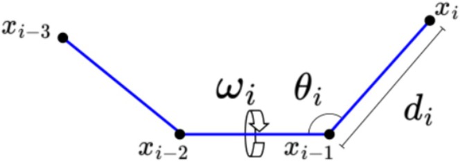 FIGURE 1
| Model | Number of operations |
|---|---|
| Euclidean | |
| Homogeneous | |
| Conformal |
- —Fundação de Amparo à Pesquisa do Estado de São Paulo10.13039/501100001807
- —Conselho Nacional de Desenvolvimento Científico e Tecnológico10.13039/501100003593
Peer Reviews
No public reviews on file for this paper yet. If you reviewed it on a platform where reviews are public (OpenReview, ICLR, NeurIPS, ICML), you can paste yours below so the community can read it here.
Videos
No videos yet. Explain this paper in a talk, walkthrough, or lecture? Add one.
Taxonomy
TopicsCrystallography and molecular interactions · Supramolecular Chemistry and Complexes · Synthesis and Properties of Aromatic Compounds
Introduction
1
In computational chemistry, the geometric arrangement of atoms within a molecule is often represented using Cartesian or internal coordinates (given by the lengths of covalent bonds and the bond and torsion angles), which are particularly useful because they are closely related to the chemical bonds and angles that define the molecule's structure [1].
The traditional approach to converting internal coordinates into Cartesian coordinates involves the use of the homogeneous coordinate system. In this system, each point in 3D space is represented by a vector in ℝ4, allowing for translation and rotation of atoms to be described by matrix operations. This method, as proposed by Thompson in the 1960s [2], has been widely used in molecular geometry calculations (e.g., see [3]).
While the homogeneous coordinate system simplifies the conversion of internal coordinates to Cartesian coordinates, it does not inherently simplify the calculation of interatomic distances, which is a crucial task in molecular geometry optimization and molecular dynamics simulations [4, 5]. To address this limitation, this paper introduces the conformal model for molecular geometry, a generalization of the homogeneous coordinate system [6, 7, 8].
In the conformal model, we define the Conformal Coordinate Matrix (C‐matrix), which allows for a more efficient computation of interatomic distances. The C‐matrix not only retains the advantages of the homogeneous coordinate system but also introduces a new level of computational efficiency by reducing the number of operations required for distance calculations.
This paper explores the mathematical framework of the conformal model, demonstrates its application to molecular geometry, and compares its performance with traditional methods.
Homogeneous Coordinate System
2
Since internal coordinates are naturally associated with the geometry of a molecule, especially when bond lengths and bond angles are considered fixed and given a priori (which reduces the degrees of freedom needed to characterize the 3D structure of a molecule), internal coordinates are widely used in computational chemistry [4] (see Figure 1).
Cartesian and internal coordinates.
We will consider, then (as in Reference [9]), a molecule as a linear chain of n atoms described by internal coordinates di,θi,ωi, where di is the covalent bond length between atoms with Cartesian coordinates xi−1,xi∈ℝ3 (i=2,…,n), θi is the angle formed by the bond vectors bi−1,bi, given by bi=xi−xi−1 (i=3,…,n), and ωi is the torsion angle formed by the planes generated by bi−2,bi−1 and bi−1,bi (i=4,…,n).
In Reference [2] (see also [10]), Thompson proposes using the homogeneous model of 3D space (where each point is represented by (x,y,z,1)t∈ℝ4) to convert internal coordinates into Cartesian coordinates. This approach allows for grouping the three “positioning movements” of an atom (one translation and two rotations), considering previous atoms in the chain, into a single linear operator. As a result, the calculation of Cartesian coordinates from internal coordinates is simply given by a matrix product, as we summarize below following the procedure given in Reference [9].
The rotations associated with the bond and torsion angles are given in the homogeneous space by
respectively, and the translation of a point xi∈ℝ3 is encoded by
Combining these matrices, we get
For d1=ω1=ω2=ω3=0 and θ1=θ2=π, we obtain
and, for i=4,…,n,
where e4=(0,0,0,1)t is the vector in the homogeneous space that represents the “origin” of 3D space.
To simplify the notation, let us write
and calculate the Euclidean distance ri,j between xi and xj (for i<j) (I is the identity matrix):
Although the term B[1,i] is not an orthogonal matrix, the authors in Reference [9] show that it can be removed, resulting in
Conformal Coordinate System
3
To obtain the position of the fourth atom in the molecule,
we first calculate B4e4, using the matrix
In this matrix, we see that the rotations associated with the bond angle θ4 and the torsion angle ω4 are represented by
and the translation associated with the bond length d4 (applied to a unit vector that has already undergone two rotations by the angles θ4 and ω4) is encoded by
In other words, using homogeneous coordinates, the translation (in 3D space) is linearized (in 4D space) and the three operations are represented by a single matrix. This linearization, in general, can be represented by
where x∈ℝ3.
Note that the matrix A, related to the rotations, is orthogonal. However, when we linearize the translation, the new matrix, now in ℝ4×4, is no longer orthogonal.
In Reference [11], the authors manage to “recover” this property (slightly modifying the concept of orthogonality) by using another model of 3D space, called the conformal model [6, 7, 8].
In ℝ3, the two rotations and the translation given in Equation (1) can be represented by a function f:ℝ3→ℝ3, defined by
where A∈ℝ3×3, such that A−1=At, and b∈ℝ3. That is, f is an isometry in ℝ3.
Also in Reference [11], it is demonstrated that it is not possible to “orthogonalize” isometries in 3D space using the homogeneous model. However, by renouncing the positivity of the usual inner product and using the conformal model, one can encode translations in 3D space as orthogonal operations in ℝ5. In that paper, the motivation was the search for an orthogonal representation of isometries in 3D space. Perhaps, due to the chosen notation, the development of this reasoning was not very clear. We present an alternative below, which we believe is more convincing.
Orthogonalization of Isometries
3.1
The entire argument in Reference [11] is based on constructing a bijection between ℝ3 and a subset ℍ⊂ℝ5, in such a way that isometries in ℝ3 can be represented orthogonally in ℝ5. For each x∈ℝ3, its representative in ℍ will be denoted by x^∈ℝ5.
We want that when applying an isometry f:ℝ3→ℝ3 to x,y∈ℝ3, their respective representatives x^,ŷ∈ℍ⊂ℝ5 are altered orthogonally.
In other words, we would like to demonstrate that, for any x,y∈ℝ3,
One way to obtain this result would be to assume that the inner product in ℝ5 “encodes” the Euclidean distance in ℝ3. That is, if
we would have
which would imply
The question, therefore, is to investigate how the hypothesis x^·ŷ=‖x−y‖2, with x,y∈ℝ3 and x^,ŷ∈ℝ5, could lead to the discovery of the bijection in question between ℝ3 and the subset ℍ⊂ℝ5.
So far, we have considered the usual inner product, both in ℝ3 and in ℝ5, which induces Euclidean norms in both spaces.
The first consequence of the hypothesis x^·ŷ=‖x−y‖2 is that, setting x=y, we would have
which would be a contradiction because we are looking for a bijection.
To avoid this contradiction, we will abandon the positivity of the inner product in ℝ5, which implies that (assuming x^·ŷ=‖x−y‖2),
That is, we will admit that all points in 3D space will be represented by vectors in ℝ5 with zero norm. Of course, this norm, induced by the new inner product, will no longer be Euclidean (we will continue to call it “the new inner product”, even though we know that, formally, we no longer have such an operation due to the lack of positivity).
The other properties that define an inner product will be preserved. This means that we will maintain the algebraic properties of the inner product in ℝ5 (symmetry, homogeneity, and distributivity), but as the Euclidean character requires the positivity of the inner product, the geometry in ℝ5 will be altered. Therefore, we are looking for a non‐Euclidean representation (that lies in ℝ5) for the 3D space. By abuse of notation, we will continue writing x^·ŷ to represent the new inner product.
From Reference [11], knowing that it is not possible to orthogonalize isometries of 3D space in ℝ4, even by relinquishing the positivity of the inner product, we can follow what is done in the homogeneous model and represent a point x=x1e1+x2e2+x3e3∈ℝ3 in ℍ⊂ℝ5 by
where x1,x2,x3,x4,x5∈ℝ and, together with e1,e2,e3∈ℝ3, e4,e5 are vectors that complete the canonical basis of ℝ5. Of course, for the above sum to make sense, we add zeros to the fourth and fifth coordinates when embedding x,e1,e2,e3 in ℝ5. The problem now is to determine the values of x4 and x5.
From the algebraic properties of the inner product in ℝ5, we easily obtain that
In other words,
Because the norm in ℝ5 is no longer Euclidean, negative norm, as well as zero norm of a non‐zero vector, is no longer forbidden.
Let us also note that the set {e1,e2,e3,e4,e5} is orthogonal, but no longer orthonormal because we will assume ‖e5‖=−1.
Since the vectors in ℍ⊂ℝ5, which represents the points in 3D space, must have zero norm, we will replace e4,e5 with vectors e0,e∞ that also have zero norm (see [11] for more details), defined by
resulting in
and
With the new basis {e1,e2,e3,e0,e∞}, and given that e0,e∞ are also orthogonal to {e1,e2,e3}, we obtain
with x,y∈ℝ3, x0,x∞∈ℝ, and e0,e∞∈ℝ5.
For x^=ŷ,
and, considering x0=1, we finally obtain
implying that
The expression (3) defines the conformal model [7, 8]. Since e0 represents the “origin” of 3D space (x^=x+e0+0.5‖x‖2⇒0^=e0), the conformal model is also known as the generalized homogeneous model (see [11] for details).
With the bijection between ℝ3 and the subset ℍ⊂ℝ5, defined by (3), our hypothesis becomes true with a slight adjustment. That is, for x,y∈ℝ3,
which, in turn, implies that
Thus, we reach our goal: When applying an isometry f:ℝ3→ℝ3 to x,y∈ℝ3, their respective representatives x^,ŷ∈ℝ5 are altered orthogonally (of course, considering the new inner product in ℝ5, which no longer respects positivity).
Conformal Coordinate Matrix (C‐matrix)
3.2
Using the conformal model, an isometry f:ℝ3→ℝ3,
is then represented by
Because of the orthogonality of the matrix A, we get
which implies that the isometry f can be encoded in matrix form as
where x∈ℝ3 (see details in Reference [11]).
Taking
we have
implying that
We denote this matrix as the Conformal Coordinate Matrix of atom i or simply the C‐matrix of atom i.
The C‐matrix is not orthogonal with respect to the usual inner product, but it is if we consider the new one. That is, it satisfies
as we can see in what follows.
From Equation (2),
which implies that, in matrix format,
where
and I∈ℝ3×3. Considering
we obtain
and, in turn,
for all x,y∈ℝ3.
Thus, U (and, in particular, the C‐matrix) is an orthogonal matrix with respect to the inner product defined by (4).
Finally, we are ready to compute distances using the conformal model.
Computing Distances in the Conformal Coordinate System
4
Since the computation of Cartesian coordinates from internal coordinates (using the conformal model) follows the same procedure performed in the homogeneous space (see Section 2), we have that
where
and
with xi∈ℝ3.
As mentioned earlier, e0 is the representative of the origin of 3D space in the conformal model, playing the role of e4 in the homogeneous model.
Without loss of generality, let us consider i<j. Also defining
and writing
we obtain
and, from Equation (5),
Since x^j·x^i∈ℝ,
which implies
As we know that
we have that the Euclidean distance ri,j between atoms i and j is given by
Comparing this with the expression obtained using the homogeneous model [9], given by
we can see that the simplification obtained is due to the orthogonality of B[i], a consequence of the orthogonality of the C‐matrix (of course, orthogonality in terms of the new inner product in ℝ5). We can conclude this because
Number of Operations for Computing ri,j
4.1
In Reference [9], a comparison was made between the Euclidean and homogeneous models regarding the number of operations (additions and multiplications) required to calculate the interatomic distance ri,j between atoms i and j. As in Reference [9], we will disregard the cost associated with calculating sine and cosine functions, as well as the square root, since they appear in equal numbers in all three models.
To compute ri,j in the conformal model, we need to calculate
First, let us determine separately the cost associated with the vectors e∞tBi+1 and B[i+2,j]e0.
Note that the first of these two vectors is exactly given by the fifth row of Bi+1, which requires only 2 multiplications.
For the second vector, B[i+2,j]e0, we need to calculate the fourth column of the matrix resulting from the product Bi+2Bi+3⋯Bj. We will do this through a sequence of matrix‐vector multiplications, operating from right to left.
The first vector calculated is Bje0, which is given by the fourth column of Bj and requires 5 multiplications, as (di2/2) has already been calculated in the first vector, e∞tBi+1. The sequence of matrix‐vector multiplications is performed such that, for p=i+2,…,j−1, we need to calculate
The cost of determining Bp is 9 multiplications, and the cost of multiplying the matrix Bp by the vector B[p+1,j]e0 is 25 multiplications and 20 additions, totaling 54 operations for each index p.
Disregarding the count of multiplications by 0 and 1, and additions with 0, the product of a matrix Bp and a vector, whose fourth component is always equal to 1, requires 9 multiplications and 10 additions. Along with the 9 operations needed to determine each matrix Bp, computing the vector B[p+1,j]e0 requires 28 operations, for p=i+2,…,j−1. Considering the 5 multiplications to determine Bje0 and the 2 multiplications to determine e∞tB[i+1], we have, so far, 28(j−i−2)+7 operations.
The product between e∞tBi+1 and B[i+2,j]e0 requires 1 multiplication and 2 additions (considering that e∞tBi+1 has two zero entries and one entry equal to one, and that B[i+2,j]e0 has one entry equal to one) and we also have to consider the product of the resulting value by two. Thus, the total number of operations to calculate ri,j, using the conformal model, is
In Table 1, we compare the cost determined here with the cost obtained using the homogeneous and Euclidean models, as given in Reference [9] (note that, to make sense, we assume that j>i+2).
Conclusion
5
The conformal model is a generalization of the homogeneous coordinate system, where 3D space is represented by a subset of ℝ5 with an inner product that no longer respects positivity. Widely used in problems of robotics, physics, and computer graphics [12, 13, 14, 15], this paper applies the conformal model, for the first time (as far as we know), to represent atomic positions and calculate interatomic distances in the context of molecular geometry.
As a result, we define the C‐matrix, which, like the Z‐matrix,1 encodes the geometry of a molecule in terms of internal coordinates. However, while the Z‐matrix is primarily used as a structured representation of molecular configurations, the C‐matrix leverages the conformal model to enable a computationally more efficient calculation of interatomic distances.
Conflicts of Interest
The authors declare no conflicts of interest.
The reference list from the paper itself. Each links out to its DOI / PubMed record.
- 1J. Li , O. Zhang , S. Lee , et al., “Learning Correlations Between Internal Coordinates to Improve 3d Cartesian Coordinates for Proteins,” Journal of Chemical Theory and Computation 19 (2023): 4689–4700.36749957 10.1021/acs.jctc.2c 01270 PMC 10404647 · doi ↗ · pubmed ↗
- 2H. B. Thompson , “Calculation of Cartesian Coordinates and Their Derivatives From Internal Molecular Coordinates,” Journal of Chemical Physics 47 (1967): 3407–3410.
- 3L. Liberti , C. Lavor , N. Maculan , and A. Mucherino , “Euclidean Distance Geometry and Applications,” SIAM Review 56 (2014): 3–69.
- 4J. Parsons , J. Holmes , J. Rojas , J. Tsai , and C. Strauss , “Practical Conversion From Torsion Space to Cartesian Space for In Silico Protein Synthesis,” Journal of Computational Chemistry 26 (2005): 1063–1068.15898109 10.1002/jcc.20237 · doi ↗ · pubmed ↗
- 5V. Rybkin , U. Ekström , and T. Helgaker , “Internal‐To‐Cartesian Back Transformation of Molecular Geometry Steps Using High‐Order Geometric Derivatives,” Journal of Computational Chemistry 34 (2013): 1842–1849.23703109 10.1002/jcc.23327 · doi ↗ · pubmed ↗
- 6A. Dress and T. Havel , “Distance Geometry and Geometric Algebra,” Foundations of Physics 23 (1993): 1357–1374.
- 7D. Hestenes , “Old Wine in New Bottles: A New Algebraic Framework for Computational Geometry,” in Advances in Geometric Algebra With Applications in Science and Engineering, ed. E. Bayro‐Corrochano and G. Sobczyk (Birkhäuser, 2001), 1–14.
- 8H. Li , D. Hestenes , and A. Rockwood , “Generalized Homogeneous Coordinates for Computational Geometry,” in Geometric Computing With Clifford Algebra, ed. G. Sommer (Springer, 2001), 25–58.