Comparing vorticity and curvature Rossby numbers
Chuanyin Wang, Rui Xin Huang, Dake Chen, Qinghua Yang

TL;DR
This paper compares two methods for measuring ocean flow nonlinearity and finds one to be more accurate.
Contribution
The study identifies the curvature Rossby number as a more accurate representation of oceanic flow nonlinearity.
Findings
The vorticity Rossby number overestimates nonlinearity by ignoring kinetic energy variation.
The curvature Rossby number accounts for kinetic energy and provides better accuracy.
Theoretical and data analysis confirm the superiority of the curvature Rossby number.
Abstract
In ocean dynamics, there is often a need to measure the point-by-point significance of the nonlinear term compared with the Coriolis term in the momentum equations. The bulk Rossby number (i.e., UfL) does not meet this need, which necessitates the proposal for the pointwise Rossby number. Conventionally, two different formulations are used to represent the pointwise Rossby number approximately. One is the vorticity Rossby number defined as the ratio of the relative vorticity to the planetary vorticity (i.e., ζf), and the other is the curvature Rossby number formulated as the ratio of the curvature vorticity to the planetary vorticity (i.e., ζcurvf). It remains unknown which approximate representation is more accurate. Here we compare their accuracies on the basis of theoretical and data analysis. The vorticity Rossby number is found to overestimate the pointwise nonlinearity of oceanic…
Click any figure to enlarge with its caption.
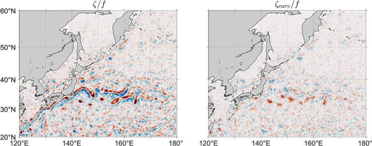 Figure 1
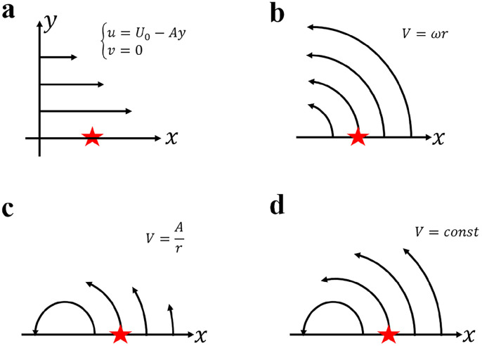 Figure 2
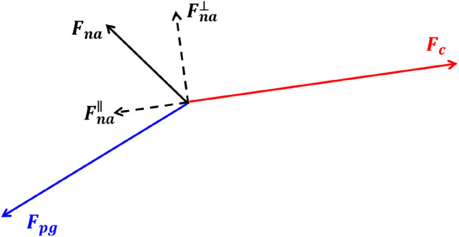 Figure 3
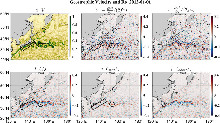 Figure 4
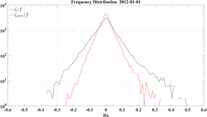 Figure 5
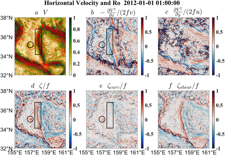 Figure 6
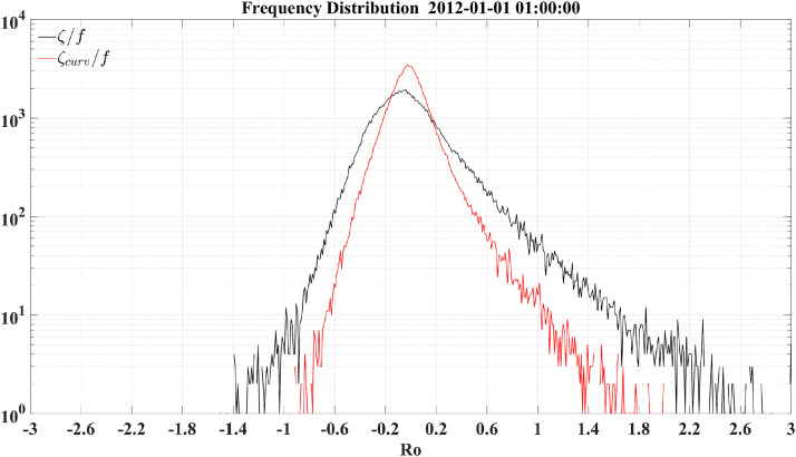 Figure 7
Peer Reviews
No public reviews on file for this paper yet. If you reviewed it on a platform where reviews are public (OpenReview, ICLR, NeurIPS, ICML), you can paste yours below so the community can read it here.
Videos
No videos yet. Explain this paper in a talk, walkthrough, or lecture? Add one.
Taxonomy
TopicsOceanographic and Atmospheric Processes · Geophysics and Gravity Measurements · Ocean Waves and Remote Sensing
Introduction
1
The momentum equations describing the oceanic flow involve many terms, such as the temporal derivative, nonlinear advection, Coriolis acceleration, pressure gradient force and viscosity. Non-dimensional numbers are often introduced to evaluate the importance of one term in comparison with others. For example, in the textbooks of geophysical fluid dynamics [[1], [2], [3]], the relative importance of the advection and Coriolis terms is estimated by the bulk Rossby number Ro_bulk_ , where U, L and f are the characteristic velocity scale, length scale and Coriolis parameter, respectively. When Ro_bulk_ is much smaller than one for a dynamical process (e.g., barotropic tide), the advection term can be neglected and the linear dynamics dominates; when Ro_bulk_ is on the order of one for a certain type of oceanic motion (e.g., submesoscale process), advection and Coriolis terms are comparable so that both terms should be retained; when an oceanic process (e.g., three-dimensional turbulence) is characterized by Ro_bulk_ much larger than one, the Coriolis term is negligible and it is a highly-nonlinear regime. Unfortunately, in practice, it is nontrivial to specify characteristic scales U and L in calculating Ro_bulk_ because the oceanic motion is a nonlinear entanglement of multiple dynamical processes, ranging from the basin scale through the mesoscale to the dissipation scale. Moreover, by definition, Ro_bulk_ is a rough estimate for an oceanic regime rather than an accurate representation of the nonlinearity. Thus, it is very useful for the scale and asymptotic analysis, but it is less useful when there exists the necessity to accurately represent the point-by-point nonlinearity. This necessity is becoming even more pressing with the rapid development in the study aimed at submesoscale processes embedded in the highly variable, multiscale ocean circulation. A pointwise Rossby number is desirable for the local and accurate comparison of the advection and Coriolis terms.
Usually invoked, without any justification, as an approximation of the pointwise Rossby number is the gradient Rossby number , where is the vertical component of the relative vorticity (hereafter referred to as the relative vorticity) and f is also known as the planetary vorticity [4,5]. In this study, the gradient Rossby number is called the vorticity Rossby number, namely Ro_vort_ , for a comparison with the other formulation of the pointwise Rossby number, which will be introduced in the next paragraph. We think that Ro_vort_ is a gradient non-dimensional number that finds its greatest use in the stability analysis (e.g., inertial stability); thus, a large Ro_vort_ does not necessarily imply the significance of the advection term. An insightful example is the turbulent thermal wind, which is a linear horizontal momentum balance among the Coriolis force, baroclinic pressure gradient and vertical momentum mixing [6,7]. For a filament in the turbulent thermal wind balance, Ro_vort_ can reach as large as 5.3 [6,7]. This example demonstrates that Ro_vort_ is not a dynamically accurate approximation of the pointwise Rossby number. One aim of this study is to comprehensively elucidate why this could happen.
Another approximation of the pointwise Rossby number is proposed as , where is the curvature vorticity [[8], [9], [10]]. In this study, we call it the curvature Rossby number, namely Ro_curv_ . Although it has been introduced for a long time, Ro_curv_ receives less attention than does Ro_vort,_ and it remains unclear how accurate Ro_curv_ is, in comparison with Ro_vort_, in measuring the pointwise nonlinearity strength. Our second aim is to show that Ro_curv_ is a better candidate for the pointwise Rossby number.
In Section 2, the vorticity Rossby number is derived from the momentum equations in the Cartesian coordinate system, and its shortcomings are illustrated with the help of idealized flow models. In Section 3, the curvature Rossby number is formulated based on the momentum equations in the natural coordinate system, and its advantages are demonstrated in comparison to the vorticity Rossby number. Section 4 further compares these two Rossby numbers by applying them to the analysis of satellite altimetric observations and high-resolution numerical simulation. Section 5 concludes the paper with a summary and discussion.
Vorticity Rossby number
2
Mathematical derivation
2.1
Consider the rotating shallow-water momentum equations in the Cartesian coordinate system:
where is the x-direction velocity, the y-direction velocity, the acceleration due to gravity and the sea surface height. Let , and . Using the vector identity , the nonlinear advection terms of Eq. 1 can be rewritten into the well-known Gromeka-Lamb form [1,11]:
where is the relative vorticity. Obviously, both the relative vorticity and the spatial inhomogeneity of the kinetic energy contribute to the nonlinearity of the momentum equations. Correspondingly, Eq. 1 becomes:
By definition, the pointwise Rossby number is the ratio of the nonlinear advection term to the Coriolis acceleration term, yielding:
where Ro_x_ and Ro_y_ denote the pointwise Rossby number in x- and y-momentum equations, respectively. It is evident that the vorticity Rossby number Ro_vort_ merely includes the effect of the relative vorticity and neglects the contribution from the spatial variation of the kinetic energy. As a result, the pointwise Rossby number is expected to be significantly misestimated by Ro_vort_ wherever the kinetic energy varies significantly. In the following analysis, four idealized flow models will be used to demonstrate that the kinetic energy term indeed substantially counteracts the effect of the relative vorticity and thus plays an important role in regulating the nonlinearity of the momentum equations (i.e., Eq. 1 or 3).
Idealized flow models
2.2
First, the shear flow (e.g., the Kuroshio, the Antarctic Circumpolar Current) is one of the most common motions in the ocean and deserves particular attention. As shown in Fig. 1a, the velocity profile of the uniform shear flow model is , where U_0_ and A are constant. From Eq. 3, we find that the x-momentum equation is reduced to a trivial identity 0 = 0 at the location denoted by the red pentagram, while the y-momentum equation becomes:
Fig. 1Idealized flow models. Panels (a-d) show the uniform shear flow, uniform circular motion, point vortex, and circular motion with uniform kinetic energy, respectively. The solid lines represent streamlines, with arrows indicating flow directions. The red pentagrams denote the locations under consideration. U_0_ in (a) is a constant flow along the positive x direction, A in (a, c) is a positive constant, V in (b-d) is the flow speed, in (b) is the angular speed, and r in (b, c) is the radial distance.Fig 1
Note that the relative vorticity term (i.e., the first term on the left-hand side of Eq. 5a) exactly cancels the kinetic energy term (i.e., the second term on the left-hand side of Eq. 5a). As a result, the nonlinear advection term vanishes and the simple geostrophic balance is obtained. Correspondingly, Ro_x_ in Eq. 4 is ill-defined because each term of the x-momentum equation is identically zero, and the y-direction pointwise Rossby number becomes:
Eq. 6 indicates a simple fact that the geostrophic balance has a vanishing pointwise Rossby number. In striking contrast, the vorticity Rossby number Ro_vort_ is non-zero and is thus unable to correctly represent the pointwise nonlinearity of the momentum equations for uniform shear flows owing to the neglect of the kinetic energy term whose effect is to cancel the contribution of the relative vorticity term.
Second, the uniform circular motion (Fig. 1b) is considered because the real ocean is ubiquitously populated by vortex motions, and the mesoscale vortex circulates approximately as a rigid body [12]. The analytic velocity expression for this idealized flow model is , where is the flow speed, the angular speed, and r the radial distance. At the specific point denoted by the red pentagram, the y-momentum equation is identically satisfied, and this could be readily justified by introducing the polar coordinate system and substituting the velocity profile; then the x-momentum equation is:
Eq. 7b shows that half of the relative vorticity term is cancelled by the kinetic energy term, and the other half contributes to the centripetal acceleration, which results in the gradient wind balance. Correspondingly, the x-direction pointwise Rossby number in Eq. 4 becomes:
By contrast, the vorticity Rossby number is Ro_vort_ and gives an overestimate by a factor of 2 due to neglecting the effect of the kinetic energy term.
Third, the irrotational motion is worth being considered for the theoretical clarity. An example is the point vortex (Fig. 1c), whose relative vorticity is zero everywhere except for the singular point at the origin. For the point vortex model, the analytic velocity expression is . Similar to the uniform circular motion, only the x-momentum equation is present at the specific point denoted by the red pentagram
Eq. 9b shows the gradient wind balance as in the last case, but here the centripetal acceleration is completely attributed to the kinetic energy term due to the absence of the relative vorticity term. Corresponding to Eq. 9b, the x-direction Rossby number is:
Evidently, the vorticity Rossby number Ro_vort_ completely misrepresents the pointwise nonlinearity of the momentum equations in this case because of the neglect of the kinetic energy term.
Lastly, let us consider the special scenario where the kinetic energy is spatially uniform. Take, for instance, an idealized circular flow model with uniform kinetic energy (Fig. 1d). The momentum equations (i.e., Eq. 3) become:
The nonlinearity of Eq. 11 is completely determined by the relative vorticity term. Consequently, the pointwise Rossby numbers are totally explained by the relative vorticity as follows:
Therefore, for the uniform-kinetic-energy circular flow, the vorticity Rossby number is perfectly exact in weighing the pointwise strength of the nonlinear advection term relative to the Coriolis acceleration. Unfortunately, this kind of flow seldom exists in the real ocean.
Short remark
2.3
It has been demonstrated in Sections 2.1-2.2 that the vorticity Rossby number fails to include the contribution of the kinetic energy term, which acts to counterbalance the relative vorticity term and is thus an incomplete measure for the relative strength of the advection and Coriolis terms. It is necessary to find an improved approximation of the pointwise Rossby number. At first sight, the simplest way of improvement appears to be retaining the kinetic energy term, namely directly utilizing Ro_x_ and Ro_y_ in Eq. 4 as a measure of the pointwise Rossby number. However, Ro_x_ (Ro_y_) could become singular and incapable of providing an accurate description wherever the meridional (zonal) velocity is zero, and thus the Coriolis force vanishes. Instead of the conventional Cartesian coordinate, the natural coordinate system can be used to avoid such a singular case, which leads to the curvature Rossby number in Section 3.
Curvature Rossby number
3
Mathematical derivation
3.1
Consider the rotating shallow-water momentum equations in the natural coordinate system [4]:
where s (s) is the distance (unit vector) along the streamline, n (n) the distance (unit vector) perpendicular to the streamline, α the angular direction of the flow velocity and the curvature vorticity with R_s_ denoting the radius of the streamline curvature. Recall that the sum of the curvature vorticity and shear vorticity is equal to the relative vorticity [13,14]. It is important to note that the Coriolis force is only present in the direction perpendicular to the streamline and that the nonlinear term along that direction is exactly the curvature vorticity term in contrast to the Cartesian formulation (i.e., Eq. 4) where the relative vorticity term only partially represents the nonlinearity. Therefore, it is straightforward to formulate the pointwise Rossby number in the direction perpendicular to the streamline by calculating the ratio of the second to third terms on the left-hand side of Eq. 13b, obtaining:
As mentioned in Section 1, this formulation has been previously proposed and is here called the curvature Rossby number. Mathematically, Ro_curv_ avoids the singularity induced by vanishing meridional or zonal velocity.
It is argued that Ro_curv_ is an intrinsic description of the flow nonlinearity. For a physical explanation, let us invoke an argument that is independent of the coordinate system. Fig. 2 shows a balance among the Coriolis acceleration (i.e., Where )) perpendicular to the streamline, pressure gradient (i.e., ) and nonlinear acceleration (i.e., ). Two components of are and , which are respectively parallel and perpendicular to . When is used as a reference to weigh the importance of , it is precisely that is compared with . It is readily proven that is exactly equal to:
Ro_curv_ is exactly the ratio which is independent of the choice of the coordinate system and thus intrinsically measures the relative significance of the nonlinear acceleration and Coriolis force. It is also obvious from the derivation in Eq. 15 that the shear vorticity component of the relative vorticity term is completely cancelled by the kinetic energy term; consequently, the shear vorticity does not contribute to the nonlinearity of the momentum equation in the direction parallel to the Coriolis acceleration. Therefore, Ro_curv_ correctly removes the spurious influence of the shear vorticity through recovering the kinetic energy term, while Ro_vort_ redundantly includes the contribution of the shear vorticity due to the neglect of the kinetic energy term. Incidentally, it is unreasonable to weigh against since they are completely misaligned. To determine the relative strength of , another reference term, such as the pressure gradient force along the streamline, can be used. But that is irrelevant to the formulation of the pointwise Rossby number and thus beyond the scope of this study.Fig. 2A balance among the Coriolis acceleration , pressure gradient and nonlinear acceleration . ( ) is the component of parallel (perpendicular) to **.**Fig 2
To summarize, Ro_curv_ is superior in describing the pointwise nonlinearity strength relative to the Coriolis force, which will be further illustrated by idealized flow models in the following.
Idealized flow models
3.2
Table 1 shows the vorticity Rossby number Ro_vort_ and the curvature Rossby number Ro_curv_ for the four idealized flow models whose exact pointwise Rossby numbers (i.e., Ro_x_ or/and Ro_y_) at the red-pentagram points (Fig. 1) are known a priori. As also detailed in Section 2, Ro_vort_ completely misrepresents the pointwise Rossby number for the typical oceanic shear flow with zero curvature vorticity but non-zero shear vorticity and it overestimates the nonlinearity of the typical oceanic vortex whose shear vorticity and curvature vorticity are of the same sign, which holds regardless of the vortex polarity and hemisphere. Only for the uniform-kinetic-energy circular flow whose shear vorticity vanishes, Ro_vort_ correctly reproduces the pointwise Rossby number. By contrast, Ro_curv_ faithfully recovers Ro_x_ or/and Ro_y_ for all idealized flow models.Table 1Rossby numbers for the four idealized flow models.Table 1. Uniform shear flowUniform circular flowPoint vortexUniform kinetic energy flowRo_x_**Ro_x_ is ill-defined Ro_y_ Ro_y_ is ill-defined**Ro_y_ is ill-defined Ro_vort_ 0 Ro_curv_0 Note that for the uniform kinetic energy flow.
Quasi-realistic application
4
With the mathematical derivation and idealized flow models having provided solid evidence in 2, 2.1, we now proceed with the quasi-realistic cases. First, the gridded geostrophic velocity data are used to compare the vorticity and curvature Rossby numbers. The data are derived from sea surface height observations by the nadir-looking satellites and provided by the Copernicus Marine Service. The spatial resolution of the data is 1/4^°^, and thus large-scale motions are well captured, and mesoscale processes are partially resolved. Fig. 3 shows the comparison around the Kuroshio and its extension, a region characterized by shear flows (e.g., the black box in Fig. 3a) and mesoscale vortices (e.g., the solid and dashed circles in Fig. 3a, respectively). The vorticity Rossby number Ro_vort_ (Fig. 3d) has large magnitudes along the shear flow and inside vortices, while the kinetic energy terms (Fig. 3b, c) tend to have a counteracting effect, especially along the shear flow. Note that the distribution of the kinetic energy term has a patchy structure of extremely large/small values resulting from the nearly vanishing meridional or zonal velocity. These singular points indicate that, as argued in Section 2, a direct inclusion of the kinetic energy term into the vorticity Rossby number is not the proper way to improve the representation of the pointwise Rossby number. On the other hand, the curvature Rossby number Ro_curv_ (Fig. 3e), correctly excluding the contribution of the shear vorticity (Fig. 3f), especially along the shear flow and inside vortices, is generally smaller in magnitude. This is more clearly shown by the histograms of Ro_vort_ and Ro_curv_ in Fig. 4, with the former displaying a wider distribution than the latter. Such an overestimate of the nonlinearity by Ro_vort_ is understandable since the shear vorticity tends to be of the same sign as the curvature vorticity, as obviously seen in the case of the oceanic mesoscale vortex. The vanishingly small Ro_curv_ along the shear flow and decreased Ro_curv_ inside mesoscale vortices agree with the basic observations from idealized flow models in Section 3.2. In addition to the magnitude overestimate, the standard deviation of Ro_curv_ (i.e., 0.042) is 42% smaller than that of Ro_vort_ (i.e., 0.072), indicating that the distribution patterns of the two Rossby numbers are also strikingly different.Fig. 3The satellite-altimeter-based flow speed (a), the ratio of thex**-derivative of the kinetic energy to thex-direction Coriolis acceleration (b), the ratio of they-derivative of the kinetic energy to they-direction Coriolis acceleration (c), the ratio of the relative vorticity to the planetary vorticity (d), the ratio of the curvature vorticity to the planetary vorticity (e) and the ratio of the shear vorticity to the planetary vorticity (f) around the Kuroshio and its extension.** The black boxes, black solid circles and black dashed circles highlight a shear flow, a cyclonic vortex and an anticyclonic vortex, respectively.Fig 3. Fig. 4The satellite-altimeter-based frequency distribution of the Rossby numbers. The black and red curves denote the vorticity and curvature Rossby numbers, respectively. Note that a logarithmic scale is used for the y axis.Fig 4
Since nadir-looking satellite altimetry cannot well resolve submesoscale flows and the internal gravity wave continuum, a realistic numerical simulation (i.e., LLC4320) is employed to further demonstrate the advantages of the curvature Rossby number. Simultaneously forced by atmospheric fields and tidal potentials, the LLC4320 simulation has a spatial resolution of ∼2 km and outputs hourly snapshot variables. This simulation can reproduce not only large-scale currents and mesoscale variabilities [15,16] but also submesoscale flows and internal gravity waves [[17], [18], [19]], mimicking the real ocean with multiscale dynamical processes. We focus on a section of the Kuroshio Extension (Fig. 5), especially on a shear flow (black boxes) and a cyclonic vortex (black circles). According to the vorticity Rossby number Ro_vort_ (Fig. 5d), the shear flow and the eddy display seemingly strong nonlinearity, which is, however, counteracted by the kinetic energy term (Fig. 5b-c). This is consistent with the conclusion from the idealized flow model in Section 2.2 and the satellite observation in Fig. 3. Again, the kinetic energy term should not be directly added to estimate the pointwise Rossby number because of its unreasonably high/low values resulting from velocity singularity. By contrast, the curvature Rossby number Ro_curv_ (Fig. 5e) excludes the spurious contribution of the shear vorticity (Fig. 5f) contained in the vorticity Rossby number Ro_vort_, and thus correctly exhibits a much smaller magnitude than Ro_vort_, which is also evident in the histograms of Ro_vort_ and Ro_curv_ (Fig. 6). Thus Ro_curv_ presents a nearly negligible nonlinearity for the shear flow and a much weaker nonlinearity for the cyclonic vortex shown in Fig. 5, which agrees with the results from the uniform shear flow and the uniform circular flow in Section 3.2. In addition to the obvious difference in the magnitude, Ro_curv_ and Ro_vort_ also show quite distinct distribution patterns, as demonstrated by their contrasting standard deviations (0.202 for Ro_curv_ and 0.348 for Ro_vort_).Fig. 5The LLC4320 flow velocity and speed (a), the ratio of thex**-derivative of the kinetic energy to thex-direction Coriolis acceleration (b), the ratio of they-derivative of the kinetic energy to they-direction Coriolis acceleration (c), the ratio of the relative vorticity to the planetary vorticity (d), the ratio of the curvature vorticity to the planetary vorticity (e) and the ratio of the shear vorticity to the planetary vorticity (f) around the Kuroshio Extension.** The black boxes and circles highlight a shear flow and a cyclonic vortex, respectively.Fig 5. Fig. 6The LLC4320-based frequency distribution of the Rossby numbers. The black and red curves denote the vorticity and curvature Rossby numbers, respectively. Note that a logarithmic scale is used for the y axis.Fig 6
Summary and discussion
5
This short study revisits two approximate formulations of pointwise Rossby numbers, largely motivated by the recent attention on submesoscale processes where the nonlinearity is strong and comparable to the effect of the Earth's rotation. Most often, the pointwise Rossby number is approximated by the vorticity Rossby number, which is the ratio of the relative vorticity to the planetary vorticity. The vorticity Rossby number fails to include the effect of the kinetic energy term, as seen when the momentum equations are presented in the Gromeka-Lamb form. Using idealized flow models, it is demonstrated that the kinetic energy term is an important contributor to the nonlinearity and definitely non-negligible. As an alternative, the curvature Rossby number was previously proposed as the ratio of the curvature vorticity to the planetary vorticity and, by construction, serves as a better candidate for the pointwise Rossby number owing to the recovery of the kinetic energy term. The application to idealized flow models and quasi-realistic oceanic data further confirms that the curvature Rossby number is a more faithful representation of the relative magnitude of the nonlinear advection and the Coriolis force, while the vorticity Rossby number redundantly includes the contribution of the shear vorticity and thus significantly overestimates the pointwise nonlinearity of the momentum equations. In particular, the curvature Rossby number correctly estimates the pointwise Rossby number of the uniform shear flow to be zero while the vorticity Rossby number gives a complete misrepresentation; the curvature Rossby number accurately estimates the pointwise Rossby number of the idealized oceanic vortex while the vorticity Rossby number formulation gives an overestimate by a factor of 2. It is expected that the curvature Rossby number, which represents a perspective from the natural coordinate system, will help us to diagnose and understand the multiscale ocean dynamics in general and the highly-nonlinear submesoscale processes in particular. Coincidentally, ocean dynamics in the natural coordinate system has recently attracted much attention and revealed illuminating insights into the cyclogeostrophic adjustment and frontogenesis of a curved front [20], the Ekman transport and pumping in a curved balanced flow [21], the symmetric instability of a curved front [22,23], etc. It seems that the curved ocean dynamics merits more future explorations.
Data availability statement
The satellite altimeter data can be downloaded from https://data.marine.copernicus.eu/product/SEALEVEL_GLO_PHY_L4_MY_008_047/description. The LLC4320 simulation outputs are available at https://data.nas.nasa.gov/ecco/data.php?dir=/eccodata/llc_4320. The code to calculate the curvature Rossby number is available at https://doi.org/10.5281/zenodo.10578948.
Declaration of competing interest
The authors declare that they have no conflicts of interest in this work.
The reference list from the paper itself. Each links out to its DOI / PubMed record.
- 1Pedlosky J.Geophysical fluid dynamicssecond ed.1987 Springer New York
- 2Gill A.Atmosphere-ocean dynamics 1982 Academic Press New York
- 3Vallis G.Atmospheric and ocean fluid dynamics: Fundamentals and large-scale circulation 2006 Cambridge University Press New York
- 4Thomas L.Tandon A.Mahadevan A.Submesoscale processes and dynamics Hecht M.W.Hasumi H.Ocean modeling in an eddying regime 2008 American Geophysical Union Washington, DC 1738
- 5Su Z.Wang J.Klein P.Ocean submesoscales as a key component of the global heat budget Nat. Commun.9120187752947258610.1038/s 41467-018-02983-w PMC 5823912 · doi ↗ · pubmed ↗
- 6Gula J.Molemaker M.J.C.Mc Williams J.Submesoscale cold filaments in the Gulf Stream J. Phys. Oceanogr.4410201426172643
- 7Mc Williams J.C.Gula J.Molemaker M.J.Filament frontogenesis by boundary layer turbulence J. Phys. Oceanogr.458201519882005
- 8Knauss J.A.Introduction to physical oceanographysecond ed.1996 Waveland Press Inc., Long Grove