Enhancing EEG Decoding with Selective Augmentation Integration
Jianbin Ye, Yanjie Sun, Man Xiao, Bo Liu, Kele Xu

TL;DR
This paper introduces a new framework and neural architecture to improve EEG analysis using selective data augmentation and contrastive learning, achieving significant performance gains.
Contribution
The novel contribution is an end-to-end EEG augmentation framework with adaptive contrastive learning and a new neural architecture called NeuroBrain.
Findings
The proposed framework achieved a 29.42% performance gain over HappyQuokka.
It showed a 5.45% accuracy improvement compared to EEGNet on EEG decoding tasks.
Abstract
Deep learning holds considerable promise for electroencephalography (EEG) analysis but faces challenges due to scarce and noisy EEG data, and the limited generality of existing data augmentation techniques. To address these issues, we propose an end-to-end EEG augmentation framework with an adaptive mechanism. This approach utilizes contrastive learning to mitigate representational distortions caused by augmentation, thereby strengthening the encoder’s feature learning. A selective augmentation strategy is further incorporated to dynamically determine optimal augmentation combinations based on performance. We also introduce NeuroBrain, a novel neural architecture specifically designed for auditory EEG decoding. It effectively captures both local and global dependencies within EEG signals. Comprehensive evaluations on the SparrKULee and WithMe datasets confirm the superiority of our…
Click any figure to enlarge with its caption.
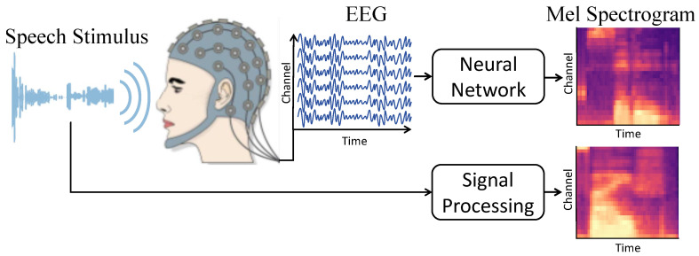 Figure 1
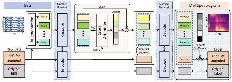 Figure 2
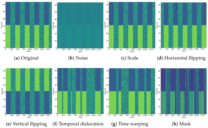 Figure 3
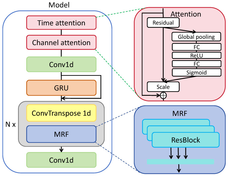 Figure 4
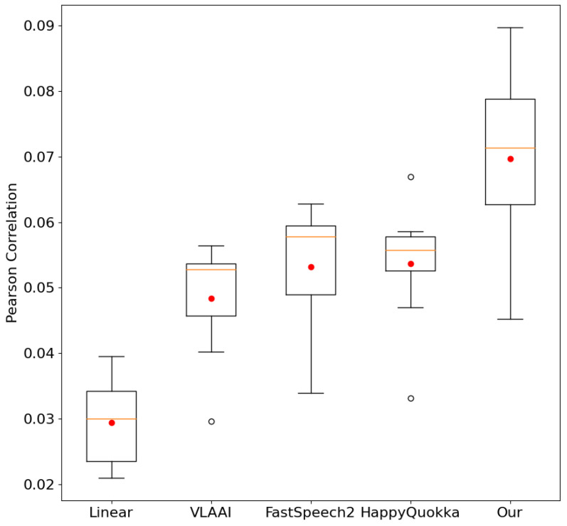 Figure 5
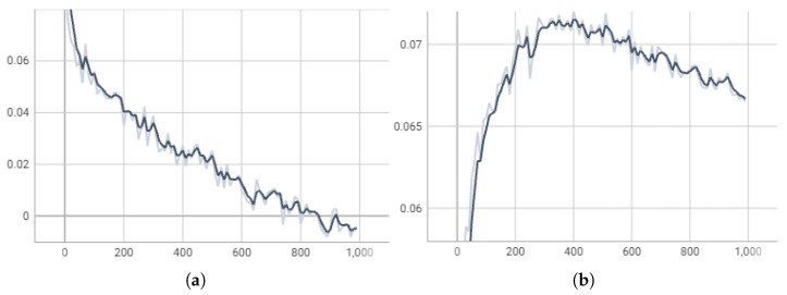 Figure 6
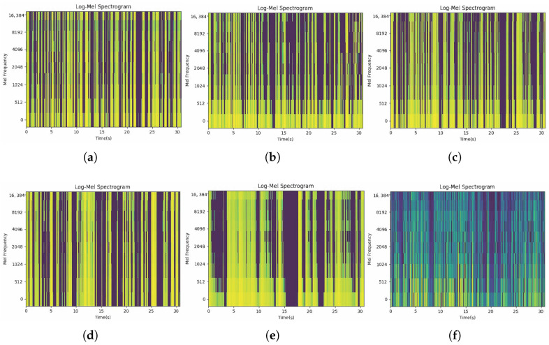 Figure 7
Peer Reviews
No public reviews on file for this paper yet. If you reviewed it on a platform where reviews are public (OpenReview, ICLR, NeurIPS, ICML), you can paste yours below so the community can read it here.
Videos
No videos yet. Explain this paper in a talk, walkthrough, or lecture? Add one.
Taxonomy
TopicsEEG and Brain-Computer Interfaces · ECG Monitoring and Analysis · Neural dynamics and brain function
1. Introduction
Electroencephalography (EEG) signal analysis is a critical area of neuroscience that focuses on studying the brain’s electrical activity as recorded by electrodes placed on the scalp [1,2,3]. EEG plays a dual role in clinical diagnostics and cognitive research, offering valuable insights into neurological functions and disorders. In the clinical domain, EEG is widely recognized for its ability to diagnose conditions such as epilepsy, sleep disorders, and traumatic brain injuries, providing essential information for real-time monitoring and evaluation. Beyond medical applications, EEG has become integral to brain–computer interfaces (BCIs), enabling interaction between users and devices through brain signals, thus driving advancements in assistive technologies and rehabilitation methodologies. As a non-invasive neuroimaging technique, EEG captures cerebral electrical patterns that are indispensable for understanding complex brain activities. The analysis of EEG signals has inspired and continues to benefit from a broad range of methodological advancements across neuroscience [4,5,6,7], signal processing [8,9], and data analysis [10].
EEG auditory decoding is a related research field that aims to decode the features of speech stimuli from EEG. This is achieved by presenting participants with speech while recording an EEG. In this realm, researchers have delved into the intricate, nonlinear relationships between neural activity and observable behaviors, employing machine learning techniques [11,12,13,14,15,16]. These works underscore the versatile applications of EEG in both academic research and practical implementations. Figure 1 demonstrates a conventional EEG auditory decoding procedure, wherein the EEG signals are recorded concurrently with auditory or visual stimuli, followed by the decoding of these signals through diverse decoders.
However, traditional machine learning techniques often encounter difficulties with the high noise levels and temporal variability inherent in EEG signals, necessitating expert oversight for data preprocessing and parameter configuration. Recent advances in deep learning have leveraged its enhanced nonlinear modeling capabilities, facilitating an end-to-end learning approach. For example, Borsdorf et al. [17] make use of a multi-attention mechanism and a gated recurrent neural network to model the temporal dynamics of the EEG signal. Faghihi et al. [18] use a spiking neural network to decode the EEG signals to detect auditory spatial attention. Cai et al. [19] further utilize the spiking graph neural network to capture the dynamic connection between EEG channels. However, this approach’s reliance on fully supervised learning models presents notable constraints. Predominantly, in a conventional fully supervised setting, models are tailored from the ground up for each subject, culminating in a highly individual-specific knowledge base that hampers generalization to new subjects. Furthermore, the efficacy of fully supervised learning heavily depends on the availability of large and high-quality human-annotated datasets. A paucity of such data often leads to diminished model performance, especially within intricate neural network frameworks and novel individuals, thereby compounding the difficulty in crafting versatile and efficient EEG decoding mechanisms.
To address these challenges, we pivot towards self-supervised learning (SSL) as a potent solution. This approach leverages unlabeled data to pre-train deep neural networks, utilizing inherent data features to imbue the model with broader, more generalized knowledge. This foundational training phase is subsequently refined through fine-tuning with a labeled dataset, allowing the network to adjust and improve its performance based on specific, labeled examples. This approach harnesses the vast availability of unlabeled data, enabling more efficient and effective model training by initially learning from the data’s intrinsic patterns before applying targeted adjustments using a smaller set of labeled data. Prior studies have highlighted that self-supervised techniques enhance model robustness and diminish uncertainty [20]. Despite its success in image processing, the adoption of SSL in biosignal processing is less explored, especially in EEG analysis. Initial endeavors in this direction have explored the utilization of diverse augmentation strategies to pre-train encoders to recognize augmented signals, subsequently applying partial or full fine-tuning with labeled data [21,22,23,24,25,26]. While these approaches have yielded promising results, the effectiveness of different augmentation techniques varies across different network architectures and EEG decoding tasks, with some combinations potentially being counterproductive. This observation inspires a novel proposition: could we devise an end-to-end adaptive augmentation method? Such a framework would leverage contrastive learning to bolster the encoder’s representational capacity while autonomously selecting the most effective augmentation combination, thereby maximizing performance.
This paper introduces an end-to-end framework for adaptive augmentation selection, capable of autonomously selecting the optimal augmentation strategies for varying models and tasks. Moreover, we present NeuroBrain, a novel model designed to better effectively decode EEG signals. Our contributions can be summarized as follows:
- We introduce a novel end-to-end framework featuring an adaptive mechanism for the selection of augmentation combinations, specifically engineered for EEG auditory decoding. This innovation facilitates the autonomous determination of the efficacious augmentation strategies across diverse models and tasks.
- To enhance the efficiency of single-model EEG decoding, we introduce NeuroBrain. This model dynamically refines the representation of EEG channels and temporal patterns through an attention mechanism. Combined with a multi-receptive field (MRF) fusion module, it more effectively captures local and global dynamics, leading to improved capabilities in decoding EEG information for both reconstruction and classification tasks.
- Our methodology demonstrates superior performance on two benchmark EEG decoding tasks: SparrKULee for signal reconstruction and WithMe for signal classification. Notably, it surpasses conventional baseline models in both scenarios involving the same subjects (within-subject) and new subjects (unseen-subject), highlighting its effectiveness and generalizability in EEG signal analysis.
The remainder of this paper is organized as follows: Section 2 provides a review of the related literature to contextualize our work within the existing research landscape. Section 3 delineates the proposed methodology in detail. The evaluation of our method, inclusive of a visualization analysis and ablation study, is presented in Section 4. Finally, Section 5 encapsulates a summary and conclusion of this study.
2. Background
2.1. Auditory EEG Decoding
Auditory EEG decoding techniques aim to decode auditory information from EEG signals, providing a new means of human communication via brain signals. Several studies [9,11,27,28,29,30] have proposed various methods and networks. Pallenberg et al. [31] developed a long short-term memory-based neural network architecture that accurately detects the speaker the person is paying attention to. Lee et al. [32] proposed an automatic speech recognition decoder that contributes to decomposing the phonemes of generated speech, thereby displaying the potential of voice reconstruction from unseen words. Dyck et al. [33] introduced a WaveNet-based model that achieved second place in the Auditory EEG Challenge, demonstrating the effectiveness of their network architecture and training strategies. Fu et al. [34] proposed a novel convolutional recurrent neural network for auditory EEG decoding, outperforming linear and state-of-the-art DNN models. Song et al. [35] introduced a compact Convolutional Transformer called EEG Conformer, which achieved state-of-the-art performance and has great potential as a new baseline for general EEG decoding. Thornton et al. [36] focused on the match–mismatch subtask, classifying which speech segment aligned with the EEG signals, and proposed a solution using short temporal EEG recordings. Sun et al. [30] introduced the concept of delay learning [37], which explicitly incorporates the temporal delay between a stimulus and its corresponding EEG pattern. This enhancement significantly improved performance by aligning the EEG signals more precisely with the associated stimuli.
Our research aims to enhance auditory EEG decoding by innovatively applying self-supervised learning techniques, while the primary network architecture is based on the encoder–decoder model.
2.2. Self-Supervised Learning for EEG
Self-supervised learning has been widely used in many fields [38,39,40,41]. In natural language processing, self-supervised models like BERT (Bidirectional Encoder Representation from Transformers) [42] can be well applied to language modeling tasks. In computer vision, self-supervised models like MAE (Masked Autoencoders) [43] can be applied to image representation learning. In the EEG signal processing field, some endeavors have been made. He et al. [44] proposed a self-supervised learning-based channel attention MLP-Mixer network for motor imagery (MI) decoding with EEG, which effectively learned long-range temporal information and global spatial features. Ma et al. [45] introduced a self-supervised learning CNN with an attention mechanism for MI-EEG decoding, demonstrating that learning temporal dependencies improved performance. Wang et al. [46] developed an end-to-end EEG decoding algorithm using a low-rank weight matrix and principled sparse Bayesian learning, achieving improved performance under a self-supervised framework. Partovi et al. [47] proposed a self-supervised deep learning architecture that learned a common vector representation of EEG signals, successfully distinguishing binary classes in different BCI tasks. Song et al. [48] demonstrated the feasibility of learning image representations from EEG signals using a self-supervised framework, with attention modules capturing spatial correlations. Acknowledging the validity of self-supervised learning, we innovatively apply it to address challenges in auditory EEG decoding.
2.3. EEG Signal Augmentations
Various data augmentation techniques have been proposed to generate additional training samples for EEG-based applications. Bhaskarachary et al. [49] explored using machine learning models for EEG preprocessing, feature extraction, and classification to diagnose autism spectrum disorder (ASD). Liu et al. [50] proposed a spatial–temporal data augmentation scheme for brain disorder classification and analysis. Jiang et al. [22] designed various augmentations, including noise addition and affine transformation, which achieve competitive performance on sleep staging tasks. In the EEG-based emotion recognition task, various data augmentation methods have been proposed [21,23,25], which achieved satisfactory emotion recognition performance. We adopted the above method in our work.
However, the above augmentations share a familiar obstacle: implementing comprehensive augmentation policies requires costly manual design and combined efforts. To address this obstacle, Cu-buk [51] presented the AutoAugment algorithm in a computer, which uses reinforcement learning to discover transformations and parameters for data augmentation. This algorithm automatically looks for a suitable data augmentation policy. However, some improvements have been proposed due to the high computational costs and limitations of offline searching in AutoAugment. For instance, Lim [52] uses Bayesian optimization instead of reinforcement learning to reduce the computational burden. Inspired by Lim’s work, we utilize Bayesian optimization to speed up the search process. PBA [53] introduces the concept of population thinking and uses genetic algorithms to find the best strategy from a set of data augmentation strategies. This method achieves dynamic updating of augmentation strategies and continuously optimizes model performance. Lin [54] proposes trainable data augmentation strategy parameters and uses gradient-based optimization to overcome the limitations of offline searching. This method dynamically updates the strategy during training based on model feedback and performs well. Hataya et al. [55] propose Faster AutoAugment, which uses automatic differentiation techniques to search for data augmentation strategies during training. This method achieves efficient augmentation by learning the algorithm to search for augmentation strategies, allowing the learned strategies to be shared and updated throughout the training process. Sun et al. [56] proposed Audio Automatic Augmentation, which extends the AutoAugment method to the audio signal field. Ref. [57] proposes a proxy learning curve for the Bayes classifier for estimation of the minimum training sample size for a required performance. However, there is a lack of research on designing suitable augmentations for the EEG signal. Our research represents the first attempt to develop automatic methods for enhancing EEG signals, significantly improving auditory EEG decoding performance.
3. Methodology
3.1. Overview of Framework
The schematic of our proposed EEG augmentation framework is illustrated in Figure 2, encompassing three stages: (1) augmentation for EEG signal to form enhanced embedding, (2) self-supervised learning with enhanced embedding, and (3) augmentation integration selection. Firstly, to address the issue of insufficient and inherent interference of EEG data, we conducted data augmentation on a subset of the EEG dataset. The raw EEG data is segregated into two streams. The original part is directly routed to the encoder and decoder without additional processing, while the other part undergoes data augmentation, which is illustrated in Section 3.1.1. The EEG signal is enhanced by each augmentation technique, and then, the enhanced EEG signals are delivered to the encoder. A Siamese network [58] is introduced by delivering enhanced EEG data and original EEG data to the encoder/decoder. The encoder in the Siamese network assimilates the representation of both the enhanced and original data. Secondly, given two kinds of feature representation, the embedding after augmentation followed by the encoder should be aligned to the embedding from raw data. After obtaining the weights of the feature map, we protrude the area they look like and pay less attention to the different parts that may be produced by noise signals. Expecting that enhanced embedding is similar to raw embedding as much as possible, we adopt contrast learning here to pull them closer, which is mentioned in Section 3.1.2. Although SSL tries to align various enhanced features, it is still a challenge to bond stylized augmentation techniques. Aiming at the mutual exclusion problem of augmentation techniques, in Section 3.1.3, we designed a selective augmentation integration strategy to adaptively search for the best integration policy of data augmentation methods during training. With negative Pearson correlation loss backward propagating, the importance of a certain integration is reflected by a set of trainable coefficients. According to the importance coefficient of these enhanced outputs, we remove worse outputs and retrain again with new augmentation integration.
3.1.1. Data Augmentation Techniques
Since the collected EEG signals are easily disturbed by ambient noise and the subject’s irregular brain activity is unrelated to the experiment, and the acquisition cost is high, it is necessary to perform data augmentation to make the model learn the characteristics of EEG signals such as time, noise, and other dimensions, improving the robustness of the model. In our training framework, we incorporate seven signal transformation methods that are commonly used in prior research [21,23,25], which are visualized in Figure 3 and described below.
Noise: A random noise segment is collected from the Gaussian distribution and added to the EEG signal.Scale: We perform a range of amplifications or reductions in the amplitude of the EEG signal. The scaled range is constrained from 0.5 to 2.Horizontal flipping: We perform a horizontal flip of two-dimensional EEG data along an intermediate time point, which is equivalent to putting the EEG data in reverse order.Vertical flipping: We perform a vertical flip of two-dimensional EEG data along an intermediate channel, which is equivalent to reversing the EEG data on the channel dimension.Temporal dislocation: We divide the EEG signal into 10 equal-length segments in order of timeline and then randomly shuffle these segments and reassemble them.Time warping: We divide the EEG signal into 10 segments of equal length according to the order of the timeline and then randomly select half of the segments to stretch in the time dimension and the other half to telescope in the time dimension. In this paper, the strength of the stretch is between 1.5 and 2 while the telescoping ranges from 0.5 to 0.67.Mask: A random subset of EEG signal is masked out and replaced by mask tokens initialized by zeros. In this paper, the masking ratio is 30%, leaving 36,864 out of 122,880 (1920 × 64) data points.
3.1.2. Self-Supervised Learning
Data augmentation endows EEG signals with a variety of manifestations, improving the robustness of the encoder. But, for the decoder, multiple kinds of feature maps from the same EEG signal should lead to the same output. Misalignment of the feature map may lead to an inexact reconstructed result. Thus, we utilize contrast learning to make the embedding from the enhanced EEG signal similar to the embedding from the original one. Followed by CLIP [59], a contrast learning loss is computed for each pair of embedding. We assume that there are n participating augmentation methods and every augmentation method corresponds to one embedding , which composites with the original embedding as a pair. Then, a scaled pairwise cosine similarity is computed as follows:
where is a trainable temperature parameter controlling the range of . Given the similarity of the two embeddings, the contrast loss can be obtained by
Let L be the cross entropy loss function and K be a list of , where k is equal to the length of . After that, we obtain an average contrast loss from n pairs of embedding by
3.1.3. Selective Augmentation Integration
Data augmentation techniques for EEG signal described in Section 3.1.1 are beneficial to the robustness and generalization of the EEG decoder. However, applying all augmentation techniques is not fit for all models leading to worse performance. To this end, we propose selective augmentation integration, which is an adaptive training paradigm by updating the augmentation integration policy.
Algorithm 1 illustrates the selective augmentation integration process, which includes two main stages. The first stage is responsible for fouling out the useless one. We maintain an augmentation method set that contributes a lot to the model M used. We train and evaluate M from scratch with in every loop and update the weight coefficient vectors w for each technique in A. During training, w is constantly monitored, and once one of them falls below the threshold, its corresponding method is removed from the current integration policy A. After finishing a total training period, the result for the current augmentation integration policy is saved. After that, we figure out the distribution of w to erase the augmentation technique with a low outlier from . When all weight coefficient values in w are evenly distributed, we fix the best augmentation integration policy for the next stage.
Each augmentation technique has a unique enhancing operation. Nevertheless, different enhancing operations are not all orthogonal with inevitable distractions to each other. Due to the existence of potential obstacles between augmentation techniques, applying a single augmentation technique may achieve a better performance. The second stage is responsible for evaluating performance for every single augmentation method in to try to eliminate the disturbance between different techniques. For each latent efficient augmentation method in , we train the model individually and save the result as an alternative. Finally, given the results from integrated and single augmentation techniques, we select the model with the best performance naturally. Algorithm 1 The flowchart for selective augmentation integration.
- Input:Augmentation method set , Training data , Evaluate data , Model M, weight coefficient w, threshold t
- Output:Trained model
- 1: ;
- 2:while True do
- 3: A⟵ ;
- 4: initialize w;
- 5: for to Max epoch do
- 6: ⟵ Train M using with A;
- 7: Evaluate using and update w;
- 8: for to number of A do
- 9: if then
- 10: ;
- 11: end if
- 12: end for
- 13: end for
- 14: if There is significantly lower than other values in w then
- 15: ;
- 16: else
- 17: break;
- 18: end if
- 19:end while
- 20:for i to number of do
- 21: for to Max epoch do
- 22: ⟵ Train M using with ;
- 23: Evaluate using ;
- 24: end for
- 25: = ;
- 26:end for
- 27:return
3.1.4. Loss Function
For the auditory EEG regression task, in this paper, we use negative Pearson correlation loss and L1 loss to measure the similarity between the reconstructed mel-spectrogram and the original mel-spectrogram. We calculate their Pearson correlation as follows:
Thus, the final training loss is given as follows:
where and are optimal value. In this paper, we experimentally set the optimal value of and to 0.01 and 0.001, respectively.
For the classification task, Cross-Entropy Loss is employed to quantify the discrepancy between the actual labels and the predicted outputs. Consequently, this loss is formulated as follows:
Herein, C symbolizes the total count of categories, while N denotes the total number of samples. In this context, y represents the actual labels, and signifies the predicted probabilities. In alignment with our proposed methodology, the final training loss is formulated a followss:
3.2. Proposed Reconstruction Model for Auditory EEG
For reconstruction and classification tasks, we designed a NeuroBrain model adapted to the proposed framework as the encoder and the decoder. We implemented our model based on NeuroTalk [32]. Figure 4 illustrates the details of our model. The encoder consists of all modules except the last convolution layer, which we treated as the decoder corresponding to our proposed framework. Firstly, we introduced attention mechanisms on the time and channel dimensions to dig out the importance of different time points and channels. Specifically, SENet [60,61] was adopted as the attention module. It consists of squeeze, excitation, and scale, three key operations. Global average pooling is generally used to squeeze the feature map. After that, in the excitation part, two full connection layers were used to figure out the weights of different timelines or channels. Then, we multiplied the activation value of the weights by the feature map. Secondly, the feature map went through a 1D convolution layer (Conv1d), extracting spatial information, and a gated recurrent unit (GRU), extracting temporal information. Thirdly, N transposed convolutions and a multi-receptive field fusion (MRF) module that consists of three residual blocks with multiple kernel sizes was applied to extract the feature map. After that, we obtained an embedding vector and put it into a 1D convolution as a decoder.
4. Experimental Results
In this section, we evaluate the efficacy of the proposed adaptive augmentation selection and contrastive learning paradigm across two EEG decoding tasks: reconstruction and classification. We selected several widely used models for benchmarking and compared their performance with and without the integration of our algorithm.
4.1. Implementation Details
For both datasets, we set the learning rate to 0.0005 and the max training epoch to 100, unless explicitly stated. All experiments were optimized using the AdamW [62] algorithm. Meanwhile, we used an early-stop mechanism with a max patience of 6 to reduce cost. We experimentally left 10% training data for augmentation. We conducted our experiments on four GeForce GTX 3090 Ti GPUs.
4.2. Dataset
4.2.1. SparrKULee
We trained and evaluated our methods on the official dataset SparrKULee [63], sourced from the Auditory EEG Challenge—ICASSP 2024. The SparrKULee dataset comprises 168 h of auditory EEG data with speech stimuli, with each stimulus lasting between 90 and 150 min. A cohort of 85 individuals, native Dutch speakers, participated in the EEG experiment within a controlled laboratory setting. In this paper, the EEG data was downsampled to 64 Hz and was divided into shorter 30 s intervals aligned with the corresponding speech stimuli, resulting in a total of 14,889 samples. We split the dataset into training, validation, and testing subsets in a ratio of 7:2:1.
Acquisition setup. Electroencephalographic (EEG) data were acquired using a BioSemi ActiveTwo system equipped with 64 active Ag-AgCl electrodes. The recording setup included integrated Common Mode Sense (CMS) and Driven Right Leg (DRL) reference electrodes, supplemented by bilateral mastoid electrodes. All electrodes were mounted on a BioSemi head cap arranged according to the international 10–20 system. Prior to electrode placement, each participant’s cranial dimensions were measured from nasion to inion to ensure proper cap sizing. Mastoid regions were prepared with Nuprep abrasive gel followed by alcohol cleansing to optimize skin–electrode contact. The electrode cap was adjusted to maintain equal distances between the nasion and Cz electrode, inion and Cz, and left/right preauricular points relative to Cz. Continuous EEG signals were digitized at 8192 Hz using BioSemi ActiView software. During recording, participants maintained a seated position with eyes open. Electrode offsets were monitored throughout the session and maintained within through periodic application of additional conductive gel when necessary. All data were stored for offline analysis.
In this paper, for EEG and speech stimuli, we applied preprocessing procedures provided by Accou et al. [63], which are commonly used to mitigate noise and eliminate artifacts.
4.2.2. WithMe
The WithMe dataset, derived from the Withme experiment [64], encompasses EEG recordings from 42 participants. This experiment facilitates an investigation into the cognitive mechanisms of attention and memory within the context of human–computer interaction, through the observation of varied sequences of stimuli. Participants engage with video sequences and audio cues, each extending for either 10 or 16 s in duration, designed to elicit cognitive engagement through auditory cues or targeted numerical stimuli, thereby challenging the participants to retain these numerical sequences in memory. The dataset comprises a total of 120 distinct sequence groups, providing a robust framework for analyzing the intricate interplay between cognitive stimulation and memory retention in the realm of human–computer interfaces. While the original experiment focused on the effects of attention and rhythmic audio/visual stimuli as measured by a behavioral questionnaire, it could be valuable to directly explore and analyze the corresponding EEG data to gain deeper insights into these cognitive processes. The corresponding processed data are also introduced here [65].
For our study, we selected 38 participants for training and internal testing, dividing their data into training and testing sets—known as within-subjects. The data from the remaining four participants served to assess our model’s generalizability, termed unseen subjects. Specifically, we partition the Withme data into a training set and two testing sets: one for within-subject evaluations, consisting of 18,176 training instances and 4580 validation instances, and another for unseen-subject assessments, with 2400 validation instances. Preprocessing the EEG data involved re-referencing each channel to the average activity of the mastoid electrodes, band-pass filtering between 1 and 30 Hz, and downsampling to 64 Hz. We then segmented the data into 1.2 s epochs based on trigger events, with the final preprocessing step normalizing the EEG channel data to ensure zero mean and unit variance for each sample.
Acquisition setup. All experimental sessions were conducted in an electromagnetically shielded and sound-attenuated booth to ensure optimal signal quality. Participants were seated in an adjustable chair positioned at a fixed viewing distance of 1.5 m from a 20-inch Nikkei NLD20MBK display (NIKKEI, Tokyo, Japan). The monitor, with a refresh rate of 50 Hz, was aligned at eye level to maintain consistent visual angle across participants and to ensure precise synchronization of the 200 ms audiovisual stimuli. Auditory stimuli were routed through an RME Fireface UCX soundcard configured for dual-channel output. One channel delivered the sound stimulus, while the second transmitted a synchronization trigger signal. The stimulus channel was duplicated for binaural presentation via ER-2 insert earphones (Etymotic Research), with all sounds calibrated to 70 dBSPL.
4.3. Evaluation Methods and Metrics
To make a fair comparison, we implemented various well-acknowledged reconstructions and classification methodologies pertinent to EEG analysis. In the context of the reconstruction endeavor, our approach encompassed the following. (1) Linear: it consists of one convolution layer and one full connection layer. (2) VLAAI [66]: it is a subject-independent speech decoder using ablation techniques, which is mainly composed of convolution layers and fully connected layers. (3) HappyQuokka [67]: it is a pre-layer normalized feedforward transformer (FFT) architecture utilizing the Transformer’s self-attention mechanism and designing an auxiliary global conditioner to provide the subject identity. (4) FastSpeech2 [68]: Transformer-based FastSpeech [69] architecture has been proven to be efficient in HappyQuokka for auditory EEG regression tasks. FastSpeech2 handles the one-to-many mapping problem in non-autoregressive TTS better than FastSpeech by introducing some variation information of speech. We only used FastSpeech2’s decoder as an evaluation model in this paper. (5) NeuroBrain: as shown in Figure 4, for the reconstruction task, we used three transposed convolutions. For the classification tasks, we employed the following methods: (1) EEGNet [70], a compact convolutional neural network known for its effectiveness in EEG decoding, and (2) Neurobrain, where our implementation is simplified to utilize just a single transposed convolution layer.
To evaluate reconstruction results and classification results comprehensively, the following metrics were introduced to measure effectiveness.
Pearson correlation: Pearson correlation is a statistical measure that quantifies the strength and direction of the linear relationship between two variables X and Y, which is commonly used in baselines [66,67,68]. Pearson correlation coefficient can be expressed as
where n denotes the number of data points. A high indicates a positive linear relationship between reconstructed speech and real speech stimuli.
Accuracy: This metric quantifies the percentage of correctly predicted samples out of the total number of instances evaluated, thereby providing a straightforward and intuitive measure of the model’s predictive capability. We utilize this metric to assess and compare the efficacy of various models in classification tasks. It can be mathematically represented as follows:
Here, denotes True Positives, which are the positive instances correctly identified, and denotes True Negatives, referring to the negative instances that have been correctly identified. N represents the total number of samples evaluated.
SSIM: The Structural Similarity Index (SSIM) is a widely used quality assessment metric that measures the similarity between two two-dimensional matrices x and y. It takes into account not only the similarity in terms of point values but also their structures and luminance. It is formulated as follows:
where and are the variances of x and y, is the covariance, and are variables to stabilize the division with weak denominator.
CW-SSIM: The Complex Wavelet Structural Similarity Index (CW-SSIM) [71] is an extension of the SSIM index, designed to provide a more comprehensive assessment of image similarity by incorporating the complex wavelet transform. CW-SSIM is less sensitive to unstructured geometric distortion transformations such as scaling and rotation than SSIM and more intuitively reflects the structural similarity of two matrices. CW-SSIM is given by
where and denote two sets of coefficients extracted at the same spatial location in the same wavelet subbands of the two matrices being compared, is the complex conjugate of c, and K is a small positive constant to improve the robustness of the CW-SSIM measure.
It is noteworthy that due to the high level of noise inherent in EEG data and the challenges associated with reconstructing it into audio format, existing studies have reported relatively low Pearson correlation coefficients (below 0.1) in the task of audio reconstruction from the SparrKULee dataset. For a more intuitive comparison, the Pearson correlation coefficient values, SSIM, and CW-SSIM metrics in the table are multiplied by 100 in this paper.
4.4. Comparison Experiments for Auditory EEG
In real-world scenarios, the deployed auditory EEG decoders are applied to decode EEG signals from unseen subjects. Therefore, we evaluate all models on the test subset, where the subjects never appear in the training subset. We first evaluate the performance of reconstructing speech signals from raw EEG signals and enhanced EEG signals on the SparrKULee dataset. Table 1 illustrates that our approach significantly outperforms other baseline models. Specifically, our proposed model achieves a Pearson correlation of 0.07135 when incorporating noise augmentation, representing a remarkable improvement of over 29% compared to the best baseline model.
Furthermore, we explore the impact of augmentation methods. Although scale shows efficiency for most models except HappyQuokka, not all augmentation methods contribute to the models. For instance, while noise proves beneficial to our approach, it is harmful to other baseline models, and horizontal flipping diminishes the performance of all models to varying degrees. Therefore, it becomes evident that a simple ensembling of seven augmentation methods could potentially lead to a reduction in performance. Each model may have a preference for specific augmentation methods while exhibiting an aversion to others. For instance, our approach benefits most from noise, while VLAAI prefers scale and mask. Notably, HappyQuokka excels in integrating all augmentation methods. Hence, we need to ascertain the optimal augmentation integration strategy for each model.
For the WithMe dataset, which focuses on distinguishing between target stimuli and distractors in EEG signals, our findings are consistent. As depicted in Table 2, based on Monte Carlo stability experiments, our model notably outperforms the conventional EEGNet, achieving improvements of for seen subjects and for unseen scenarios. Moreover, the proposed method outperforms others not only in overall classification performance but also in terms of the range between the maximum and minimum values (narrower interval), demonstrating that the selective approach exhibits stronger stability.
We employed the SPSS (version: IBM SPSS Statistics 29.0) data analysis platform to conduct statistical tests to evaluate the effectiveness based on the WithMe dataset. The statistical tests were performed on the values of TPR, TNR, FPR, and FNR, corresponding to Table 3. Such results illustrate the relationship between observed (true) values and expected (predicted) values. The analysis encompassed three complementary statistical approaches: the chi-square test, correlation coefficient analysis, and quantitative strategy testing. The chi-square test is primarily used for categorical variables to assess whether two variables are associated or independent. A larger chi-square value indicates a stronger association between the two variables. Correlation coefficient analysis quantifies the linear relationship between the true labels and the predicted labels. A coefficient close to 1 suggests that the predicted values closely approximate the true values, whereas a coefficient near 0 indicates weak correspondence. The quantitative strategy test further serves as a statistical method to measure the quantitative relationship between predictions and actual outcomes. Together, these tests provide a comprehensive assessment of the model’s performance and its alignment with empirical observations.
In the chi-square test, we computed the Pearson chi-square statistic, likelihood ratio, linear association, and asymptotic significance (p). For the correlation analysis (symmetrical measurement), corresponding metrics were derived, including Cramer’s V, the contingency coefficient, Gamma, Spearman’s rank correlation, Pearson’s correlation coefficient, and Cohen’s kappa. Furthermore, as part of the quantitative strategy, we conducted auxiliary analyses involving Lambda, the Cochran–Mantel–Haenszel statistic, the uncertainty coefficient, and Somers’ d value. From statistical test results, we can observe that all data augmentation methods exhibit highly significant statistical associations on the WithMe dataset (p < 0.001). Among them, the selective augmentation method demonstrates the best performance across all metrics, achieving the highest values in Pearson’s chi-square (962.5), likelihood ratio (812.7), and linear association (295.1), along with optimal correlation coefficients such as Cramer’s V (0.905), Spearman’s correlation (0.985), and Gamma coefficient (0.999). This highlights the superiority of the selective method in enhancing model discriminative capability. The mask augmentation and vertical flipping methods rank second and third, respectively, while time warping, though still statistically significant, shows relatively lower values across all indicators, suggesting its limited effectiveness in augmentation. Overall, there is a clear gradient in the effectiveness of different augmentation strategies, with selective augmentation, mask augmentation, and spatial transformation methods (vertical/horizontal flipping) performing better, whereas noise addition and temporal transformation methods exhibit relatively weaker enhancement effects. These findings provide empirical evidence for selecting appropriate data augmentation strategies tailored to specific tasks.
Adaptive selection for augmentation techniques. We show the weight coefficient of seven augmentation methods for the SparrKULee dataset during training in Table 4. We observe that the weight coefficients of horizontal flipping and temporal dislocation are significantly lower than other augmentation methods in most models, which means the performance gain from these two augmentation techniques is negligible or even harmful. It is worth noting that horizontal flipping and temporal dislocation both disturb the temporal information of EEG signals, resulting in difficulty in reconstructing the right speech stimuli from out-of-order EEG data. Moreover, time warping only adjusts the length of the timeline but does not destroy the order of segments. Therefore, disturbance to the time dependency is not conducive to reconstructing speech from EEG signals.
Due to the little contribution to regression models, horizontal flipping and temporal dislocation should enjoy a low priority and even be kicked out manually during deployment. Similarly, vertical flipping seems useless to FastSpeech2 on the SparrKULee dataset. To explore an appropriate threshold, we evaluate varying threshold values that adaptively ignore enhanced output with low coefficient values. We do not take horizontal flipping and temporal dislocation into account in this experiment. Table 5 indicates that most models fit well when the threshold is set to 0.4, where four models outperform the original ones while only two models achieve better performance under other threshold values. This suggests that removing inapplicable augmentation techniques is useful for our framework.
We make a fair comparison for augmentation integration selection strategies on SparrKULee. The results in Table 6 demonstrate significant advantages of our adaptive selection policy. Because neither do all augmentation techniques bring improvements for all EEG reconstruction models nor is aggregating any combination of augmentation techniques efficient, it may be unsatisfactory to use a single augmentation method or to merge all enhancing ways. Especially, integrating all augmentation techniques is a disaster for VLAAI and FastSpeech2. It seems reasonable to manually select a group of integration that looked like the best. But, it is still not the best strategy most of the time. There is non-negligible defectiveness under the “Manual” strategy for most models except our approach. This suggests that there may be mutual hindrances between individual augmentation methods that perform well, which is a cost to figure out manually. By contrast, our adaptive selection strategy works for all models since it keeps taking one step forward to search for a better integration. According to the result of our strategy, the best performance of linear and HappyQuokka comes from some integration of augmentation techniques, which for VLA-AI, FastSpeech2, and our approach comes from one single augmentation method. The diversity of results sources illustrates the necessity of adaptive selection.
We compared our approach and baseline Pearson correlation scores across eight different subjects in the test subset. The results in Figure 5 visually display excellent generalization and greater robustness of our proposed method over baselines. Our approach contains a high Pearson correlation when meeting EEG data from unseen subjects. This test performance suggests that our model reconstructs speech stimuli from EEG signals with higher accuracy and better diagnoses the subjects’ brain activity.
In the case of the Withme task, our observations indicate that except for “noise” augmentation, which slightly detracts from the performance of the EEGNet model, almost all augmentation techniques individually enhance performance relative to the baseline (original). Intriguingly, when employing the selective augmentation algorithm, the combination of “noise”, “scale”, and “time warping” augmentations yields the most substantial improvement for the EEGNet model. This suggests that although individual augmentations might negatively impact decoding performance, their combination with other augmentations can mitigate these adverse effects and leverage their benefits. Furthermore, for our model, NeuroBrain, when applying selective methods, we find that the ’Mask’ augmentation alone delivers the best performance.
We selected 30%, 70%, and 100% samples from the SparrKULee dataset for the training set and evaluated their regression performance on the validation set. As shown in Table 7, as the number of training samples increases, the model’s decoding performance improves significantly. Because auditory EEG decoding is a challenging task, learning adequate EEG-to-speech features from only a small amount of data is difficult. Even when 100% of the training data are used, performance reaches only 0.1235, underscoring the critical role of data augmentation in auditory EEG decoding. It is noted that the standard deviation is up to 0.0368 when the sample size is equal to 70%. With 70% of the training samples, one split already achieves a score above 0.11, essentially on par with the performance obtained from the full 100% dataset. Thus, training the EEG decoding model on roughly 70% of the data is expected to yield near-optimal results.
We plot the training loss and Pearson correlation for the validation set through training steps, as shown in Figure 6. During the first 400 training steps, the training loss decreases steadily while the Pearson correlation on the validation set improves. After 400 steps, however, although the training loss continues to drop, the Pearson correlation on the validation set begins to decline. This indicates that our model started to overfit the training data beyond 400 steps, leading to degraded performance on the validation set. Therefore, we kept the checkpoint at step 400 as the final model.
4.5. Ablation Study
We first make a comparison between our approach and the baseline. Here, we use HappyQuokka as the baseline model and calculate the performance improvement of each variant over the baseline. We then evaluate each variant on SparrKULee. The results shown in Table 8 state that our approach obtains a 29.42% improvement in Pearson correlation compared to the baseline. The results of all cases are worse than our whole framework. The performance without cross-attention and adaptive selection is the worst, which suggests that consistency of enhanced features and adaptive integration has a great impact on the framework. The performance drops to 0.307 without the cross attention mechanism, which means that the attention modules capture temporal and channel dependencies from EEG data effectively. The degrading Pearson correlation without augmentation and contrast learning denotes that augmentation techniques boost the model’s generalization, and contrast learning is useful for feature alignment. In general, augmentation methods and optimization are important for EEG signal processing and applications.
4.6. Visualization
To visually depict the performance, we present reconstructed speech stimuli for five models. To make a fair comparison, these five models take the same EEG signal as inputs. As shown in Figure 7, our approach has a significant advantage in capturing temporal and spatial information from EEG data. We observe a gap in the high-frequency region before 5 s and two prominent silent segments around 20 s. Compared with other methods, our proposed method reproduces the gap before 5 s and the adjacent silent region near 20 s. It demonstrates that our approach better captures the temporal dependencies in EEG data and effectively reconstructs the corresponding temporal features in the audio.
Furthermore, Pearson correlation value, SSIM, and CW-SSIM metric are computed as shown in Table 9, where Structural Similarity Index (SSIM) and CW-SSIM measure similarity and quality of reconstruction result. On the one hand, the result generated by our approach enjoys a higher Pearson correlation value of 0.0839 than any reconstructed result from other models. On the other hand, our method achieves the highest SSIM of 0.0619 and CW-SSIM of 0.2632. In summary, our approach demonstrates relatively high values in Pearson correlation, SSIM, and CW-SSIM, suggesting better performance in terms of the correlation and structural similarity between the reconstructed speech stimuli and the real speech stimuli.
5. Conclusions and Future Work
We proposed an end-to-end training framework incorporating selective augmentation for EEG auditory decoding. To do this, we adopted a self-supervised learning technique to learn the commonality of features before and after augmentation, capturing rich representations of EEG data. We then explored that various augmentation techniques exhibit mutual exclusivity across diverse network architectures and tasks. Therefore, we designed an adaptive augmentation integration selection mechanism to identify the optimal combination of augmentation methods for various models. Furthermore, we proposed an EEG decoding model, NeuroBrain, which merges both local and global information. Additionally, we presented a new auditory EEG dataset, WithMe, intended to facilitate the exploration of the cognitive mechanisms of attention and memory. Our approach yields outstanding performance in reconstruction tasks based on the SparrKULee dataset and in classification tasks on the WithMe dataset. In summary, our work helps to improve the auditory EEG decoding performance across multifarious model architectures on diverse tasks.
Considering the susceptibility of EEG data to noise interference and the inherent differences between EEG and audio data, our methods, although providing impressive improvements, still face challenges in achieving optimal reconstruction performance when decoding EEG data. In future work, we aim to investigate the discriminative relationships between audio and EEG data to enhance the robustness and generalization of EEG decoding models.
The reference list from the paper itself. Each links out to its DOI / PubMed record.
- 1Anik I.A. Kamal A.H.M. Kabir M.A. Uddin S. Moni M.A. A Robust Deep-Learning Model to Detect Major Depressive Disorder Utilising EEG Signals IEEE Trans. Artif. Intell.202454938494710.1109/TAI.2024.3394792 · doi ↗
- 2Dora M. Holcman D. Adaptive Single-Channel EEG Artifact Removal with Applications to Clinical Monitoring IEEE Trans. Neural Syst. Rehabil. Eng.20223028629510.1109/TNSRE.2022.314707235085086 · doi ↗ · pubmed ↗
- 3Seshadri N.P.G. Singh B.K. Pachori R.B. EEG Based Functional Brain Network Analysis and Classification of Dyslexic Children During Sustained Attention Task IEEE Trans. Neural Syst. Rehabil. Eng.2023314672468210.1109/TNSRE.2023.333580637988207 · doi ↗ · pubmed ↗
- 4Zhang Z. Chen G. Chen S. A Support Vector Neural Network for P 300 EEG Signal Classification IEEE Trans. Artif. Intell.2022330932110.1109/TAI.2021.3105493 · doi ↗
- 5Sun P. Eqlimi E. Chua Y. Devos P. Botteldooren D. Adaptive Axonal Delays in Feedforward Spiking Neural Networks for Accurate Spoken Word Recognition Proceedings of the ICASSP 2023—2023 IEEE International Conference on Acoustics, Speech and Signal Processing (ICASSP)Rhodes Island, Greece 4–10 June 2023 IEEE Piscataway, NJ, USA 202315
- 6Sun P. Chua Y. Devos P. Botteldooren D. Learnable axonal delay in spiking neural networks improves spoken word recognition Front. Neurosci.202317127594410.3389/fnins.2023.127594438027508 PMC 10665570 · doi ↗ · pubmed ↗
- 7Zhou X. Liu C. Yang R. Zhang L. Zhai L. Jia Z. Liu Y. Learning Robust Global-Local Representation from EEG for Neural Epilepsy Detection IEEE Trans. Artif. Intell.202455720573210.1109/TAI.2024.3406289 · doi ↗
- 8Ullah I. Hussain M. Aboalsamh H. An automated system for epilepsy detection using EEG brain signals based on deep learning approach Expert Syst. Appl.2018107617110.1016/j.eswa.2018.04.021 · doi ↗