Nested Grover’s Algorithm for Tree Search
Andreas Wichert

TL;DR
This paper introduces a nested Grover algorithm to improve quantum tree search efficiency for artificial intelligence applications.
Contribution
A novel nested Grover algorithm is proposed to optimize quantum tree search by using partial candidate solutions and a concatenated oracle.
Findings
The nested Grover algorithm reduces search costs from O(2m/2) to O(m·2m/4) for tree search with a branching factor of 2.
The use of partial candidate solutions allows decomposition of quantum tree search using Grover’s algorithm.
The approach provides a foundation for quantum artificial intelligence by avoiding incompatible heuristic functions.
Abstract
We investigate optimizing quantum tree search algorithms by employing a nested Grover Algorithm. This approach seeks to enhance results compared to previous Grover-based methods by expanding the tree of partial assignments to a specific depth and conducting a quantum search within the subset of remaining assignments. The study explores the implications and constraints of this approach, providing a foundation for quantum artificial intelligence applications. Instead of utilizing conventional heuristic functions that are incompatible with quantum tree search, we introduce the partial candidate solution, which indicates a node at a specific depth of the tree. By employing such a function, we define the concatenated oracle, which enables us to decompose the quantum tree search using Grover’s algorithm. With a branching factor of 2 and a depth of m, the costs of Grover’s algorithm are…
Click any figure to enlarge with its caption.
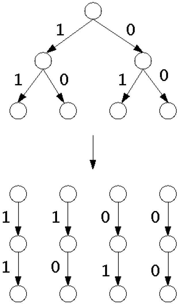 Figure 1
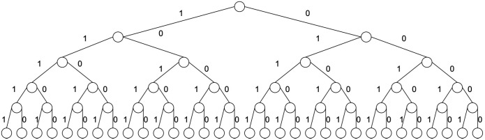 Figure 2
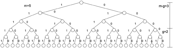 Figure 3
 Figure 4
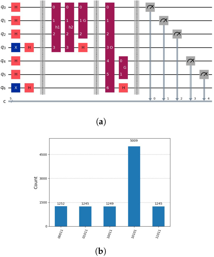 Figure 5
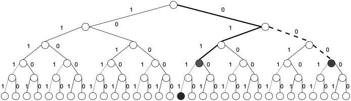 Figure 6
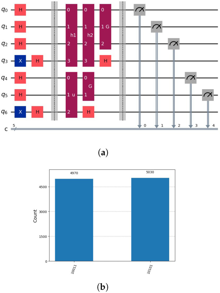 Figure 7
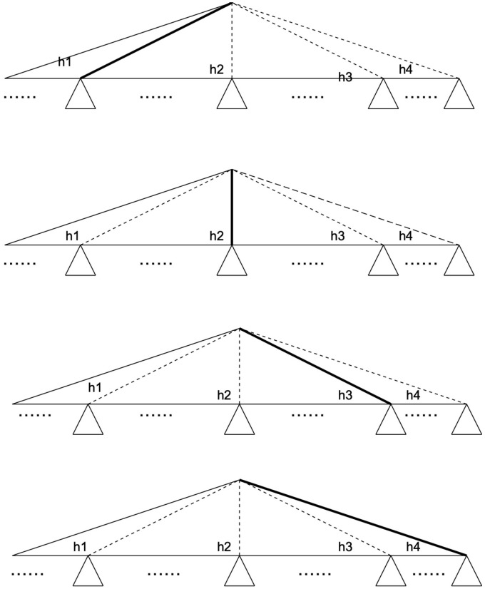 Figure 8
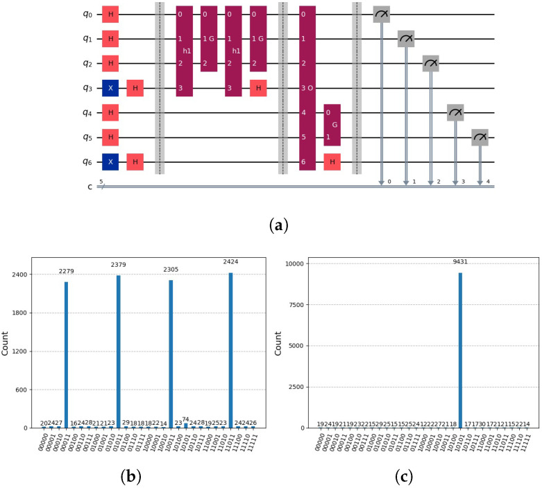 Figure 9
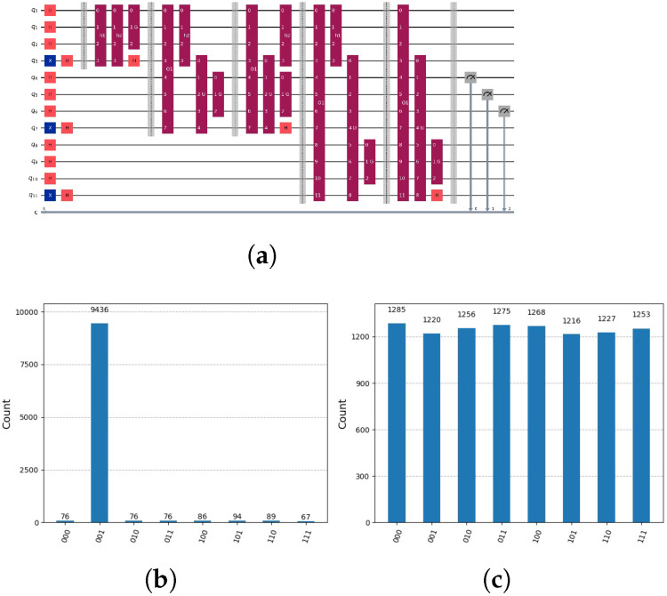 Figure 10
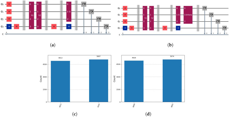 Figure 11
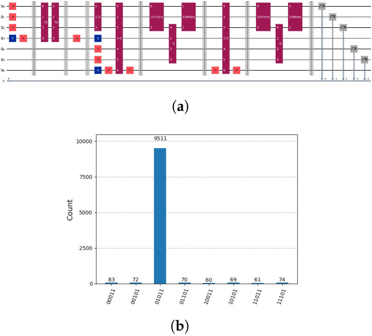 Figure 12
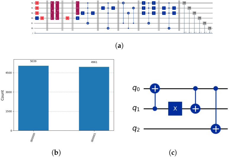 Figure 13
- —FCT, Fundação para a Ciência e a Tecnologia
Peer Reviews
No public reviews on file for this paper yet. If you reviewed it on a platform where reviews are public (OpenReview, ICLR, NeurIPS, ICML), you can paste yours below so the community can read it here.
Videos
No videos yet. Explain this paper in a talk, walkthrough, or lecture? Add one.
Taxonomy
TopicsQuantum Computing Algorithms and Architecture · Quantum Information and Cryptography · Quantum Mechanics and Applications
1. Introduction
We investigate the optimization of quantum tree search algorithms by employing a nested Grover Algorithm. We explore the implications of this approach and identify the resulting constraints. Our findings demonstrate the potential for enhanced results compared to previously developed Grover-based methods. Instead of adopting the hybrid divide-and-conquer methods that are predicated on quantum backtracking and quantum walk, as indicated in [1,2], we will proceed with the initial conception of a nested version of Grover’s nested search, as described in [3]. In a nested version of Grover search, the complete tree of partial assignments is expanded to a specific depth, and then a quantum search is conducted within the subset of partial assignments that have not yet been eliminated.
It is claimed that, for certain reasonable distributions of problems, the average complexity of the original nested version of Grover search [3] will be less than that obtained from Grover search. This claim is supported by references [1,3]. Building upon the initial concept of a nested version of Grover search, we will adopt a combinatorial approach to address the limitations inherent in the original work, as described in [3]. For simplicity, we assume that the tree is uniform and its size is known beforehand. We will demonstrate our approach on simple examples using Qiskit, see [4]. The main contributions of this paper are as follows:
- We introduce the definition of a partial candidate solution and the contented oracles.
- We analyze the constraints of the original Grover’s nested search as introduced in [3];
- We introduce the iterative approach with a quadratic speedup in comparison to the original Grover’s algorithm;
- We investigate the possibilities of dividing the original space into two disentanglement subspaces and the resulting consequences;
- We introduce the concept of performing a permutation on a subspace and the corresponding constraint.
Our approach imposes specific constraints that elucidate the concepts of partial candidate solutions within the context of quantum tree search. This work provides the foundation for quantum artificial intelligence applications, including quantum problem-solving and quantum production systems.
2. Quantum Tree Search
In this section, we outline the application of Grover’s algorithm to the tree search problem. Nodes and edges in a search tree represent states and transitions between states [5]. The initial state is the root, and from each state, either B states can be reached or it is a leaf. From a leaf no other state can be reached. b represents the branching factor of a node, indicating the number of possible choices. A leaf can either be the goal of the computation or an impasse when there are no valid transitions to a succeeding state. Each node except the root has a unique parent node, which is called the parent. Every node and its parent are connected by an edge. Each parent has b children. If and the depth of the tree is m, each of the m questions has a yes/no reply and can be represented by a bit (as shown in Figure 1). The m answers are collectively represented by a binary number of length m.
There are possible binary numbers of length m. Each binary number represents a path from the root to a leaf. For each goal, a specific binary number indicates the solution. This binary number is called a path descriptor, since it describes a path from the root of the tree to the leaf, see Figure 2 with and depth .
For a constant branching factor , each question has b possible answers. The m answers can be represented by a base-b number with m digits. In a quantum computation, we can simultaneously represent all possible path descriptors. There is one path descriptor for each leaf off the tree. Using Grover’s algorithm, we search through all possible paths and verify whether each path leads to the goal state. This type of procedure is known as a quantum tree search [6]. For possible paths, the costs are (approximately) , corresponding to the reduced branching factor .
Grover’s Algorithm
For a function
we seek to identify the value of x representing a path descriptor for which , where , the path descriptor leading to the solution. This task is equivalent to a decision problem with a binary answer: 1 indicating a successful search and 0 indicating an unsuccessful search. The instance x is the input to the problem.
Grover’s amplification algorithm implements exhaustive search in steps in an n-dimensional Hilbert space [7,8,9,10]. This algorithm is derived from the Householder reflection of the state of m qubits, where . Grover’s amplification algorithm is optimal for exhaustive search, as demonstrated by the lower bound established by [11]. One can prove that a better algorithm cannot exist [12,13]. It follows that using a quantum computer, NP-complete problems remain NP-complete. Grover’s amplification algorithm provides a quadratic speedup over classical computers, which would require n steps to solve the problem.
For k solutions and more than two qubits ( , ) the number r of iterations is the largest integer
The value of r depends on the relation of n versus k. For and we need only one rotation, and we also need only one rotation for
to find one of the k solutions. The iterative amplification algorithm requires the value of k in order to determine the number of iterations. We can determine the value of k by the quantum counting algorithm [14,15,16].
Uniform distributions are essential for Grover’s algorithm. If the distribution is non-uniform, the algorithm may not function properly or require adaptation which leads to the same complexity [3,17,18,19]. Consequently, we cannot simply mark potential solutions by assigning higher amplitude values to speed up the search. For instance, an adapted algorithm for sparse distributions where the majority of amplitudes are zero must generate a uniform distribution for the unmarked sets, with the resulting complexity [17,18,19].
In our analysis in relation to the O notation and for simplification, we will assume the approximate complexity of Grover’s algorithm as
instead of using the accurate Equation (2).
3. Nested Grover’s Search
Is it possible to integrate nested Grover’s search techniques into the quantum tree search algorithm to enhance the search process? Can the nested Grover’s search be based on heuristic functions? A heuristic function estimates the cheapest cost from a node to the goal. The local path descriptor y describes the path from the root to the node. Therefore, each node in the tree can be described by a local path descriptor. However, we cannot employ a heuristic function to generate a non-uniform distribution, as it does not confer any advantage in Grover’s search. Furthermore, we cannot compare branches represented by distinct path descriptors. This is also the reason why the min-max algorithm cannot be applied to quantum tree search in games. The reason for this is that distinct branches correspond to distinct superpositions, and these superpositions interact solely through interference.
3.1. Partial Candidate Solution
Within the context of quantum tree search, instead of employing a heuristic function , we will utilize the function , which represents a partial candidate solution, and y denotes a path from the root to the corresponding node. In contrast to the heuristic function , which can mark multiple nodes, should exclusively mark a single partial solution that includes the node indicated by the path y.
3.2. Decomposition
The idea of saving the costs is based on the inequality that represents the decomposition of the Hilbert space of dimension into subspaces and of dimension and , see Figure 3. For the value g we assume
The costs of Grover’s algorithm for the quantum tree search algorithm are
However, the costs associated with Grover’s algorithm for the quantum tree of each subspace would be significantly reduced to
(see Figure 4) with
since
because
3.3. Nested Grover’s Search and Entanglement
Following, alternatively, the idea that Grover should speed up the search on Hilbert space of dimension , a set ℵ of v partial candidate solutions
is defined that acts on g lower qubits with
on the subspace of dimension , with y being a local path descriptor. Throughout the paper, we will employ the little-endian notation, which stores the least-significant byte at the smallest address. Qubits are represented from the most significant bit (MSB) on the left to the least significant bit (LSB) on the right (little-endian), similar to binary numbers or bit-string representation on classical computers. We illustrate the fundamental concept of nested Grover search through a simple SAT example, characterized by , , and .
as indicated by the circuit in Figure 5a, with the results of measurement shown in Figure 5b. In the initial step, we determine the set ℵ using Grover’s algorithm on the subspace . In the subsequent step, we anticipate utilizing this set to expedite the search for the solution indicated by the oracle , which operates on m qubits. Grover’s amplification is applied to the subspace defined by the upper qubits. However, due to entanglement, we are unable to employ Grover’s algorithm on the upper subspace defined by upper qubits, as both subspaces and become entangled.
To comprehend the behavior we introduce concatenated oracles.
3.4. Concatenated Oracles
Concatenation is an associative operation but not a commutative operation. We use for the operation concatenation the specific symbol ‖. If we assume that x is represented by m bits with the notation
then concatenation is often simply the placement of the binary numbers next to each other,
For example, for a binary number of 10 and 11 we get
We extend the concatenation for the oracle function
Using compact notation,
and the oracle function
with
solution being
with being the upper part of the oracle function that acts on the upper qubits, describing the upper subspace of the dimension and being the lower part of the oracle function that acts on the lower qubits, describing the lower subspace of the dimension with
Note that and do not indicate partial candidate solutions; they are exact copies of the oracle function, and it can be challenging to specify them precisely. Also, u indicates the path descriptor. An example is represented in Figure 6.
In the case we constraint y values to some values with
the constraint oracle can be expressed as with
3.5. Not Entangled Subspaces
Imagine we know that acts on the upper subspace defined by lower qubits and given set ℵ of t partial candidate solutions that act on the subspace defined by upper g qubits,
If we apply both oracles and use Grover’s algorithm to each Hilbert space defined by the subspace and , the results are not entangled since both subspaces are not entangled. In the first step, we determine ℵ using Grover’s algorithm on the Hilbert space defined by the subspace . In the second step, we determine using Grover’s algorithm on the upper qubits of the upper subspace with
If we measure both subspaces, we see that each solution in the lower subspace defines a new combination of the one solution in the upper subspace . One of the combination could correspond to the global solution of the space as described by the oracle , however we do not know if this is the case.
For example in the preceding example we introduce with and
and the oracle for the upper qubits
as indicated by the circuit in Figure 7a, with the results of measurement shown in Figure 7b.
The approach can be broadly characterized as
after applying Grover’s algorithm to subspace
and the subspace
since both subspaces and are not entangled.
3.6. Entangled Subspaces
In original nested Grover’s search (see Section 3.3), after applying Grover’s algorithm to the subspace we get
both subspaces and are entangled because
Applying Grover’s algorithm to the subspace results in the creation of entanglement.
In our preceding example with (see Figure 5) after applying Grover’s algorithm to the subspace
After applying Grover’s algorithm to the subspace we get
with the state
After applying Grover’s algorithm to the subspace we get
see Figure 5b. Grover’s algorithm operates on the initial two qubits (upper qubits). It operates on two subspaces of , one for and the other for . In the subspace defined by , there is no marking. In the other subspace, there is a marking. As a result of Grover’s amplification, the first subspace exhibits a uniform distribution, while the second subspace contains a marking indicating the solution. Each of the two subspaces defined by and defined by has a probability of being measured of . In the first subspace, the uniform distribution of each state is represented by . In the second subspace, the solution is represented by , as indicated in Figure 5b. The number of partial candidate solutions, denoted as v, is inversely proportional to the probability of measuring the solution, which is represented as . How can this problem be effectively addressed? Two potential solutions to this problem are the iterative approach and the idea of the disentanglement of the two subspaces and .
4. The Iterative Approach
With the set ℵ of v partial candidate solutions
and the global oracle , we built a circuit with one possible could-be solution of the set ℵ and the global oracle. We determine in the first step one solution of one using Grover’s algorithm on the subspace , and in the second step we the global oracle acts on m qubits. Subsequently, we apply Grover’s amplification to the subspace , which is defined by the upper qubits. Figure 8 indicates an example representing the decomposed search tree for .
If a solution exists, the subspaces and are not entangled with . In this case, by measuring , we obtain the solution. This is because the number of partial candidate solutions represented in our circuit is “one,” and the probability of measuring a solution, if it exists, is We measure the state and test whether a solution is present. If it is, we terminate the process; otherwise, we select another potential solution from the set For the simple preceding SAT example with and and we get two circuits, see Figure 9.
4.1. Algorithm
Given set ℵ of v partial candidate solutions
and the global oracle .
For to v:
- 1.For the could-be solution build a circuit;
- 2.Determine the solution by Grover algorithm on the subspace ;
- 3.Verify if the solution indicated by the oracle exists;
- 4.If solution exists success, exit the loop, otherwise, continue the loop.
Since both subspaces and are not entangled, if a solution exists, it is readily apparent. We measure the state and verify whether it is a valid solution. If it is a solution, we conclude the process. Otherwise, we select another partial candidate solution from the set ℵ.
4.2. Optimal Dimension
How can we choose an optimal dimension of the two subspaces and ? The optimal dimension of the two subspaces results in the minimal costs represented by the minimum of the function
which is equivalent to
with the solution
4.3. Costs
Within the subspace , the costs associated with Grover’s algorithm are , while within the subspace , the corresponding costs remain . We need to verify the proposed solution leads to a global solution. Subsequently, we must repeat the procedure in the worst case v times, leading to the cost
with the constraint for v that the cost are below with
since . We observe that maximal possible value for v is approximately equal to the number of nodes located at one-fourth of the depth of the search tree. We can express the cost of iterative search it in O notation, given , as
5. Disentanglement of L and U
Can we disentangle the spaces and with by knowing the function ? We test the global oracle over the whole space of dimension m that defines the Hilbert space . The test should not entangle both subspaces and . We rely on the assumption that exists and can be decomposed as
Knowing , assuming the is correct and with set ℵ the task is to verify if
is true. If it is true, then we can decompose after Grover’s algorithm on the subspace
After Grover’s search on the subspace , if true,
If not true, for
and for
In the event that does not exist for any z
Since we do not know which we have to test all combinations, but we can reuse the set ℵ once computed.
After Grover’s algorithm on the subspace ,
and if u is not present we get a general superposition. We arrive at the decomposition
We have determined the correct by measuring with a probability of approximately 1 in . Subsequently, we can estimate the path descriptor using Grover’s algorithm on the subspace . The probability measurement of indicates that does not equal l and does not constitute a valid solution. However, for , it necessitates a substantial number of measurements to ascertain that the probability deviates from 1.
5.1. Example with v=2
Our previous example with
After Grover’s algorithm on the subspace we get the decomposition
with
Because of the equality we know that is correct and can estimate the path descriptor by Grover’s algorithm on the subspace .
5.2. Costs
Within the subspace , the cost associated with Grover’s algorithm is . For v combinations in the subspace , the corresponding cost is . Additionally, given , we need to determine the path descriptor by Grover’s algorithm in the subspace . The complete costs are
We can express the cost of iterative search in O notation, given that as before, with
For , the actual costs are less than the cost of the iterative algorithm with
and they are cheaper in relation to .
For , a substantial number of measurements is necessary. A practical approach would be to select , resulting in approximately faster costs
compared to the iterative approach with possible iterations.
Implementation
For the ℵ of v partial candidate solution functions that acts on g lower qubits on the subspace
we introduce a variable
and extend the upper oracle in relation to the variable
For example, for the case , . To determine a possible solution we have to measure v subspaces .
For example, in the preceding SAT example with and we introduce the variable
where corresponds to . The decomposition
is represented by the quantum circuit in Figure 10a.
6. Permutation in the Subspace L
We can map the set of solutions determined by the function of the set ℵ into in the subspace into another ordering that uses only the corresponding subset that could lead to a decomposition. For example, the superposition
is mapped by a permutation matrix P
into the decomposition , see Figure 11.
We can represent the permutation matrix P as
The operation corresponds to the mapping by permutation operator P of a register of m qubits into a register of m qubits, of which the first g qubits are , with
Since Qiskit uses little-endian notation we indicate the inverse order by a permutation matrix
into the decomposition . We can represent the permutation matrix , and due to little-endian notation we get
The operation corresponds to the mapping by permutation operator of a register of m qubits into a register of m qubits, of which the last g qubits are , with
We can apply such a permutation operator for a nested Grover’s algorithm for tree search, as indicated in Figure 12. Grover’s algorithm is applied on the qubits 2, 4 and 5.
6.1. Costs
Ignoring the costs of the permutation operator P with the preparation costs v by basis encoding in subspace , as described by [20,21,22], the costs corresponding to the Grover’s algorithm applied to qubits are
With the preparation costs using Grover’s algorithm in subspace the costs are
in O notation, given , with
6.2. Permutation Operator P
There appears to be no straightforward method to ascertain the mapping represented by P. The permutation operator P is defined by the v paths to partial could-be solutions. Due to entanglement we cannot determine the operator P using and the resulting paths. Due to entanglement we cannot determine the permutation operator P without knowing the paths that indicate which nodes indicate partial could-be solutions. Knowing the paths we can determine the permutation operator P by controlled not gates, see Figure 13a. Using the regularities, permutation operator P can be considerably compressed, see Figure 13c, leading to reduced costs.
Knowing paths defines distinct nodes of the same depth simultaneously. For instance, in the quantum search tree depicted in Figure 6, the two extended oracles would be and , with , and we would seek the solution u. This approach is appropriate for a tree search where we presume that certain nodes at a depth g signify potential solutions. Alternatively, we could implement the two extended oracles directly through a quantum circuit using concatenation.
7. Discussion
7.1. Partial Candidate Solution h(y)
Within the context of quantum tree search, instead of employing a heuristic function , we will utilize the function , which signifies a potential solution, and y represents a path from the root to the corresponding node. In contrast to the heuristic function , which can mark multiple nodes, should exclusively mark a single potential solution for the node. A set of partial candidate solutions can be identified by determining their similarity or distance to the goal state. However, how can we pinpoint a single potential solution, a single partial candidate solution? One approach to achieve this is to introduce an additional constraint that narrows the set to a single function, denoted by . Such a constraint could, for instance, specify the possible position within a subtree, thereby reducing the set to a single function. It is important to note that this approach is highly probabilistic and may occasionally yield non-existent partial candidate solutions or values exceeding one. Additionally, we have to take care that v is a constraint, as indicated by the Equation (23). In addition, further research should investigate the partial candidate solution function on examples, as indicated in the paper [5].
7.2. Generalized Quantum Tree Search
We must have prior knowledge of the depth m off the search tree. This constraint can be circumvented through iterative deepening. In an iterative deepening search, we progressively increase the search limit from one to two to three to four and continue until a goal is discovered. For each limit, a search is conducted from the root to the maximum depth of the search tree. Should the search prove unsuccessful, a new search is initiated with a deeper limit. During the iterative deepening search, states are generated multiple times [23,24]. The time complexity of an iterative deepening search is comparable to that of a search to the maximum depth [23]. A quantum iterative deepening search is equivalent to an iterative deepening search [6]. For each limit , a quantum tree search is performed from the root, where represents the maximum depth of the search tree. The potential solutions are determined through measurement.
For a non-constant branching factor, the maximal branching factor has to be used for the quantum tree search [6]. For the maximum value of , the quantum algorithm using qubit representation outperforms the classical tree search described by the effective branching factor b in the specified case
For a large number of instances with varying initial and goal states, the effective branching factor converges to the average branching factor for an uninformed tree search, as shown in [5].
Consider each branching factor as a potential local path. For a non-constant branching factor, the quantum tree search utilizes the maximal branching factor, denoted by . If, in a node , , only are required, and local paths are not utilized. To address this limitation, we augment the path descriptor by repeating the paths. This approach ultimately leads to k solutions that converge to the effective branching factor, as demonstrated in [5].
8. Conclusions
A primary outcome of the investigation is that conventional heuristic functions are unsuitable for quantum tree search due to the inability to disentangle the subspaces utilized by Grover’s algorithm. Furthermore, the theoretical concepts of the potential permutations within the subspace suggest that due to entanglement, we cannot determine the permutation operator P without knowing the paths that represent the values of the heuristic functions.
Consequently, only partial candidate solutions possess the capability to disentangle these subspaces. We assume the existence of a set of partial candidate solutions, denoted by ℵ, that can be determined, for instance, by their similarity to the goal state. We impose the constraint that within this set, only one maximal partial candidate solution, denoted by , identifies a potential solution. Each partial candidate solution of the set ℵ can be constrained to be valid only in a specific subtree. It is important to note that a partial candidate solution is not a position in the search tree itself, as its values are unknown and are determined by Grover’s algorithm and may occasionally yield non-existent partial candidate solutions or values exceeding one candidate solution.
With the existence of the partial candidate solution , the iterative approach represents a considerable speedup with the costs
We can express the cost of iterative search it in O notation, given , since as
Combinatory approach with the possible existence of the upper oracle allows us to disentangle and using
which speeds up the costs minimally.
The work suggests a novel direction based on a partial candidate solution rather than heuristic functions that are unsuitable for quantum tree search. All Qiskit (v2.2) examples are presented in a Jupyter Notebooks that can be freely downloaded at https://github.com/andrzejwichert/Nested-Quantum-Tree-Search (accessed on 16 December 2025).
The reference list from the paper itself. Each links out to its DOI / PubMed record.
- 1Montanaro A. Quantum-Walk Speedup of Backtracking Algorithms Theory Comput.20181412410.4086/toc.2018.v 014a 015 · doi ↗
- 2Rennela M. Brand S. Laarman A. Dunjko V. Hybrid divide-and-conquer approach for tree search algorithms Quantum 2023795910.22331/q-2023-03-23-959 · doi ↗
- 3Cerf N.J. Grover L.K. Williams C.P. Nested quantum search and structured problems Phys. Rev. A 20006103230310.1103/Phys Rev A.61.032303 · doi ↗
- 4Qiskit-Contributors Qiskit: An Open-Source Framework for Quantum Computing 2023 Available online: https://zenodo.org/records/8190968(accessed on 16 December 2023)
- 5Wichert A. Quantum Artificial Intelligence with Qiskit CRC Press Boca Raton, FL, USA 2024
- 6Tarrataca L. Wichert A. Quantum Iterative Deepening with an application to the Halting problem P Lo S ONE 20138 e 5730910.1371/journal.pone.005730923520465 PMC 3592860 · doi ↗ · pubmed ↗
- 7Grover L.K. A fast quantum mechanical algorithm for database search STOC ’96: Proceedings of the Twenty-Eighth Annual ACM Symposium on Theory of Computing ACM New York, NY, USA 199621221910.1145/237814.237866 · doi ↗
- 8Grover L.K. Quantum Mechanics helps in searching for a needle in a haystack Phys. Rev. Lett.19977932510.1103/Phys Rev Lett.79.325 · doi ↗